行政院國家科學委員會專題研究計畫 成果報告
高效率混合法之三相諧波潮流解析 研究成果報告(精簡版)
計 畫 類 別 : 個別型
計 畫 編 號 : NSC 99-2218-E-011-009-
執 行 期 間 : 99 年 08 月 01 日至 100 年 07 月 31 日 執 行 單 位 : 國立臺灣科技大學電機工程系
計 畫 主 持 人 : 連國龍
計畫參與人員: 碩士班研究生-兼任助理人員:黃泰迪
報 告 附 件 : 出席國際會議研究心得報告及發表論文
處 理 方 式 : 本計畫可公開查詢
中 華 民 國 100 年 09 月 24 日
1
高效率混合法之三相諧波潮流解析
黃泰迪 Tai-Di Huang1, 連國龍 Kuo-Lung Lian1
1國立台灣科技大學電機系 Department of Electrical Engineering, National Taiwan University of Science and Technology
*Corresponding Email: [email protected]
中文摘要
由 於 全 球 暖 化 與 能 源 短 缺 等 問 題,以再生能源為主的分散式發電系 統已成為當今的重要議題,為使這些 分散式系統順利與市電相接,使用了 大量的電力電子元件。另外在傳輸系 統中,電力電子彈性交流輸電系統用 來調節潮流、穩定電壓、保持系統穩 定等。然而電力電子元件之非線性特 性,會導致諧波的產生,在電力電子 元件數量激增的同時,若忽略諧波對 系統工作點之影響,將導致系統穩定 度與效能的減低。然而目前現有的電 力系統潮流解析軟體大部份只考慮基 頻時的電壓與電流,鮮少考慮諧波之 電壓與電流。因此本文以 Semlyen 教 授等人提出的時間域與頻率域混合計 算法為基礎,並改善原方法之疊代效 率且加入電力潮流之限制條件,發展 一套適用於非線性電力電子元件之電 力系統諧波潮流解析軟體。
關鍵字:時間域模型、頻率域模型、混 合法、打靶法
Abstract
Due to issues such as global warming and energy shortages, distributed generation systems empowered by renewable energy have become important topics. In order to have distributed generation units connect to the power system, it needs power electronic devices to act as interfaces. In the transmission system, power electronic based flexible ac transmission systems (FACTS) are used to adjust power flow, stabilize the voltage and keep the system steady.
Nevertheless, due to its non-linear characteristics, power electronic device produces harmonics. As the number of power electronic device increases, the effect of harmonics on the operating point cannot be ignored. Most of the current power system software, however, considers fundamental voltage and current, rarely on harmonic voltage and current. This paper proposes a new hybrid method to solve for the harmonic power flow of a power system. It essentially improves the hybrid method that Professor Semlyen has developed, to greatly reduce the number of iteration.
Such an algorithm can easily account for the harmonics produced by power electronic devices.
keyword: Time domain, frequency domain, hybrid method, shooting method
研究動機
電力供應的可靠度和服務品質,
是先進國家經濟發展重要的支撐力,
然而由於電力電子元件的大量使用,
傳統的的電力系統潮流解析技術也勢 必進行修正。在以下的四種情況本文 提出的方法能夠有所助益:
1.電力系統元件在時間域的模擬上 有其先天上的限制,為避免信號取樣 時的交疊現象,根據奈奎斯特取樣定 理,脈波寬度調變之開關控制元件其 取樣頻率至少要為所觀察最高諧波之 二倍,當開關頻率越高時,取樣之時 間步階必須越小,所需的模擬時間就 越長 。此外傳輸 線是 一種反 射之元 件,到達穩態所需之時間極長,且其 步階之選取受到行波理論之限制,步
2
階必須小於行波時間,因此會增加模 擬所需的時間[1]。
2.在尋找諧振點時使用的頻率掃描 技術,即對一個給定的電路計算出其 頻率響應,一個單位的正弦波電流以 特定的頻率範圍注入,計算出其相應 的電壓響應,計算過程按照離散的頻 率步長重複進行,以涵蓋整個頻率範 圍。如使用時間域分析法,則對每一 個掃描頻率皆需重新計算一次測試電 路直到穩態,耗時極久。
3.智能電網與再生能源為主的分散 式發電系統中,皆須使用到電力電子 轉換器設備與電網相接,但電力電子 是一種非線性元件,為了系統的穩定 度,除了考慮其產生的諧波對系統工 作點之影響,還要兼顧各轉換器間交 互作用與共振點之關係。
4.電磁暫態程序軟體,可以設定狀態 變數之初值,如果我們設定適當的初 值,則模擬結果可以跳過暫態直接進 入穩態,節省模擬的時間。
研究目的
本文主旨在提出一高效率諧波潮 流解析手法,此解析手法在收斂特性 及運算時間上皆有大幅度的改善。
文獻回顧
電力系統基頻(數位)潮流解析法 起於 1956 年由 H. W. Hale 與 J.B.
Ward [2]-[4]等人所提出,主要目的是 尋求在發電機有效功率與電壓值的規 範內,所有匯流排的電壓幅值與角度 的解[3],也就是要得到電力系統的穩 態工作點。然而當系統存在非線性元 件時,基波潮流解析無法直接求解,
必須將其隔離或以等效之線性元件代 替,在電力電子元件盛行的今天,基 頻潮流解析已無法符合實際的需要。
最 早 將 基 頻 潮 流 解 析 改 良 的 是 Heydt 與 Xia 博士,並將其改良之方法 命名為「諧波潮流解析法」[5]。此方
法雖可適用含非線性元件的電力系統,
但其並未考慮因系統不平衡或故障時 所產生的非特性諧波,只能針對非線 性元件所產生之特性諧波進行分析。
為了能同時考慮特性與非特性諧波,
有許多針對 Heydt 與 Xia 諧波潮流解析 的改良方法因此產生。改良方法可粗 略分為牛頓疊代法 [6]-[10]與逐次疊 代法 [11]-[13]兩種。牛頓疊代法是先 導出系統非線性元件的閉和行式,再 將系統的潮流問題與此閉合型式一起 以牛頓疊代算出。而逐次疊代法是使 用定點疊代法的方法將三相諧波潮流 與基頻潮流耦合,以利於將不平衡對 諧波的影響考慮進去。
但不管是 Heydt 與 Xia 之諧波潮流 解析法、牛頓疊代諧波潮流解析法或 是逐次疊代諧波潮流解析法,都是在 頻率域模擬。頻率域求解法有一先天 上的限制,就是其準確度與運算時考 慮的諧波次數極其相關,當碰到複雜 之系統時,無法準確預估該考慮的諧 波次數。若考慮的諧波次數不夠時,
碰到非線性程度高的元件時,則所得 的解與實際值誤差可達到 50%以上 [14],而如果為求精準度而考慮過多的 諧波次數時,則會大幅度地降低模擬 的效率。因此 Lian 和 Noda 提出基於 時間域諧波潮流解析的「時間域諧波 潮流解析法」[15],此法先以打靶法[16]
一種時間域的穩態演算法,使計算結 果迅速達到穩態,接著使用諧波狀態 法 [17] 在 時 間 域 計 算 實 功 率 與 虛 功 率。
但打靶法並不適用於分布參數元 件,只能運用在集總參數元件 [18]上,
故使用「時間域諧波潮流解析法」時,
當碰到分布參數元件,如傳輸線時,
需使用單一或階梯之等效 π 模型代替 分布參數模型[19]。π 模型的精準度與 階梯的數目相關,若需高精準度的解,
則階梯的數目也要提高。但階梯的電 容與電感數目[19]極其龐大時,將會導 致整個系統的模擬效率大幅降低。
3
時間域與頻率域諧波潮流解析法 都有各自的優點與缺點,若單使用一 種方法,則必將受其缺點所苦。因此 理想的方法是結合時間域與頻率域諧 波潮流解析的優點,彌補兩邊的缺點,
此觀念可見於 1995 年時 Medina 和 Semlyen 博士所提出的電力系統諧波 混合計算法[20]。此法將求解之系統分 為頻率域與時間域兩部份,將線性元 件如電容、電感、電阻等建立在頻率 域模型,而將非線性元件如可變電阻、
電容、電感或電力電子轉換器等建立 在時間域模型。這兩部分使用一諧波 電壓源 V 相接,如圖 1 所示。時間域 使用打靶法求得流入諧波電壓源 V 的 電流 IN2,而頻率域則直接使用頻率解 析法求得流入諧波電壓源 V 的電流 IN1, 最 後使 用牛 頓疊 代法 使兩 邊電 流相 等。
Medina 和 Semlyen 博士之混合法 之概念雖然簡潔清楚,但實際運算時,
因為打靶法已需一個牛頓疊代迴圈,
故實際需要兩個牛頓疊代迴圈,造成 計算效率的低弱[21]。且 Medina 和 Semlyen 博士之混合法只考慮電力系 統穩態電流與電壓而忽略了實際電力 潮 流的 限制 條件 。因 此本 論文 改良 Medina 和 Semlyen 博士之混合法,使 其能夠:
1.提升計算效率
2.符合電力系統中發電機與負載的潮 流限制條件
3.考慮電力電子元件產生之諧波對系 統工作點之影響
子系統一 頻率域
子系統二 時間域 分割處電壓
V
IN1 IN2
圖 1 研究方法
本文先實現 Semlyen 等人提出之
雙牛頓疊代迴圈法,其流程圖如圖 2 所示,先假設分割處電壓 V,頻率域 可以直接求解其分割處電流 IN1。時間 域先使用反傅立葉轉換將 V 轉換成 v(t),然後使用打靶法計算時間域的狀 態變數 x(電容電壓與電感電流),使其 在時間 0 時之 x(0),與時間在週期 T 時之 x(T)相等,再使用傅立葉轉換求得 分割處電流 IN2。比較 IN1與 IN2是否相 等,若相等則結束疊代,反之則計算 出新的分割處電壓 V,重複以上之流 程直到分割處電流相等為止。此方法 為與本文提出方法的比較基準之一。
開始
分割處電壓V(k)=[V0……VH]T
求解頻率域
反快速傅立葉轉換 (inverse Fast Fourier Transform)
在時間域設定初值x(0)(m)
在時間域求解x(T)
H(m+1)=H(m)-∆H(m) 此處 J1(m)∆H(m)=M1(m)
H=x(0) M1=x(T)-x(0) J1
(m)=∂M1/∂H
判斷是否在誤差範 圍內
使用快速傅立葉轉換 (Fast Fourier
Transform)
H(k+1)=H(k)-∆H(k) 此處 J2(k)∆H(k)=M2(k)
H=V M2=IN1+IN2
J2 (k)=∂M2/∂H
判斷是否在誤差範 圍內
結束 No
Yes
No
Yes
m=m+1
k=k+1 V
V
IN1
IN2
v(t)
圖 2
本文所提出之單牛頓疊代迴圈方 法,是將打靶法之牛頓疊代與系統整 合 之 牛 頓 疊 代 法 相 結 合 , 並 使 用 Broyden 之方法[22]建構賈可比矩陣,
其流程圖如圖 3 所示,先假設分割處
4
電壓 V 與時間域狀態變數 x,頻率域 直接求解分割處電流 IN1。時間域先使 用反傅立葉轉換計算 v(t),搭配時間 0 時之狀態變數 x(0)計算出時間域的分 割處電流 iN2(t)以及時間在週期 T 時之 狀態變數 x(T),最後使用傅立葉轉換 求出分割處電流 IN2。比較 IN1與 IN2、 x(0)與 x(T)是否相等,若相等則結束疊 代,反之則計算出新的分割處電壓 V 與時間域狀態變數 x(0),重複以上之流 程直到相等為止。
開始
分割處電壓V(k)=[V0……VH]T與x(0)(k)
求解頻率域
反快速傅立葉轉換 (inverse Fast Fourier Transform)
在時間域求解iN2(t)與x(0)
H(k+1)=H(k)-∆H(k) 此處 J(k)∆H(k)=M(k) H=[ V x(0)]T M1=[IN1+IN2 x(T)-x(0)]T
J1(k)=∂M1/∂H
判斷是否在誤差範 圍內
結束 No
Yes
k=k+1 V
V
IN1
v(t)
使用快速傅立葉轉換 (Fast Fourier
Transform)
IN2
iN2(t)
x(0)
圖 3
最後將潮流的限制條件帶入,其 流程圖如圖 4 所示,與圖 3 不同為初 始條件加入脈波寬度調變產生器中正 弦波之調變參數,且加入規劃實功率 潮流 Psch與規劃之虛功率潮流 Qsch。時 間 域 的 部 分 計 算 出 分 割 處 電 流 IN2
後,再與分割處電壓 V 計算出實功率 潮流 P 與虛功率潮流 Q。比較 IN1與 IN2、x(0)與 x(T)、P 與 Psch、Q 與 Qsch, 若皆相等則結束疊代,否則計算出新 的分割處電壓 V、時間域狀態變數 x
以及正弦波調變參數,重複整個流程 直到相等為止。
開始
分割處電壓V(k)=[V0……VH]T x(0)(k) ma theta
求解頻率域
反快速傅立葉轉換 (inverse Fast Fourier Transform)
在時間域求解iN2(t)與x(0)
H(k+1)=H(k)-∆H(k) 此處 J(k)∆H(k)=M(k) H=[ V x(0) ma theta]T M1=[IN1+IN2 x(T)-x(0) Psch-P Qsch-Q]T
J(k)=∂M1/∂H
判斷是否在誤差範 圍內
結束
No
Yes
k=k+1 V
V
IN1
v(t)
使用快速傅立葉轉換 (Fast Fourier
Transform) IN2
iN2(t)
x(0)
求解P與Q
圖 4
結果與討論
為驗正本文所提出之方法,在案 例 1,我們將比較雙牛頓疊代迴圈法及 本文提出之單牛頓疊代迴圈法,並以 PSCAD/EMTDC 驗證所得結果,求解 圖 5 之 IEEE 14 匯流排系統[23]。除電 力電子轉換器在時間域運算外,其餘 匯流排皆在頻率域運算,並以同步機 模型 [24]模擬,其資料如表 1 所示,
連接各匯流排之傳輸線為 Bergon 模 型,其幾何形狀與各項數據如圖 6 所 示。電力電子轉換器所接之變壓器為 14000/110 理想變壓器,使用正弦脈波 寬度調變控制,其正弦波振幅為 0.8、
位移角度為 3 度,其詳細電路如圖 7
5
及表 2 所示。初始疊代條件為:兩端 分割處相電壓最大值 110 伏特、時間 域之電容初始電壓與電感之初始電流 皆為 0。由表 3 可得本文提出之方法收 斂次數為雙牛頓疊代迴圈法的三分之 一、疊代所需時間也不到雙牛頓疊代 迴圈法的六分之一,在收斂效率上有 大幅度的改善。圖 8 為分割處諧波電 壓比較圖,圖 10 為分割處諧波電流比 較圖,由圖 8 及圖 9 可知本文所提出 之方法與 PSCAD/EMTDC 計算出的諧 波結果大致吻合。
converter
圖 5
Nominal power rating 100MVA Nominal voltage 14kV Nominal frequency 60Hz
R 0.005pu Lt 0.831pu Rf 0.0005pu Mdf 1pu Rs=Rt 0.02pu Mds 1pu Ld 1.2pu Mqt 0.6pu Lq 0.8pu Mfs 1pu Lf 1.2pu R0=L0 ∞ Ls 1pu
表 1
圖 6
開關頻率 540Hz Rs 25mΩ Ls 145μH Rl 4.16Ω Rf 0.15Ω Lf 0.637mH Cdc 4820μF Rdc 500Ω
表 2
Rf
Rs Ls Lf
Rl
Cdc Rdc
圖 7
6
疊代次數 疊代時間 ( pu) 雙牛頓迴
圈疊代法
6 次 6.28pu
本文提出 之方法
2 次 1pu
表 3
圖 8
圖 9
在案例 2,
我們
把潮流的限制加 入本文所提出之方法,為把焦點專注 在潮流的限制條件上,模擬如圖 10 之 4 匯流排電路,電力電子轉換器在時間 域計算,其餘匯流排在頻率域運算,並使用理想電壓源模擬,其數據如表 4 所 示 , 連 接 各 匯 流 排 之 傳 輸 線 為 Bergon 模型,其幾何形狀與各項數據
如圖 6 所示。電力電子轉換器所接之 變壓器為 14000/110 理想變壓器,實功 率與虛功率限制條件如表 4 所示,其 詳細電路如圖 7 及表 2 所示。而由表 5 可知疊代之收斂結果與規劃之電力潮 流穩合,確實達到潮流限制的目的。
PV bus1
Slack bus
PV bus2
Psch
Qsch
Psch
Psch
圖 10
Slack bus |V|=14kV 角度 0 度 PV bus1 |V|=14kV P=4416W PV bus2 |V|=14kV P=0.1822MW Converter P=6683W Q=-2391Var
表 4
規劃潮流 計算結果
PV bus1 P=4416W P=4416W
PV bus2 P=0.1822MW P=0.1822MW Converter P=6683W
Q=-2391Var
P=6698W Q=-2392Var
表 5
結論
本文以 Semlyen 教授等人提出之 雙牛頓疊代迴圈法為基礎,而提出高 效率之單牛頓疊代迴圈法,此方法的 疊代收斂次數為雙牛頓疊代迴圈法的 三分之一、疊代所需時間不到雙牛頓 疊代迴圈法的六分之一,在疊代的效 率上有大幅度的改善。此外本文提出 之方法加入了電力潮流的限制條件,
改善了原本 Semlyen 教授等人提出之 方法只考慮穩態電壓、穩態電流而忽 略潮流限制條件的缺點。
參考文獻
7 [1]EMTDCTM transient analysus for PSCADTM power system simulation uaer’s guide, pp.135.
[2] J. B. Ward and H. W. Hale, "Digital computer solution of power flow problems,"
AIEE Trans., vol. 75, pp.398-404, June 1956.
[3] B. Stott, “Review of load-flow calculation methods,”Proceedings of the IEEE, vol. 62, no.
7, pp.916-929, July 1974.
[4] J. Grainger and W. D. Stevenson, Power Systems Analysis, International edition, 1994.
[5] D. Xia and G. T. Heydt,“Harmonic Power Flow Studies Part I - Formulation and Solution,”IEEE Transactions on Power Apparatus and Systems, Vol. PAS-101, No. 6, pp.1257 – 1265, June 1982.
[6] B. C. Smith and J. Arrillaga, “Power flow constrained harmonic analysis in ac-dc power systems,”IEEE Transaction on Power Systems, vol. 14, no. 4, pp. 1251-1261, Oct. 1999.
[7] B. C. Smith, N. R. Watson, A. R. Wood, and J. Arrillaga, “A Newton solution for the harmonic phasor analysis of AC/DC converters,”
IEEE Transactions on Power Delivery, Vol. 11, No. 2, pp. 965 – 971, April
1996.
[8] G. N. Bathurst, B. C. Smith, N. R. Watson, and J. Arrillaga,“Modelling of HVDC transmission systems in the harmonic domain,”IEEE Transactions on Power Delivery, Vol. 14, No. 3, pp. 1075 – 1080, July
1999.
[9] C. N. Bathurst, B. C. Smith, N. R. Watson, and J. Arrillaga, “A modular approach to the solution of the three-phase harmonic power-flow,”IEEE Transactions on Power Delivery, Vol. 15, No. 3, pp. 984 – 989,
July 2000.
[10] Q. N. Dinh, J. Arrillaga, and B. C. Smith,
“Steady-state model of direct connected generator-HVDC converter units in the harmonic domain,”IEE Proceedings-Generation, Transmission and Distribution, Vol.
145, No. 5, pp. 559 – 565, Sept. 1998.
[11] M. Valacarcel and J. Mayordomo,
“Harmonic power flow for unbalanced systems,”
IEEE Transactions on Power Delivery, Vol. 8, No. 4, pp. 2052-2059, Oct. 1993.
[12] W. Xu, J. R. Marti, and H. W. Dommel, “A multiphase harmonic load flow solution technique,” IEEE Transactions on Power Delivery, Vol. 6, No. 1, pp. 174-182, Feb. 1991.
[13] J. G. Mayordomo, L. F. Beites, R. Asensi, F.
Orzaez, M. Izzeddine and L. Zabala,“A contribution for modeling controlled and uncontrolled AC/DC converters in harmonic power flows,”IEEE Transactions on Power Delivery, Vol. 13, No. 4, Oct. 1998, pp. 1501 - 1508
[14] P. W. Lehn and K. L. Lian, “Frequency
coupling matrix of a voltage source converter derived from piecewise linear differential equations,” IEEE Transactions on Power Delivery, Vol. 22, No. 3, pp. 1603-1612,July 2007.
[15] K. L. Lian, and T. Noda, “Development of an electromagnetic transient analysis program for power systems (Part 2): development of a fundamental algorithm for steady-state calculation,” 日 本 電 力 中 央 研 究 所 報 告 書 (H07004), 2008.
[16] T. J. Aprille, T. N. Trick,“Steady-state analysis of nonlinear circuits with periodic inputs, ”Proceedings of the IEEE, Vol. 60, No. 1, pp.108 – 114, Jan. 1972.
[17] P. W. Lehn and K. L. Lian, “Frequency coupling matrix of a voltage source converter derived from piecewise linear differential equations,” IEEE Transactions on Power Delivery, Vol. 22, No. 3, pp. 1603-1612,July 2007.
[18] K. S. Kundert, "Steady state methods for simulating analog circuits," Ph. D. dissertation, University of California, Berkeley, 1989.
[19] C. Christopoulos, The Transmission-Line Modeling (TLM) Method in Electromagnetics, Morgan &Claypool publishers, 2006.
[20] A. Semlyen and A. Medina, “Computation of the periodic steady state in systems with nonlinear components using a hybrid time and frequency domain methodology,” IEEE Transactions on Power Systems,
[21] K. L. Lian and T. Noda, "A Three-Phase Harmonic Power Flow Algorithm Based on A Hybrid Approach", International Conference on Power Systems Transients, Kyoto Japan, June 2-6, 2009.
[22] R. L. Burden and J. D. Faires, Numerical Analysis, 7th Edition, 2001.
[23] Richard D. Christie, Power Systems Test Case Archive, Dept. of Electrical Engineering, University of Washington, Seattle, WA, http://www.ee.washington.edu/research/pstca/
[24]A. Semlyen, J.F. Eggleston, J. Arrillaga,
“Admittance Matrix Model of a Synchronous Machine for Harmonics Analysis”, IEEE Transactions on power Systems, Vol. 2, No. 4, November 1987, pp. 833-840.
國科會補助專題研究計畫項下出席國際學術會議心得報告
日期: 100 年 9 月 25
日
一、參加會議經過
此次會議有三個目的:(a)與各國研究學者交流並交換意見、分享成果及 學習其他創新解析手法。(b)訓練學生上台用英語報告、回答。(c)將在本 計劃所研發的演算法用於最佳電力潮流計算(optimal power flow),並在國 際會議發表並聽取專家意見。
二、與會心得
此次會議收獲甚多,其中演算手法與專家交換意見,可總結於以下兩點 1.Neural network based model 可能無法用於 account for reactive power dispatch
2. Transmission line load effects also need to be considered.
三、攜回資料名稱及內容 帶回大會全論文摘要集(1 CD) 四、其他
研討論文如附件 計畫編
號
NSC
99-2218 - E - 011 - 009 -計畫名
稱
高效率混合法之三相諧波潮流解析
出國人
員姓名 連國龍
服務機 構及職
稱
台灣科技大學
會議時 間
100 年 7 月 4 日至 100 年 7 月 7 日
會議地 點
Bali, Indonesia
會議名 稱
The 12th International Conference on Quality in Research 發表論
文題目
The Lagrange Optimal Power Flow with Generator Capability
Curves as Constraints
The Lagr ange Optimal Power Flow (LOPF) with Gener ator Capability Cur ves as Constr aints
Mat Syai’ina,b, Kuo Lung Liana , Adi Soepr ijantob
a Electrical Engineering Department, National Taiwan of University Science and Technology , Taipei, Taiwan E-mail : [email protected]; [email protected]
b Electrical Engineering Department, Sepuluh Nopember Institute of Technology , Surabaya, Indonesia E-mail : [email protected]; [email protected]
ABSTRACT
This paper presents how the generator capability curve (GCC) of a generator can be included in a Lagrange optimal power flow (LOPF). Normally, the constraints for a generator in an optimal power flow (OPF) are defined as rectangular constraints (Pmin-Pmax, Qmin-Qmax). However, such constraints may overestimate the cost of the generation. Therefore, it is the objective of this paper to see how much cost can be reduced if a GCC can be included in an OPF. A neural network (NN) model will be derived to model a GCC. The main advantage of an NN model is that a GCC can be obtained easily without deriving complicated equations. A 16-bus system with 3 generators will be presented in this paper to show that a total saving of 759.31 $/ hr can be achieved if the GCCs for the three generators are included in an LOPF.
Keywor ds
Lagrange Optimal Power Flow, Generator Capability Curve, Neural Network
1. INTRODUCTION
The objective of an optimal power flow (OPF) is to minimize the total fuel cost of the generating units, usually having quadratic cost characteristics, which is subjected to active, reactive power, bus voltage, and line flow limits.
To minimize quadratic cost function, the Lagrange multiplier method is one of well-known methods that have been applied in OPF. To establish the necessary conditions for an extreme value of the objective function, it adds the constraint function to the objective function after the constraint functions have been multiplied by an undetermined multiplier [1].
Recently, the issue of global warming and energy crisis becomes an important topic. Many researchs aims to find alternative energy sources, to overcome the problem of energy crisis. In addition, improving efficiency of the existing apparatus is also very important to reduce cost operation. In this paper, we put more emphasis on energy efficiency, especially optimal power flow (OPF). Many OPF methods have been developed based either on conventional methods or artificial intelligence methods [2-12], but almost all those methods used rectanguler constraint to limit the generator output. However, in actual operations, a generator’s limitations are definied by the generator capability curve (GCC). Hence, it is the purpose of this paper to investigate how the results would differ for an optimal power flow based on GCC constraint and that based on the rectanguler constraint [13-15].
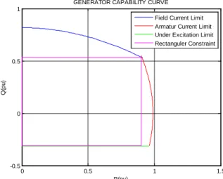
Fig.1 shows the GCC, which is constructed based on field currents, armature currents and under excitation limits [16]. As noted in the figure, an optimal power flow based on the rectanguler constraint may lead to higher operation cost as some of the utilization area (area betwen outside rectanguler and inside curve) are not included. On the other hand, using GCCs[16] as constraints in OPF [13,15] require complicated equations. Neural Network (NN) consequently is used in this paper to model the GCC as it does not require the use of complicated equations [17]. A GCC, constructed using a NN can be applied not only as a constraint in the Lagrange optimal power flow (LOPF) but also in other OPF methods[17]. In this paper, we will show that operating cost will be reduced if GCC is used as a constraint in the LOPF.
2. METHODOLOGY
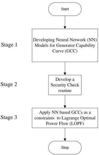
The proposed algorithm consists of three stages, which are as follows.
1. Develop NN models for GCCs.
2. Develop a security check routine.
3. Apply the NN-based GCCs as constraints to the Lagrange Optimal Power Flow (LOPF).
Fig. 2 shows the overall flow chart of the methodology. The following subsections will explain the implementation steps in each stage.
Figure 1: Comparison Rectanguler Constraint and Generator Capability Curve (GCC) Constraint
0 0.5 1 1.5
-0.5 0 0.5 1
P(pu)
Q(pu)
GENERATOR CAPABILITY CURVE
Field Current Limit Armatur Current Limit Under Excitation Limit Rectanguler Constraint
Start
Developing Neural Network (NN) Models for Generator Capability
Curve (GCC)
Develop a Security Check
routine
Apply NN based GCCs as a constraints to Lagrange Optimal
Power Flow (LOPF)
Stop
Stage 1
Stage 2
Stage 3
Figure 2: Stage of design LOPF with GCC constraint based on NN
2.1 Develop Neur al Networ k (NN) Models for Gener ator Capability Cur ves.
The proposed NN model for a generator capability curve is very straightforward as it only has one input, one output and one hidden layer, as shown in Fig. 3. The number of neuron in hidden layer is constructed automaticaly by using constructive backpropagation method [19].
1
2
3
4
n Hidden Layer In
put
Out put
Figure 3: NN model for generator capability curve
P (MW)
Q(Mvar)
R
Ɵ
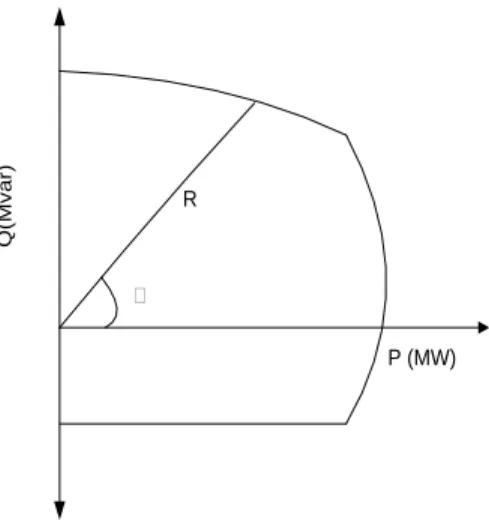
Figure 4: The illustration of the input and output
The input data used in the training process are the sampling point data along the GCC line curves provided by generator manufactures’ data sheet. Since the GCC is spanned over a plane, it has two directions x and y directions. This makes the computation extremely difficult. To simplify the computation process, we convert all the (P, Q) pairs into the polar coordinates, (R,θ) pairs as shown in Fig. 4. Once θ is chosen, we only need to compute the length, R. Therefore, θ will be our input for the training process and R will be the output of the NN. The proper weighting and number of neurons in the hidden layer are then determined to construct the complete GCC curves. The reconstructed GCC curves are set as the constraints in the optimal power flow.
2.2 Develop a Secur ity Check Routine.
The converged P,Q values obtained in the load flow need to be checked against these GCC constraints. The checking process can be accomplished in the following three steps:
1. The converged P, Q values are first converted into polar pairs (R, θ).
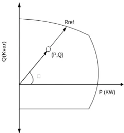
2. The value of θ can be used to determine the distance from the origin to the GCC curve, Rref, as shown in Fig. 5.
3. The generator security can be checked by comparing the value of R and Rref. If R ≤ Rref, the converged P, Q are within the safety limits; otherwise, they are set to the values converted from (Rref, θ).
P (KW)
Q(Kvar)
Rref
Ɵ (P,Q)
Figure 5: Relationship between P,Q, θ, R and Rref
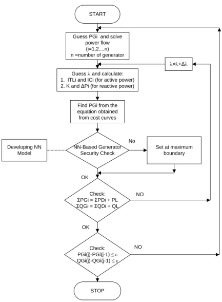
2.3 Apply NN-based GCCs as constr aints to Lagr ange Optimal Power Flow (LOPF).
The steps in applying NN-based GCCs constraints to Lagrange Optimal Power Flow (LOPF) are as follows (see Fig.
6):
1. Generate initial conditions for the real power of the generation unit i, PGi, and run power flow.
2. Generate initial value for the Lagrange multiplier λ and calculate incremental transmission loss associated with generation unit i, ITLi and the incremental cost of generation unit i, ICi (for active power). Moreover, one also needs to calculate the positive factor K and the partial derivatives of the real power losses with respect to the reactive power, ΔP (for reactive power). Note that the expressions for ITLi, ICi, K and ΔP can be found in reference [18].
3. Find PGi from the equation obtained from the characteristic of cost curve.
4. Check PGi and QGi using security check routine (Sub section 2.2) to see if the position of PGi and QGi are within the GCC.
5. Check the equality constraints:
∑ 𝑃𝐺𝑖=∑ 𝑃𝐷𝑖+ 𝑃𝐿 (1)
∑ 𝑄𝐺𝑖=∑ 𝑄𝐷𝑖+ 𝑄𝐿 (2)
If the equality constraints are not satisfied, change the value of λ and go to step 2; otherwise, go to step 6 6. Check the error tolerance (e)
|𝑃𝐺𝑖𝑗− 𝑃𝐺𝑖𝑗−1| ≤ 𝑒 (3)
|𝑄𝐺𝑖𝑗− 𝑄𝐺𝑖𝑗−1| ≤ 𝑒, (4) where j is the iteration number
If (3) and (4) are not satisfied, go to step 1 and re-initialize the value of PGi
If (3) and (4) are satisfied, the solution has reached, and the iteration process terminates.
START
NN-Based Generator Security Check
Check:
ΣPGi = ΣPDi + PL ΣQGi = ΣQDi + QL
STOP
No
OK Developing NN
Model
Set at maximum boundary Guess PGi and solve
power flow (i=1,2....n) n =number of generator
Guess λ and calculate:
1. ITLi and ICi (for active power) 2. K and ΔPi (for reactive power)
Find PGi from the equation obtained from cost curves
λ=λ+Δλ
Check:
PGi(j)-PGi(j-1) ≤ ε QGi(j)-QGi(j-1) ≤ ε
OK
NO
NO
Figure 6: Flowchart of the proposed LOPF
3. RESULT AND ANALYSIS
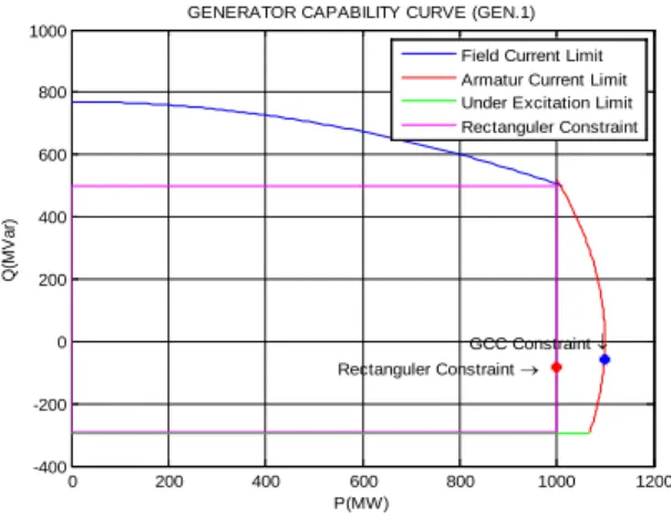
A 16-bus system with 3 generators was studied. Two scenarios were compared. One is based on the LOPF with rectangular curves as the generator constraints. The other is based on the LOPF with GCC as the generator constraints. Table I shows the converged simulations results for both scenarios. As can be noted, 759.31 $/ hr of saving can be achieved by the LOPF with GCC as the generator constraints.
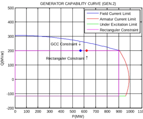
Data from TABLE I can be plotted in Figs. 7 – 9. Fig. 7 shows the operating cost saving occurs because the generator 1 which has characteristics of low-cost generation is operated at maximum capability curve. Figs. 8 and 9 show the operations for generator 2 and 3, respectively.
Table 1: Cost generation and converged powers.
Figure 8: Comparison between the rectangular constraints and GCC constraints for geneartor 1
0 200 400 600 800 1000 1200
-400 -200 0 200 400 600 800 1000
Rectanguler Constraint → GCC Constraint ↓
P(MW)
Q(MVar)
GENERATOR CAPABILITY CURVE (GEN.1)
Field Current Limit Armatur Current Limit Under Excitation Limit Rectanguler Constraint
LPSO-OPFWITHRECTANGULAR CONSTRAINT LPSO-OPFWITHGCC CONSTRAINT No of
Generator P(MW) Q(MVar) COST($/hr) No of
Generator P(MW) Q(MVar) COST($/hr) 1
2 3
1000.00 622.60 320.66
-82.21 200.00 43.75
17144.04 8130.95 9165.84
1 2 3
1100.0 568.58 276.12
-58.75 200.00 47.83
16700.00 8236.96 8744.57
Total Cost 34440.83 Total Cost 33681.52
Figure 9: Comparison between rectangular constraints and GCC constraints for geneartor 2
Figure 10: Comparison between the rectangular constraints and GCC constraints at geneartor 3
4. CONCLUSSION
In this paper, we have shown how an LOPF can include GCCs as constraints. The challenge of including the GCC constraints in the LOPF is the complex equations describing these curves. As has been delineated in the paper, an NN was proposed and constructed for modeling a GCC. Such a model can be easily incorporated into an LOPF.
Finally, the simulation study presented in this paper shows that reduction of cost can be achieved if a GCC, rather than the conventional rectangular constraint is used in an OPF.
REFERENCES
[1] Allen J. Wood and B.F., Wollenberg,. “Power Generation Operation and Control” by John Wiley & Sons, Editor. 1996. p.
29-90., 514-559.
[2] B. Venkatesh, M.K. George, and H. B. Gooi, "Fuzzy OPF incorporating UPFC," IEE Proceedings-Generation, Transmission and Distribution, 2004. 151(5): p. 625-629.
[3] H. Mori and T. Horiguchi, "A genetic algorithm based approach to economic load dispatching," ANNPS '93.
[4] W. Yurong, L. Fangxing, and W. Qiulan, "Reactive power planning based on fuzzy clustering and multivariate linear regression," IEEE Power and Energy Society General Meeting, 2010.
0 100 200 300 400 500 600 700 800 900 1000 1100 -200
-100 0 100 200 300 400 500
Rectanguler Constraint ↑ GCC Constraint ↓
P(MW)
Q(MVar)
GENERATOR CAPABILITY CURVE (GEN.2)
Field Current Limit Armatur Current Limit Under Excitation Limit Rectanguler Constraint
0 100 200 300 400 500 600 700
-200 -100 0 100 200 300 400 500
Rectanguler Constraint ↑ GCC Constraint ↓
P(MW)
Q(MVar)
GENERATOR CAPABILITY CURVE (GEN.3)
Field Current Limit Armatur Current Limit Under Excitation Limit Rectanguler Constraint
[5] M. A. Abido, "Multiobjective particle swarm optimization for optimal power flow problem," MEPCON 2008.
[6] L. dos Santos Coelho and V.C. Mariani. "Economic dispatch optimization using hybrid chaotic particle swarm optimizer,"
ISIC 2007.
[7] J. Park, Y. Jeong, J. Shin and K. Y. Lee, "An Improved Particle Swarm Optimization for Nonconvex Economic Dispatch Problems," IEEE Trans. on Power Systems, 2010. 25(1): p. 156-166.
[8] W. Liu., L. Min, and W. Xianjia. “An improved particle swarm optimization algorithm for optimal power flow”. IPEMC '09.
[9] R.R.B. Aquino, et al. "Recurrent neural networks solving a real large scale mid-term scheduling for power plants," in IJCNN 2010.
[10] C. A. Roa-Sepulveda and B. J. Pavez-Lazo, "A solution to the optimal power flow using simulated annealing," IEEE Porto.
2001.
[11] K. K. Swarnkar, S. Wadhwani, and A. K. Wadhwani. "Optimal Power Flow of large distribution system solution for Combined Economic Emission Dispatch Problem using Partical Swarm Optimization," ICPS '09.
[12] S. Panta and S. Premrudeepreechacharn, "Economic dispatch for power generation using artificial neural network," ICPE '07.
[13] P. E. Onate Yumbla, J.M. Ramirez, and C.A. Coello Coello, "Optimal Power Flow Subject to Security Constraints Solved With a Particle Swarm Optimizer," IEEE Transactions on Power Systems, 2008. 23 (1): p. 33-40.
[14] G. B. Sheble, "Real-Time Economic Dispatch and Reserve Allocation Using Merit Order Loading and Linear Programming Rules," IEEE Power Engineering Review, , 1989. 9(11): p. 37-37.
[15] G. Zwe-Lee, "Particle swarm optimization to solving the economic dispatch considering the generator constraints," IEEE Trans. on Power Systems, 2003. 18(3): p. 1187-1195.
[16] P. E. Sutherland, "Generator capability study for offshore oil platform," Industrial & Commercial Power Systems Technical Conference 2009.
[17] M. Syai'in, A. Soeprijanto,, and T. Hiyama, "Generator Capability Curve Constraint for PSO Based Optimal Power Flow,"
International Journal of Electrical and Electronics Engineering, 2010. 4(6): p. 371-376.
[18] J. F. Dopazo, O. A. Klitin, G. W. Stagg and M. Watson, "An optimization technique for real and reactive power allocation,"
Proceedings of the IEEE, 1967. 55(11): p. 1877-1885.
[19] N. Gunaseeli and N. Karthikeyan, "A Constructive Approach of Modified Standard Backpropagation Algorithm with Optimum Initialization for Feedforward Neural Networks," Computational Intelligence and Multimedia Applications, 2007
國科會補助專題研究計畫項下出席國際學術會議心得報告
日期: 100 年 9 月 25
日
一、參加會議經過
濟州 2011 年微型電網研討會的目的是透過此會議讓各國研究
微型電網之專家能對當前微型電網研究,關鍵技術,經濟和政策及未來 的研究應該解決的問題作相互交流。前六個研討會分別於 2005 年在美國 伯克利分校,2006 年在加拿大蒙特朗布朗,2007 年在日本名古屋,2008 年希臘 Kythnos 島,2009 年美國聖地亞哥及 2010 年加拿大溫哥華。
此次榮幸受到大會邀請參加並以 poster 方式報導成果。此次會議有兩個目 的:(a)與各國研究學者交流並交換意見、分享成果及學習其他創新解析 手法。(b)將在本計劃所研發的演算法用於最佳電力潮流計算(optimal power flow),並在國際會議發表並聽取專家意見。
二、與會心得
此次為初次參加此會議,所學甚多。北美地區的微型電網建置佔全世界 44%,暫居世界第一。值得台灣學習借鏡。以下的專題是目前一些研究機 構或電力公司所研究的議題,值得參考研究
-Electric vehicle integration and smart charging -AMI and demand response
計畫編 號
NSC
99-2218 - E - 011 - 009 -計畫名
稱
高效率混合法之三相諧波潮流解析
出國人
員姓名 連國龍
服務機 構及職
稱
台灣科技大學
會議時 間
100 年 5 月 26 日至
100 年 5 月 27 日
會議地 點
Jeju Island
會議名 稱
The Jeju 2011 Symposium on Microgrids 發表論
文題目
The Lagrange Optimal Power Flow (LOPF) with Generator
Capability Curves as Constraints
-Renewable energy integration -Automatic fault location
-Advanced recloser technologies -Automatic reconfiguration
-Remote management of distribution automation equipment
另外,林法正 招集人也以應邀出席並發以講講方式對本國的智慧型電網 之投資及建設作詳細的說明,也描述對本國在微型電網及智慧電網中的 各中長期主要計畫。
此次會議也安排到濟州島的微型電網的展示中心,了解其能源管理中心 之運作。
三、攜回資料名稱及內容 帶回大會全論文摘要集(1 CD) 四、其他
研討 poster 如附件
The Lagrange Optimal Power Flow (LOPF) with Generator Capability Curves as Constraints
Mat Syai’ina, Kuo Lung Lianb , Adi Soeprijantoc
a,bElectrical Engineering Department, National Taiwan of University Science and Technology , Taipei, Taiwan E-mail : [email protected]; [email protected]
cElectrical Engineering Department, Sepuluh Nopember Institute of Technology , Surabaya, Indonesia E-mail : [email protected]
Abstract-Normally, the constraints for a generator in an optimal power flow (OPF) are defined as rectangular constraints (Pmin-Pmax, Qmin-Qmax).
However, such constraints may overestimate the cost of the generation. Therefore, it is the objective of this paper to see how much cost can be reduced if a GCC can be included in an OPF. A neural network (NN) model is derived to model a GCC. The main advantage of an NN model is that a GCC can be obtained easily without deriving complicated equations. A 16-bus system with 3 generators will be presented in this paper to show that a total saving of 759.31 $/ hr can be achieved if the GCCs for the three generators are included in an LOPF.
II. METHODOLOGY I. INTRODUCTION
Many OPF methods have been developed based either on conventional methods or artificial intelligence methods. However, almost all those methods used rectanguler constraint to limit the generator output. In actual operations, a generator’s limitations are definied by the generator capability curve (GCC). Hence, it is the purpose of this paper to investigate how the results would differ for an optimal power flow based on GCC constraint and that based on the rectanguler constraint .
III. RESULT
LPSO-OPF WITH RECTANGULAR CONSTRAINT LPSO-OPF WITH GCC CONSTRAINT
No of
Generator P(MW) Q(MVar) COST($/HR) No of
Generator P(MW) Q(MVar) COST($/HR) 1
2 3
1000.00 622.60 320.66
-82.21 200.00 43.75
17144.04 8130.95 9165.84
1 2 3
1100.05 68.58 276.12
-58.75 200.00 47.83
16700.00 8236.96 8744.57
Total Cost 34440.83 Total Cost 33681.52
RECTANGULAR CONSTRAINT GCC CONSTRAINT
No of
Bus V(pu) Delta (pu) P(MW) Q(MVAR) No of Bus
V(p u)
Delta
(pu) P(MW) Q(MVAR
)
1 1 0 643.1484 -107.631 1 1 0 642.656 -146.761
2
1.001 0.134154 800 200
2 1.0
3 0.122525 800 244.6312 3
0.98 -0.01051 500 56.70188
3 0.9
8 -0.00883 500 40.15485
0 200 400 600 800 1000 1200
-400 -200 0 200 400 600 800 1000
Rectanguler Constraint → GCC Constraint ↓
P(MW)
Q(MVar)
GENERATOR CAPABILITY CURVE (GEN.1)
Field Current Limit Armatur Current Limit Under Excitation Limit Rectanguler Constraint
0 200 400 600 800 1000 1200
-200 -100 0 100 200 300 400
↑ Rectanguler Constraint GCC Constraint →
P(MW)
Q(MVar)
GENERATOR CAPABILITY CURVE (GEN.2)
Field Current Limit Armatur Current Limit Under Excitation Limit Rectanguler Constraint
IV. CONCLUSION
The challenge of including the GCC constraints in the LOPF is the complex equations describing these curves. As has been delineated in the paper, an NN was proposed and constructed for modeling a GCC. Such a model can be easily incorporated into an LOPF. Finally, the simulation study shows that reduction of cost can be achieved if a GCC, rather than the conventional rectangular constraint is used in an OPF.
Fig.2 Comparison Rectangular Constraint and RGCC Constraint at geneartor 1
Fig.3 Comparison Rectangular Constraint and RGCC Constraint at geneartor 2 in case of voltage control
TABLE I
Additional Power Supply and Cost of Generation
TABLE II
Voltage and Frequency
0 200 400 600 800 1000
-600 -400 -200 0 200 400 600
Active Power(MWatt)
Reactive Power(MVar)
PAITON CAPABILITY CURVE
GCC data sheet GCC based on NN
To develop a NN model for a GCC. The data used in the training process of the NN are the sample points along a GCC provided by the generator manufacture’s data sheet. NN model consists of one input, one output and one hidden layer. To obtain the weighting coefficients of the NN, we first convert all the (P, Q) pairs into the polar forms, (R,θ). Then, we set θ as the input and R as the output. The weighting coefficients can consequenly be obtained via constructive backpropagation method. Hence, one can easily restore a GCC for a given values ofθ.
國科會補助計畫衍生研發成果推廣資料表
日期:2011/09/20
國科會補助計畫
計畫名稱: 高效率混合法之三相諧波潮流解析 計畫主持人: 連國龍
計畫編號: 99-2218-E-011-009- 學門領域: 電力系統
無研發成果推廣資料
99 年度專題研究計畫研究成果彙整表
計畫主持人:連國龍 計畫編號:99-2218-E-011-009- 計畫名稱:高效率混合法之三相諧波潮流解析
量化
成果項目 實際已達成
數(被接受 或已發表)
預期總達成 數(含實際已
達成數)
本計畫實 際貢獻百
分比
單位
備 註 ( 質 化 說 明:如 數 個 計 畫 共 同 成 果、成 果 列 為 該 期 刊 之 封 面 故 事 ...
等)
期刊論文 0 0 100%
研究報告/技術報告 0 0 100%
研討會論文 0 0 100%
論文著作 篇
專書 0 0 100%
申請中件數 0 0 100%
專利 已獲得件數 0 0 100% 件
件數 0 0 100% 件
技術移轉
權利金 0 0 100% 千元
碩士生 1 1 100%
此 碩 士 生 由 此 計 畫支付其薪支,其 負 責 項 目 為 撰 寫 程 式 及 部 份 精 簡 報告。
博士生 1 1 100%
此 博 士 生 由 其 它 計 畫 支 付 其 薪 支,但部份研發成 果亦用於此計畫。
博士後研究員 0 0 100%
國內
參與計畫人力
(本國籍)
專任助理 0 0 100%
人次
期刊論文 1 1 100%
本 計 劃 之 部 分 成 果 及 創 新 解 析 手 法已投稿於 IEEE Transactions on Circuits and Systems I:
Regular papers。
且已於近期接受。
研究報告/技術報告 0 0 100%
研討會論文 1 1 100%
篇
本 計 劃 之 部 分 創 新 解 析 手 法 延 伸 已 於 The 12th International Conference on Quality in Research 發表。
國外
論文著作
專書 0 0 100% 章/本
申請中件數 0 0 100%
專利 已獲得件數 0 0 100% 件
件數 0 0 100% 件
技術移轉
權利金 0 0 100% 千元
碩士生 0 0 100%
博士生 0 0 100%
博士後研究員 0 0 100%
參與計畫人力
(外國籍)
專任助理 0 0 100%
人次
其他成果
(
無法以量化表達之成 果如辦理學術活動、獲 得獎項、重要國際合 作、研究成果國際影響 力及其他協助產業技 術發展之具體效益事 項等,請以文字敘述填 列。)無
成果項目 量化 名稱或內容性質簡述
測驗工具(含質性與量性) 0
課程/模組 0
電腦及網路系統或工具 0
教材 0
舉辦之活動/競賽 0
研討會/工作坊 0
電子報、網站 0
科 教 處 計 畫 加 填 項
目 計畫成果推廣之參與(閱聽)人數 0
國科會補助專題研究計畫成果報告自評表
請就研究內容與原計畫相符程度、達成預期目標情況、研究成果之學術或應用價 值(簡要敘述成果所代表之意義、價值、影響或進一步發展之可能性) 、是否適 合在學術期刊發表或申請專利、主要發現或其他有關價值等,作一綜合評估。
1. 請就研究內容與原計畫相符程度、達成預期目標情況作一綜合評估
■達成目標
□未達成目標(請說明,以 100 字為限)
□實驗失敗
□因故實驗中斷
□其他原因 說明:
2. 研究成果在學術期刊發表或申請專利等情形:
論文:■已發表 □未發表之文稿 □撰寫中 □無 專利:□已獲得 □申請中 ■無
技轉:□已技轉 □洽談中 ■無 其他:(以 100 字為限)
3. 請依學術成就、技術創新、社會影響等方面,評估研究成果之學術或應用價 值(簡要敘述成果所代表之意義、價值、影響或進一步發展之可能性)(以 500 字為限)
本計劃延伸現有諧波解析手法之一的混合法,減少牛頓迭代迴圈,使其更有效率。此法可用 於 microgrid 或 smart grid 系統上,以解析大量電力電子元件所產生諧波對系統的影響。
本計劃之部分成果及創新解析手法已投稿於 IEEE Transactions on Circuits and Systems I: Regular papers。 且已於近期接受。本計劃之部分創新解析手法延伸已於 The 12th International Conference on Quality in Research 發表。