具有位移及角度量測功能之全像式原子力顯微鏡之設計與開發

國立臺灣大學工學院機械工程學研究所 博士論文

Department of Mechanical Engineering College of Engineering

National Taiwan University Ph.D. Dissertation

具有位移及角度量測功能之全像式原子力顯微鏡 之設計與開發

Design and Development of HOE-based Atomic Force Microscope with Translational and Angular Measurements

莊博景 Bo-Jing Juang

指導教授：黃光裕 博士

Advisor: Kuang-Yuh Huang, Dr.-Ing

中華民國 104 年 6 月

June 2015

誌謝

能夠完成這篇論文，我要特別感謝指導老師黃光裕教授。老師對學術的專業與 堅持，以及對學生的付出，都令人敬佩；在研究上的獨到眼光，宏觀且具遠見，

指引學生一步一步前進，讓學生在研究及生活處事的態度上受益良多。同時感謝 中研院張嘉升老師、黃英碩老師所提供的研究環境，讓學生可以在其中不斷學習，

並獲得啟發。另外感謝邱雅萍老師、廖洺漢老師以及楊志文博士在百忙之中撥空 為我口試，為學生的研究提供寶貴的意見。

此外，胡恩德博士、廖先順博士，感謝你們的研究奠定了深厚基礎，才讓我有 機會攀著前輩的肩膀看的更遠；感謝信廷、國贊、天仁、秉純、律妏，因為有你 們一起開發，才讓這研究主題越來越豐富；中研院的同事：敬修、偉珉、仲翔、

仁峰、宣富、揚文，因為有你們的陪伴及幫忙才讓我能順利完成論文，尤其是丁 丁，謝謝你在實驗上不斷地幫我破關升級；也感謝台大實驗室每一位成員的支持 與協助，總是讓我能夠遠端解決事情。另外，我還想感謝長期關心我論文進度的 余岳仲老師、李世炳老師、胡蔓莉師母、王裕鑫先生、吳喜成先生、韋僑、莉穎、

雅綾、賢真、敏麒、哲誠、嘉良、誼伶、王秀鑾女士、陳洪玉花女士…；以及這 些年來默默支援我的好友：惠暄、一如、宜瑩、惠禎；以及林呈應先生所帶領的 精工室團隊。當然我也沒忘了解散已久的不三不四團員：淇文、亮兆、千桂，機 電光同學和中原群俠的所有伙伴。要感謝的人真的太多無法一一列出，謝謝所有 關心我的朋友。

我也想將此論文獻給我的雙親莊化導先生和莊劉美珍女士，以及家人（閔仁、

登化、岱樺、智琄、俊愷），因為有您們的栽培，才讓我有機會一直繼續學業；親

愛的亮君、子誼還有二寶，感謝妳們在我埋首研究之際，給予我最大的支持與包 容；也感謝岳父母提供天龍國住宿卷以及在生活上的教誨。最後，希望本論文對 相關研究者能提供一點點助益。

中文摘要

原子力顯微鏡廣泛應用在工程及科學領域，尤其在奈米量測的重要性與日俱增。

本論文發展具有位移與角度量測功能的全像式原子力顯微鏡，並開發可在空氣及 水溶液中掃描的機制。相較以光槓桿原理為光學頭的原子力顯微鏡體積較大，且 需要花費較多時間做光路的調整。全像式光學元件具有體積小而緊緻與高靈敏度 的優點，以全像式讀取頭作為原子力顯微鏡光學頭，除了方便控制外更可縮短光 路調整時間；經由透鏡的組合可達到所需的掃描範圍，以提升原子力顯微鏡的設 計彈性與性能。

透過理論推導與軟體分析，本論文選用適合原子力顯微鏡架構的準直鏡與物鏡，

並以理論及實驗方式說明全像式讀取頭具有量測位移及角度變化的能力；透過熱 雜訊頻譜的分析，驗證全像式讀取頭的高靈敏度；也利用熱雜訊頻譜及聚焦誤差 訊號的關係，推導出非接觸式量測微懸臂彈性係數的方法。

經實驗證明，本論文所架構之全像式原子力顯微鏡在空氣中及水溶液中掃描石 墨樣品皆達到單層石墨台階解析度，利用循軌誤差訊號做角度的回饋亦可達到奈 米等級解析度，掃瞄結果說明全像式原子力顯微鏡的高解析度及穩定性。此外，

利用讀取頭的光學特性，全像式系統也適用於非接觸式光學輪廓儀的應用，藉由 不同樣品的掃描也驗證該模式的可行性。

關鍵字：原子力顯微鏡、全像式光學元件、位移量測、角度量測

Abstract

Recent years have seen increased attention being given to atomic force microscopy (AFM) in nano-scale measurement. In this dissertation, a holographic optical element (HOE) based AFM is designed and developed for operation in air and water. Unlike the bulk size and cumbersome procedures of laser beam deflection method, holographic pickup head has the advantages of easy control and simpler optical adjustment. The features of compact configuration, small size, and high sensitivity let HOE enhance the performance of AFM.

Through theoretical analysis and software simulation, the translational S-curve between the light spot on photodiode and reflective plane displacement is deduced.

According to the simulation results, the relevance of light spot shape, translational displacement, bending angle, and torsional angle are revealed. The detection functions of translational and angular displacements of the cantilever are demonstrated. The experiment of thermal noise spectrum verifies the stable performance and high sensitivity of holographic pickup head. The spring constant calibration of a micro cantilever is also derivative by thermal fluctuation method.

AFM images of graphite display the single layer step (0.34 nm) in both air and water.

The nanometer scale resolution by track error signal is also divided, thus verifying the resolution and stability of HOE-based AFM system. The images of non-contact optical profiler mode for microcircuit and tuberose epidermis tissue exemplify the feasibility and applicability of HOE-based profiler system in micron scale.

Keywords：Atomic force microscopy, Holographic optical element, Translational measurement, Angular measurement

Contents

誌謝.. ...i

中文摘要 ... ii

Abstract ... iii

Contents ...iv

List of Figures ... vii

List of Tables ...xi

List of Symbols ... xii

Chapter 1 Introduction ... 1

1.1 Motivation ... 1

1.2 Literature Survey ... 2

1.2.1 Atomic force microscopy ... 2

1.2.2 AFM in liquid ... 6

1.2.3 Optical pickup head in AFM ... 9

1.3 Thesis Organization ... 12

Chapter 2 Theoretical Analysis and Simulation ... 13

2.1 Introduction of HOE ... 13

2.2 Theoretical Analysis of HOE ... 19

2.2.1 Ray-tracking of diffracted beam ... 19

2.2.2 Spot size and depth of focus ... 25

2.2.3 Optical analysis in liquid ... 27

2.3 Simulation of HOE ... 29

2.3.1 Focus error signal and translational deflection ... 29

2.3.2 Tracking error signal and torsional signal ... 31

2.3.3 Translational S-curve in air and water ... 34

2.4 Cantilever Dynamics ... 36

2.4.1 Cantilever dimensional effect ... 36

2.4.2 Cantilever dynamics in air and water ... 38

Chapter 3 Performance of Holographic Pickup Head ... 42

3.1 Properties of Holographic Pickup Head ... 42

3.1.1 Depth of focus and linear region ... 42

3.1.2 Tracking error signaland torsional signal ... 45

3.1.3 Effect of water layer ... 48

3.2 Thermal Fluctuation Spectrum ... 51

3.3 Spring Constant Calibration ... 53

3.3.1 Thermal fluctuation method ... 53

3.3.2 Experimental setup and calibration results ... 54

3.4 Cantilever Motion Measurement ... 60

3.4.1 Translational measurement ... 60

3.4.2 Angular measurement ... 62

Chapter 4 HOE-based AFM ... 65

4.1 Configuration of HOE-based AFM ... 65

4.1.1 Scanning platform ... 67

4.1.2 AFM probe holder ... 68

4.1.3 Holographic pickup head ... 70

4.1.4 Signal acquisition system ... 72

4.2 Performance Verification of HOE-based AFM ... 74

4.2.1 Dynamic and measurement performance ... 74

4.2.3 Measurement by tracking errorsignal ... 81

4.3 HOE-based Profiler and Implementation ... 83

Chapter 5 Conclusion ... 87

Reference ... 89

Appendix ... 95

List of Figures

Figure 1.1 World’s first AFM experimental setup ... 3

Figure 1.2 Scheme of cantilever deflection detection ... 4

Figure 1.3 Comparison between resonant frequencies in air and liquid ... 7

Figure 1.4 Comparison of different stimulated cantilever responses in water ... 8

Figure 1.5 Configuration of AFM with a compact disk pickup head ... 9

Figure 1.6 Configuration of DVD-based AFM ... 10

Figure 2.1 Configuration of astigmatic pickup head and holographic pickup head ... 14

Figure 2.2 Schematic view of HOE unit ... 15

Figure 2.3 HOE unit versus astigmatic pickup head ... 15

Figure 2.4 Patterns and SEM image of HOE six-segment photodiode ... 16

Figure 2.5 Configuration and translational S-curve of holographic pickup head ... 18

Figure 2.6 Schematic ray-tacking of holographic pickup head ... 19

Figure 2.7 Refraction of skew ray ... 21

Figure 2.8 Transmission grating diffraction ... 22

Figure 2.9 Diffraction of incident beam ... 22

Figure 2.10 Projected spot on photodiode coordinate ... 24

Figure 2.11 Focusing path of laser beam ... 26

Figure 2.12 Effect of numerical aperture on lateral resolution ... 27

Figure 2.13 Focusing path of laser beam in liquid ... 28

Figure 2.14 Definition of deflections ... 29

Figure 2.15 Optical simulation model ... 30

Figure 2.16 Simulated spots for translational displacement Sz from -20 to 20 μm ... 30

Figure 2.17 Focus error signal U and translational displacement Sz ... 31

Figure 2.18 Simulated spots on photodiode for different bending angles ... 32

Figure 2.19 Relationship between tracking error signal UTES and bending angle θy ... 32

Figure 2.20 Simulated spots on photodiode for different torsional angles ... 33

Figure 2.21 Relationship between torsional signal UTR and torsional angle ... 34

Figure 2.22 Optical simulation model in water ... 34

Figure 2.23 Simulated translational S-curve in air and water ... 35

Figure 2.24 Geometric dimensions of rectangular cantilever... 36

Figure 2.25 Analytical amplitude spectrum of PPP-NCH in air and water ... 40

Figure 2.26 Analytical amplitude spectrum of PPP-CONT in air and water ... 41 

Figure 3.1 Configuration of translational S-curve measurement setup ... 42

Figure 3.2 Transltional S-curve of different objective lens ... 44

Figure 3.3 Simulation and experimental results of focus error signal UFES ... 45

Figure 3.4 Setup for measuring tracking error signal UTES and torsional signal UTR ... 46

Figure 3.5 Simulation and experimental results of tracking error signal UTES ... 47

Figure 3. 6 Simulation and experimental results of torsional signal UTR ... 48

Figure 3.7 Configuration of water thickness effect experimental setup ... 49

Figure 3.8 Measured translational S-curves for different water thicknesses ... 49

Figure 3.9 Influence of water layer on maximum S-curve range Up-p and linear region 50 Figure 3.10 Thermal fluctuation spectrum of PPP-CONT cantilever ... 52

Figure 3.11 Thermal spectra by focus error signal UFES and tracking error signal UTES 52 Figure 3.12 Configuration of spring constant experimental setup ... 55

Figure 3.13 Construction of spring constant experimental setup ... 56

Figure 3.14 SEM image of AFM probe CSC38/Cr-Au ... 56

Figure 3.15 Translational S-curve of CSC38 cantilevers ... 57

Figure 3.16 Thermal fluctuation spectrum of CSC38 ... 58

Figure 3.17 Force curve of CSC38 cantilevers on graphite substrate ... 59

Figure 3.18 Configuration of translational measurement setup ... 61

Figure 3.19 Measured vertical displacement versus translational signal ... 61

Figure 3.20 Configuration of angular measurement setup ... 62

Figure 3.21 Measurement results of bending angle versus angular signal ... 63

Figure 3.22 Implementation of AFM probe with Lorentz force actuation ... 64

Figure 3.23 Frequency spectrum by electro-magnetic excitation in air ... 64

Figure 4.1 Configuration of HOE-based AFM ... 66

Figure 4.2 HOE-based AFM ... 67

Figure 4.3 Construction and photograph of scanning platform ... 67

Figure 4.4 Construction and photograph of AFM probe holder. ... 68

Figure 4.5 Spectra of stimulated cantilever in water ... 69

Figure 4.6 Spectra of stimulated cantilever in air and water ... 70

Figure 4.7 Construction and photograph of holographic pickup head ... 71

Figure 4.8 Configuration of signal acquisition system ... 72

Figure 4.9 Photograph of signal acquisition system ... 73

Figure 4.10 Bending excitation spectrum of PPP-NCH probe in air ... 75

Figure 4.11 Force curve on TGQ1 grating ... 75

Figure 4.12 Topographic image and cross-sectional profile of sample TGQ1 in air... 76

Figure 4.13 Cantilever properties on HOPG sample in air ... 77

Figure 4.14 Topographic image and cross-sectional profile of HOPG sample in air ... 78

Figure 4.15 Construction of probe holder with water drop ... 79

Figure 4.16 Cantilever properties on HOPG sample in water ... 80 Figure 4.17 Topographic image and cross-sectional profile of HOPG sample in water 80

Figure 4.19 AFM image and cross-sectional profile of HOPG sample with UTES ... 82

Figure 4.20 HOE-based profiler ... 84

Figure 4.21 Profiler images of calibration grating TGZ3 ... 85

Figure 4.22 SEM and profiler images of HOE photodiode ... 86

Figure 4.23 Optical and profiler images of tuberose epidermis tissue ... 86

List of Tables

Table 2.1 Parameters of theoretical analysis………39

Table 3.1 Specification of lens ... 43

Table 3.2 Linear regions and deduced linear ratios of different objective lens ... 44

Table 3.3 Deduced data of translational S-curve for different water thicknesses ... 50

Table 3.4 Spring constant calibration results of AFM and HOE ... 60

List of Symbols

Symbol Description Unit

D distance from the object point to incidence point mm

D0 diameter of the entrance pupil mm

d distance between collimator and objective lens mm

dg groove spacing μm

D1 first segment photodiode ---

D2 second segment photodiode ---

D3 third segment photodiode ---

D4 fourth segment photodiode ---

D5 fifth segment photodiode ---

D6 sixth segment photodiode ---

E Young’s modulus GPa

F0 amplitude of oscillatory force N

f focal length mm

HA transmission grating A ---

HB transmission grating B ---

HC transmission grating C ---

h thickness of cantilever μm

hair the length form airy focal point to glass surface mm

hglass thickness of cover glass mm

hliquid thickness of liquid mm

hwater thickness of water mm

I moment of inertia μm⁴

K incidence unit vector of X direction ---

K' refraction unit vector of X direction ---

k spring constant N/m

kB Boltzmann’s constant m ∙ kg/ s ∙ K

k’ incidence normal vector of X direction ---

L incidence unit vector of Y direction ---

L’ refraction unit vector of Y direction ---

l length of cantilever μm

l' incidence normal vector of Y direction ---

M incidence unit vector of Z direction ---

M’ refraction unit vector of Z direction ---

m diffraction order ---

mg mass of cantilever g

m' incidence normal vector of Z direction ---

N

refraction normal vector ---

NA numerical aperture ---

n refractive index of media before refracting --- n' refractive index of media after refracting ---

nair refractive index of air ---

nglass refractive index of glass ---

nliquid refractive index of liquid ---

Q quality factor ---

Sz translational deflection along Z-axis μm

T absolute temperature K

t time sec

UD1 output voltage of D1 V

UD2 output voltage of D2 V

UD3 output voltage of D3 V

UD4 output voltage of D4 V

UD5 output voltage of D5 V

UD1 output voltage of D6 V

UFES focus error signal V

Up-p peak to peak voltage of S-curve V

UTES tracking error signal V

UTR torsional signal V

W0 Beam waist mm

w width of cantilever μm

X0 X coordinate at the plane of refraction mm

Y0 Y coordinate at the plane of refraction mm

Z0 Z coordinate at the plane of refraction mm

ZR Rayleigh length mm

z vertical movement of cantilever mm

λ wavelength μm

α one axis of direction cosines coordinate ---

αi incidence coordinate of α-axis ---

αm diffraction coordinate of α-axis at m order ---

β another axis of direction cosines coordinate ---

βi incidence coordinate of β-axis ---

βm diffraction coordinate of β-axis at m order ---

γ damping coefficient ---

μ mass per unit length kg/m

ρ density kg/m³

ρair density of air kg/m³

ρc density of cantilever kg/m³

ρwater density of water kg/m³

ρf fluid density kg/m³

η viscosity Pas

ηair viscosity of air Pas

ηwater viscosity of water Pas

θair refraction angle of air degree

θi incidence angle before grating degree

θglass refraction angle of glass degree

θliquid refraction angle of liquid degree

θx angular displacement around X-axis degree

θy angular displacement around Y-axis degree

φm diffraction angle of m order ---

ω0 free resonant frequency kHz

ωr resonant frequency in fluid kHz

ωvac resonant frequency in vacuum kHz

 angle between the direction of grating and α-axis degree

Chapter 1 Introduction

1.1 Motivation

For the last three decades, the research in scanning probe microscopy (SPM), and atomic force microscopy (AFM) have gathered greater importance. AFM approaches the development of nano-scale observation in many fields. With the development of high-speed AFM, more and more scientists use this instrument to improve their research.

Most AFM heads adopt the optical beam deflection principle to detect the deflection of the cantilever tip and to control the interaction force between the tip and the specimen surface. Some AFM heads use astigmatic pickup heads which can simplify the adjustment operation. With the development of digital video disc (DVD) system, it is not only to develop short-wavelength blue-ray disc, but also to launch smaller holographic pickup heads. Holographic pickup head includes a holographic optical element (HOE) which can replace some optical components in an astigmatic pickup head. HOE is also very compact and with a stable and precise sensing performance. Furthermore, HOE can effectively miniaturize the entire optical detection module and simplifies its adjustment operation.

HOE can also separately detect the translational motion and the angular motion of the cantilever with high sensitivity. The angle detection function can provides AFM with another operation mode.

For surface topography measurement, optical profiler is another technique. During the process, optical profiler does not touch the surface so that it cannot be damaged by surface wear. The holographic pickup head can provide a tiny focus spot size and raises the lateral resolution through focusing. By using the holographic pickup head to measure the topography of sample surface, HOE can apply both in optical profiler and AFM application.

The dissertation proposes a new developed holographic pickup head for the AFM application. Owing to the advantages of small laser spot, high bandwidth, compact structure and high sensing performance, HOE makes the surface measurement system more flexible and diversified.

1.2 Literature Survey 1.2.1 Atomic force microscopy

In order to know more information of surface science, scientists developed some instruments for measuring. The first stylus profiler had been invented by Schmalz[1] in 1929. Then, Young et al.[2], demonstrated a non-contact stylus profiler to measure the surface microtopography. Unlike optical microscope, stylus profiler can detect more fine structure with a sharpened probe. Stylus profiler does not depend on electron beam to produce an image which like electron microscope, but can achieve nano-scale resolution.

In 1982, Binnig and Rohrer.[3] invented the scanning tunneling microscope (STM) with a metal tip at constant tunnel current. This invention opened the door of atomic scale measurement and manipulation. Some years later in 1986, Binnig et al.[4] developed the atomic force microscope (AFM), which combined the principles of the STM and the stylus profiler. Figure 1.1 expresses the first AFM experimental setup. In this setup, the STM and AFM piezoelectric drives are facing each other, and sandwiching the diamond tip that is glued to the cantilever. The cantilever is fixed to a modulating piezo element which is used to drive the cantilever beam at its resonant frequency. A feedback loop is used to keep the force acting on the stylus at a constant level. Viton spacers are used to damp the mechanical vibrations. AFM images are obtained by measurement the force on the tip created by the proximity to the surface of the sample. In this method, the samples

are not limited to metal materials, AFM opened the possibility to precisely detect any nonconductive surface.

Figure 1.1 World’s first AFM experimental setup [4]

Most AFM relies the beam deflection method for cantilever deflection detection[5].

Figure 1.2 shows the scheme of cantilever deflection detection which consists of a light source, a cantilever with a reflective surface and a photoelectronic sensor. Due to the atomic interaction force between the probe and the specimen surface, the cantilever deforms and lets the projected light beam reflect back to the photoelectronic sensor.

According to the cantilever’s deformation, the reflective light spot on the photoelectronic sensor varies its shape and position. Through enlarging the distance between the cantilever and the sensor, the motion of the reflective light spot can be magnified to derive a high sensing resolution. According to the nature of the tip motion, AFM imaging modes normally include three modes: contact mode, tapping mode and non-contact mode.

Figure 1.2 Scheme of cantilever deflection detection [5]

Contact AFM is the oldest AFM operation mode in which the tip is brought into direct contact with the surface. In contact mode, the repulsive force, between the tip and the sample, is set by pushing the cantilever against the sample surface with Z-scanner. The repulsive force is small (about 10^-6 to 10^-10 N) and sensitive to distance. The normal force with the lateral motion during the scanning brings out the friction. Therefore, the excessive force will damage or move the sample, especially for the soft material in liquid.

It is very important to select the appropriate force to get the preferred resolution. The contact mode AFM is easier to get atomic resolution.

Non-contact mode was presented by Martin et al.[6]. An attractive force, which is the long-range force between the tip and the sample at a small distance (1-10 nm), is used to measure the surface. The amplitude and the phase of the cantilever vibration are monitored by a Z-axis feedback loop system which is used to control the distance of the tip and the sample. Therefore, a high speed Z-scanner is required to track the change the tip-sample distance. Compared with contact mode AFM, non-contact mode AFM uses the smaller force (generally about 10^-12 N) for scanning, the soft samples can be imaged

There are two major operation modes in dynamic-mode AFM, which are amplitude modulation mode and frequency modulation mode. Amplitude modulation AFM (AM-AFM) is usually known as tapping mode that was first introduced by Zhong et al. in 1993[7]. In this mode, the cantilever oscillates at its resonant frequency with oscillation of 20 to 100 nm larger than those in the non-contact mode. When the tip approaches to the sample surface, the interaction of forces (van der Waals forces, intermolecular forces, electrostatic forces, etc.) causes the decrease of the cantilever oscillation amplitude. The root mean square (RMS) value of the deflection detector is used to control the height between the tip and the sample. The set point value of the modified oscillation amplitude is used to adjust at a constant value as the tip scanning. Imaging the force of the intermittent contacts of the tip with the sample surface, a tapping mode image is produced.

Owning to the influence of the high frequency cantilever knocking, the tip may be defaced when scanning on hard surface, while a soft sample, the sample may be damaged.

In order to strengthen performance, the AFM is capable of several related modes with different detections. Besides the typical contact/non-contact mode and tapping mode, several modes are available for measuring various physical properties. For example, in the contact mode, the lateral force mode[8] and the force modulation mode[9] are derived.

Lateral force mode measures the deflection (or twisting) of the cantilever in the horizontal direction. That is dependent on the frictional force acting on tip. The results of lateral force AFM image the variations of surface friction, and enhance by edge deflection of surface feature. Force modulation is used a mechanical oscillation to the tip during the scanning. By measuring the amplitude of oscillation and the offsets of the phase signal to map the differences in surface stiffness or elasticity.

Phase mode imaging is by mapping the phase lag of the cantilever oscillation relative

to the signal sent to the piezo driving the cantilever[10]. In this mode, variations of surface properties such as elasticity, adhesion and friction are given. Two-pass technique, like magnetic force microscopy (MFM) is used to measure the magnetic domain by the magnetized tip that coated with ferromagnetic film. Electrostatic force microscopy (EFM) measures the electric field gradient and distribution on the sample surface through applying a bias between the tip and the sample. Furthermore, there are other resonant modes like the scanning capacitance microscopy (SCM) and the scanning kelvin microscopy (SKM), etc.

1.2.2 AFM in liquid

For the biological applications, AFM is adaptive to various environments not only in air, vacuum, but also in liquid. However, the liquid viscosity significantly dampens the dynamic properties such as the resonant frequency and the quality factor (Q-factor). The resonant frequency drops owing to the large effective mass of the cantilever in liquid. The high damping reduces the Q-factor of the system and lowers the force sensitivity.

Sulchek et al. presented the transfer function of a freely vibrating ZnO cantilever in air and water[11]. Figure 1.3 illustrates the frequency spectra in air and liquid. In water, the resonant frequency is strongly amped. The frequency shifts from 56 to 35 kHz and the Q-factor reduces from 110 to 3.

Figure 1.3 Comparison between resonant frequencies in air and liquid[11]

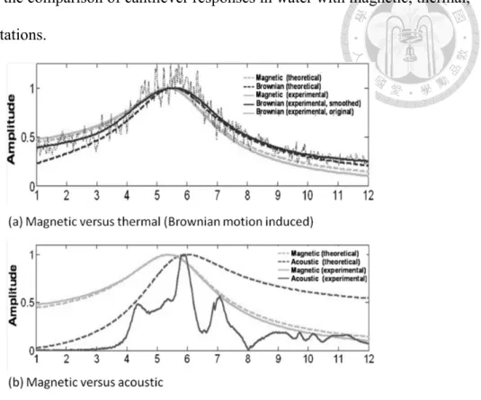
In addition, the excitation spectrum in liquid is usually not so pure than in air. There are usually many peaks in the cantilever frequency response spectrum that are not related directly to the cantilever resonance. It was suggested that the peaks were due to fluid cell resonance or mechanical resonance (piezo, chip, chip holder, etc.). The research of excitation modes were developed to get pure cantilever resonance in liquid. In AFM, different types of excitation can be grouped into three different categories: dither piezo/acoustic, direct forcing, and sample excitation[12]. Dither piezo/acoustic is simple operating, but there are some mechanical elements between the piezo plate and the cantilever. The piezo expansion and contraction cause the base of the cantilever to move up and down with an amount. In response, the cantilever is displaced relative to the chip by an amount. Comparison of the direct forcing case, a force acts directly on the cantilever, there is no relative motion. The direct forcing methods include: piezoelectric cantilever[13], magnetic method[14], electrostatic excitation[15], photothermal method[16], self-actuating[17], and quartz tuning forks[18]. Xu and Raman compared the magnetic, acoustic, and thermal excitations of the cantilever in liquid[19]. The results showed that the thermal excitation and magnetic excitation are subtle. Many artificial resonance peaks arise in the frequency spectrum of the experimental acoustic excitation.

Figure 1.4 shows the comparison of cantilever responses in water with magnetic, thermal, and acoustic excitations.

Figure 1.4 Comparison of different stimulated cantilever responses in water [19]

The AFM images of biological molecules must be intuitive, real-time, and dynamic.

Ando et al. presented the development of the high-speed AFM that enables to directly visualize the structures and dynamic of biomolecules at a short time[20]. There are three key factors for realizing high-speed Bio-AFM[21]: (i) high feedback bandwidth based on fast devices, (ii) active damping to suppress the mechanical vibrations of scanner, and (iii) make high-speed imaging compatible with low-invasive imaging. Therefore, some techniques such as small cantilever[22], fast amplitude detector[23], high-speed scanner[24], active damping technique, and fast phase detector[25], were developed for high-speed AFM.

1.2.3 Optical pickup head in AFM

In 1999, Quercioli et al. presented a study that used a compact disk (CD) pickup as the cantilever position sensor in an AFM[26]. Both the optical lever detection and the astigmatic pickup head are combined to monitor the vertical displacement of the cantilever in an AFM. It is equipped with an optical microscope for accurate the selected scanning region, sample visual inspection, and the light spot of the cantilever position alignment. The width of the linear region of the curve is about 4 μm with a slope of 0.86 V/μm. The RMS noise is ±2.5 nm. The cross-sectional profiles of AFM image can achieve nanometer scale, but not reached atomic scale. Figure 1.5 shows the configuration of AFM with a compact disk pickup head.

Figure 1.5 Configuration of AFM with a compact disk pickup head [26]

With the development of the digital versatile disc (DVD), the short laser wavelength

and bigger numerical aperture of objective lens make the pickup head has the ability to measure higher optical storage density. In 2005, Hwu et al. proceeded to apply the CD/DVD pickup head in an AFM[27-29]. Figure 1.6 illustrates the configuration of AFM with modified DVD optical head. The contact, non-contact, and tapping modes are demonstrated in the astigmatic pickup head system. The single atomic steps of graphite can be resolved by the DVD-based AFM. Further, an astigmatic detection system (ADS) is used to achieve real-time measurements of linear displacement and 2D tile angle with high sensitivity. Utilizing the ADS, the thermal vibrations of the AFM cantilever is also detected. The advantages of the small light spot and high bandwidth of the DVD pickup head let the ADS can be used to characterize the static and dynamic mechanical response of AFM cantilever and open new applications in many technological fields.

Figure 1.6 Configuration of DVD-based AFM [28]

Liao et al. used the DVD pickup head in AFM for the liquid environment[30]. The optimized ADS was demonstrated to achieve good contrast and good spatial resolution of cancer cells in water with optical profiler mode. The experimental results indicated that

atomic steps on graphite and DNA modules on mica are imaged in water.

Recently, based on an astigmatic detection system, a high-speed atomic force microscope was developed[31]. HS-AFM enables visualizing dynamic behavior of biological molecules at a temporal time (less than 1 second). DVD pickup head with high bandwidth of 80 MHz is sufficient for the scanner at high scam rate. A high-speed scanner was fabricated for fast scanning. A small cantilever with resonant frequency of 5.5 MHz is adopted at scan rate up to 200 line/s (average speed of 1.5 mm/s). AFM topographic images of grating sample showed the high quality without significant degradation.

1.3 Thesis Organization

The dissertation is structured as follow:

The first chapter gives an introduction for the research background and the motivation.

The developments of atomic force microscope and optical pickup head system are also referred in this chapter.

The second chapter is about the theoretical analysis and the software simulation. The optical principle and derivation of holographic optical system are analyzed by ray-tracking method. Through the simulation of the optical path, the relationship between the light spot and reflection plane is discussed.

Based on the analysis, the performances of holographic optical system are verified in Chapter 3. The resolution of holographic optical system with different object lens is examined, the thermal fluctuation spectrum with the high sensitivity of holographic pickup head is described. Using the thermal fluctuation method, the spring constant calibration process is presented. Besides, the translational and angular measurements are also provided in this chapter.

In Chapter 4, HOE-based atomic force microscope is developed. Through the test on Si-made rectangular grating and the graphite specimen, the feasibility and the behavior of the HOE-based AFM system are demonstrated. The results of experimental test for atomic force microscope and optical profiler are presented. Finally, a conclusion of this dissertation is drawn in Chapter 5.

Chapter 2 Theoretical Analysis and Simulation

In this chapter, the theoretical analysis and the software simulation are discussed. The optical principle and derivation of holographic optical system are analyzed by ray-tracking method. Through the simulation of the optical path, the relationship between the light spot and reflection plane is discussed. Utilizing the theoretical analysis, the relationship between the light spot and the photodiode is realized. According to the simulation results, the relevance of light spot, translational displacement, bending angle, and torsional angle are revealed.

2.1 Introduction of HOE

In 1988, Kimura et al.[32] used a holographic optical element for a CD player.

Compared with the astigmatic pickup head, which consisting of a laser-diode source, grating, polarizing beam splitter, collimator, objective lens, concave lens and a four-quadrant photodiode. HOE instead of the grating, the beam splitter and the concave lens and combined with the laser diode and photodiode. Figure 2.1 shows the configuration of an astigmatic pickup head and a holographic pickup head. The specs of pickup heads are minimized for more compact configuration. In addition, HOE is packaged in a thin-shell plastic housing instead of a conventional metal housing. These improvements have not only reduced the size and weight of optical pickup head, but also improved the stability. Because of the consolidated advantages of compact configuration, small size, and lightweight, HOE can be a beneficial key component for precision measurement.

Figure 2.1 Configuration of astigmatic pickup head and holographic pickup head [32]

An HOE unit consists of a hologram grating, a laser diode chip, and a photodiode chip.

The hologram grating can be fabricated through some lithographic process. A light beam diffracted by the semicircular portion is responsible for laser focusing function, and the two quadrant gratings on the rear side are used for position tracking function. The laser chip and the photodiode chip are mounted in a hermetically sealed package. In order to simultaneously satisfy the CD/DVD applications, an HOE unit contains with two laser sources with wavelengths of 650 and 780 nm. Figure2.2 illustrates the schematic view of HOE unit. The desired first-order diffracted beam is obtained through the grating. The higher-order diffracted beams are close to the first-order beam, but their intensities are very weak. For simplifying the optical path, the schematic diagram only shows the first-order diffracted beam.

Figure 2.2 Schematic view of HOE unit [33]

Figure 2.3(a) shows the photograph of the HOE unit (GH6D307B5A, SHARP) which is integrated with a laser diode, a hologram, and a six-segment photodiode. It is 10 mm long × 8 mm wide × 3 mm thick. The HOE unit is with a high speed response optical integrated circuit (OPIC) for CD/DVD applications. An OPIC consists of a light detecting element and signal-processing circuit integrated into a single chip.[34] Compared with a commercial astigmatic pickup head, HOE has a noticeably smaller size that is shown in Figure 2.3(b).

Figure 2.3 HOE unit versus astigmatic pickup head

The hologram includes various grating pitches, which are designed with the saw-tooth shape. The pattern has three regions in which the directions of the grating are different.

The three transmission gratings HA, HB and HC diffract the reflected laser beam focused on the six-segments photodiode D1, D2, D3, D4, D5, and D6. The semicircular portion diffracts the reflected laser beam to focus on the line dividing segments D3 and D4.

Segments D2 and D5 are auxiliary segments for accurate focus error detection. The diffracted sub-beam of the reflected tracking beam is converged on segments D1 and D6.

Figure 2.4(a) illustrates the hologram and photodiode-segment patterns and Figure 2.4(b) shows the scanning electron microscope (SEM) image of the six-segment photodiode.

Figure 2.4 Patterns and SEM image of HOE six-segment photodiode

Through the collimator and objective lens, the emitting beam of the laser diode is focused on the surface. Then, the reflected beam is diffracted onto the six-segment photodiode (D1 ~ D6). Based on the output voltage signals (UD1 ~ UD6) from the six-segment photodiode, the focus error signal UFES and the tracking error signal UTES are derived. Considering of double-layer DVD discs, the differential phase detection is used.

The focus error signal UFES is detected by the Foucault knife-edge method, and the tracking error signal UTES is detected by the twin-spot method. A light beam diffracted by the semicircular portion is focused on the dividing segments D3 and D4. The auxiliary

signal UTES is detected by comparing D1 and D6 based on the differential phase method.

U_FES(U_D²U_D⁴) ( U_D³U_D⁵) (2.1)

U

 ( U

 U

)

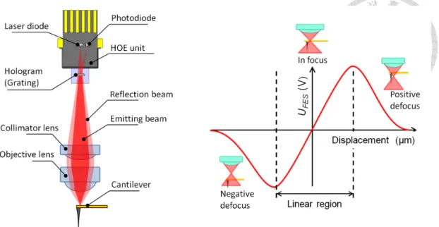
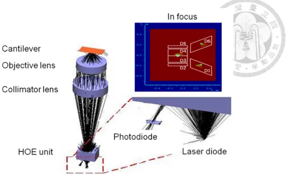
Figure 2.5 represents the configuration of the holographic pickup head which consists of a HOE unit, collimator lens and objective lens. Through the collimator lens and objective lens, the emitting beam of the laser diode is focused on the AFM cantilever. The suggested focal length f and numerical aperture NA of the objective lens of the pickup are 3.3 mm and 0.6. For a measuring system, the focal length and numerical aperture of the collimator lens are 19.07 mm and 0.13. Figure 2.5(b) shows the translational S-curve, which represents the relationship between the focus error signal UFES and the defocus displacement of the detected surface. In the linear region, the UFES is proportional to the cantilever translational displacement.

Figure 2.5 Configuration and translational S-curve of holographic pickup head

2.2 Theoretical Analysis of HOE 2.2.1 Ray-tracking of diffracted beam

In physics, ray-tracking method[35] can be used to calculate the beam conditions of propagating in medium. Any combination of four things might happen with this light ray:

absorption, reflection, refraction and fluorescence. The idealized beam is calculated to explain the real optical device. In order to comprehend the properties of the holographic pickup head, the ray-tracking method is applied. Figure 2.6 illustrates the schematic diagram of the holographic pickup head.

Figure 2.6 Schematic ray-tacking of holographic pickup head

In the simplified optical system, the laser beam is transmitted through the labeled points O, P, Q, R, S, T, U, V and W on the holographic plate as and creates some skew rays respectively. Each labeled point is denoted as a known point (X0, Y0, Z0) on each skew ray, and its direction cosines vector are defined as K, L, and M

X K D X   0 (2.3) Y   L D Y0 (2.4)

( 0 )

Z M D   Z d (2.5) where D is the distance from the object point (X0, Y0, Z0) to the point of incidence (X, Y, Z), and d is the distance between the collimator and the objective lens. For a sphere of the radius r, the equation of the next refracting surface is X²+Y²+Z²-2rZ=0. Substituting Eqs.

(2.3-2.5) in the formula gives the equation to be solved for D as

2 2 0

D  rF D rG   (2.6) where





F K r

  

  (2.7)

2 2 2

0 0 0

0

( )

2( )

X d Y Z

G X d

r

  

   (2.8)

The solution is,

2 1/2

( G)

D r F F r

 

     (2.9)

D must always be positive. If the value of D is solved, return to Eqs.(2.3-2.5) and calculate the coordinates of the point of incidence. The property of direction cosines that the angle between two intersecting lines is given by

cosI Kk'Ll'Mm' (2.10) here, I is the incidence angle and k’, l’, m’ are the direction cosines vectors of the

normal at the point of incidence. For a spherical surface

' X

k   r (2.11)

' Y

l   (2.12)

' 1 Z

m   r (2.13) In order to derive the refraction equations, Figure 2.7 displays the refraction of a skew ray. OA is a vector of magnitude n in the direction of the incident ray, OB is a vector of magnitude n’ in the direction of the refracted ray, while AB is a vector of magnitude n’cosI’-ncosI in the direction of the normal. Substituting Egs.(2.11-2.13) in Eq.(2.10), the value of incidence angle I and refraction angle I’ are obtained.

Figure 2.7 Refraction of skew ray [35]

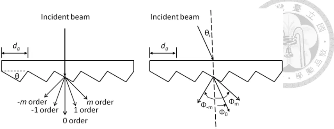
For the holographic optics, the light beam is diffracted by the surface grating. Figure 2.8 shows transmission grating diffracted orders and blazed transmission grating. For transmission gratings at normal incidence, the diffracted orders governed by the following equation

(sin sin )

g i m

md    (2.18)

where m is the order of the diffracted wave, λ is the diffracted wavelength (650 nm), dg is the groove spacing (54.982 µm), θi is the incidence angle, φm is the angle of diffraction of the m order measured from the grating normal.

Figure 2.8 Transmission grating diffraction

The gratings are commonly used with oblique incident angles. Figure 2.9 illustrates the diffraction process on a holographic grating plate, and a unit sphere is applied to describe the relation between the incident ray and the diffracted beam[36]. Every point on the unit sphere may correspond to a point on the α-β plane. The incident ray has an incident point of (αi, βi), and the diffracted ray has an outcoming point of (αm, βm). The diffraction order m is decided by the outcoming point (αm, βm), which can be mapped on one of the orthogonal planes parallel to the grating grooves.

The direction cosine diagram provides a simple and intuitive means of determining the diffraction grating behavior even for these general cases. The general grating equation for arbitrarily oriented lines is given by

m i sin

g

m d

     (2.19)

m i sin

g

m d

      (2.20)

where  is the angle between the direction of the grating grooves and the  -axis.

Therefore from each diffracted ray, the projected spot coordinate (X, Y) on the photodiode can be calibrated by the direction cosine space. Through these mentioned equations by the ray-tracking method, the approximate spot shape variation on the photodiode is derived. Figure 2.10 demonstrates the projected spot on the photodiode coordinate.

Figure 2.10 Projected spot on photodiode coordinate

2.2.2 Spot size and depth of focus

In DVD system, the focus laser spot is actually an area where the intensity of light varies as an airy pattern function. The spot size is determined by the light wavelength λ and the numerical aperture NA of the lens. Therefore, a simple formula is given to calibrate the radius of the focus laser beam by

0.61 Spot size

NA

  (2.21)

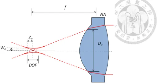
A commercial DVD pickup head uses the red laser (λ=650 nm), the NA of the objective lens is 0.6. The diameter of spot size is 1.32 μm. However, in optics, the laser beam is a Gaussian beam. The aperture diameter is defined as 1/e² (=0.135) of its maximum intensity value on the optical axis. For a Gaussian beam propagating in free space, a laser beam converges to a point where the beam is the smallest, known as the beam waist W0. The beam waist can be regarded as the minimum spot size. Besides, the depth of focus (DOF) is the distance range between the nearest and the farthest objects in a scene that appears acceptably sharp in an image. It can be defined from Rayleigh length ZR[37], which is the distance from the waist to the place where the cross section area is double.

Figure 2.11 illustrates the characteristics of a laser beam through a focusing lens. The beam waist and depth of field can be derived by the following equations, where f is the focal length and D0 is the diameter of the entrance pupil.

0 0

W 2 f D



 (2.22)

2 0 R

Z W

  (2.23)

2

2 0

2 _R W

DOF Z 

   (2.24)

Figure 2.11 Focusing path of laser beam

The numerical aperture of objective lens brings significant influence on lateral resolution. Figure 2.12 illustrates the effect of numerical aperture on the desirable lateral resolution[38]. An objective lens with low numerical aperture NA generates a bigger beam waist, resulting in relatively long DOF. A high numerical aperture NA objective lens induces a smaller beam waist, leading to relatively shorter DOF. Besides, the distance from focal plane to de-focal plane is directly proportional to the DOF.

Figure 2.12 Effect of numerical aperture on lateral resolution

2.2.3 Optical analysis in liquid

Figure 2.13 shows how the optical path changes when the optical system applies in liquid environment. The objective lens doesn’t contact the liquid directly. A cover glass is placed between air and liquid to avoid scattering by a cambered liquid surface and create a clear window. And the relationship between the angles of incidence and refraction can be formulated by Snell's law.

Figure 2.13 Focusing path of laser beam in liquid

In order to know the focus position in liquid, the thickness from the focal point to the surface of the liquid is defined as hliquid, the thickness of the glass is hglass, and the length form the airy focal point to the top surface of the glass is hair. In optics, the numerical aperture of an optical system such as an objective lens is defined by NA=nsinθ. Where n is the index of refraction of the medium and θ is the half-angle of the maximum cone of light that can enter or exit the lens. Due to Snell's law, the numerical aperture remains the same:

sin sin sin

air air glass glass liq liq

NA n  n  n  (2.25) where nair is the refractive index of the air (=1), nglass is the refractive index of the glass (=1.52), nliq is the refractive index of the liquid (e.g. 1.33 for pure water). The θair, θglass, and θliq are the half-angles of the medium. The incident spot which is on the top surface of the glass is the same both in air and in liquid, the equation should be satisfied:

tan tan tan

air air glass glass liquid liq

h  h  h  (2.26)

  

2.3 Simulation of HOE

2.3.1 Focus error signal and translational deflection

Figure 2.14 displays the definition of deflections. The translational deflection Sz deforms along the Z-axis. The angular displacement θx along the torsional direction and θy along the bending direction deflect around the X-axis and Y-axis of the cantilever, respectively.

Figure 2.14 Definition of deflections

The software LightTools is used to analyze the laser shape on the photodiode. When the laser beam is perfectly focus on the detected surface, the reflected laser beam on the six-segment photodiode is symmetric. The simulation explains the translational S-curve of focus error signal UFES that is produced with the adopted collimator and objective lens.

Figure 2.15 shows the construction of simulation optical setup and the result of light spots on the photodiode when the cantilever is in focus.

Figure 2.15 Optical simulation model

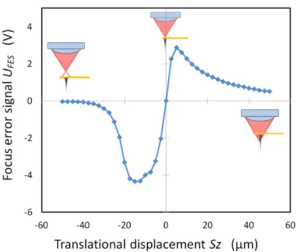
Figure 2.16 illustrates the simulation results of the reflected spots on the photodiode when the cantilever deflects with translational displacement Sz from -20 to 20 μm. The energy distributions on the photodiode are computed. Figure 2.17 shows the relationship between the focus error signal UFES, and translational displacement Sz, the translational S-curve which is calibrated. The simulated translational S-curve is not symmetrical as the result of the different diffuse velocities of the oblique beam cone when the cantilever is at a de-focal position.

Figure 2.16 Simulated spots on photodiode for translational displacement Sz from -20 to

Figure 2.17 Relationship between focus error signal UFES and translational displacement Sz

2.3.2 Tracking error signal and torsional signal

Two other types of angular deflections of cantilever, the torsional deflection around the X-axis and the bending deflection around the Y-axis, are also comprehensively studied.

Figure 2.18(a) represents the simulation results of the reflected spots on the photodiode when the cantilever is deflected by bending angle θy from 1° to 20°. Figure 2.18(b) shows the results for bending angle θy form -1° to -20°. The energy distributions on the photodiode are computed. Figure 2.19 shows the relationship between the tracking error signal UTES, and bending angle θy, the bending S-curve which is calibrated.

Figure 2.18 Simulated spots on photodiode for different bending angles

Figure 2.20 represents the simulation results of the reflected spots on the photodiode when the cantilever is twisted by torsional angle θx from -20° to 20°. The simulation results show the deformations of the beam profiles that are changed with the right side segments (D1+D6) and left side segments (D2+D3+D4+D5). Computed the energy distributions on the photodiode, the output voltage signal from the six-segment photodiode is defined

2 3 4 5 1 6

( ) ( )

TR D D D D D D

U  U U U U  U U (2.28)

Figure 2.21 represents the relationship between the torsional signal UTR, and torsional angle θx of the cantilever, the torsional S-curve which is calibrated.

Figure 2.20 Simulated spots on photodiode for different torsional angles

Figure 2.21 Relationship between torsional signal UTR and torsional angle

2.3.3 Translational S-curve in air and water

For simulating the translational S-curve of focus error signal UFES in water, a model is built up by the software LightTools shown in Figure 2.22. The cantilever is immersed in 1 mm thick water layer, which is covered by a 0.2 mm cover glass with reflective index of 1.515.

Figure 2.22 Optical simulation model in water

Figure 2.23 shows the simulated translational S-curves in air and water. From the schematic diagram of theoretical analysis (shown in Figure 2.13), the incidence angle is smaller than in air. The effect is similar to an objective lens with smaller numerical aperture. Therefore, the linear region in water will be longer than in air. In the simulation, the peak to peak voltage of the translational S-curve is form 7.22 V in air to 5.26 V in water. The voltage is reduced by 27%. The linear region is increased by 42% that from 12 μm in air to 17 μm in water. The slope of linear region in water is slower than in air, the sensitivity is from 0.60 to 0.31 V/μm, which is lower than in air.

Figure 2.23 Simulated translational S-curve in air and water

2.4 Cantilever Dynamics

2.4.1 Cantilever dimensional effect

Figure 2.24 illustrates the geometric dimensions of a rectangular cantilever. When considering the behavior of the cantilever in liquid, the spring constant k only depends on the material properties of the cantilever and its geometrical dimensions. The formula for the spring constant of a cantilever is defined:

3 3

k Eh w

 l (2.29)

Figure 2.24 Geometric dimensions of rectangular cantilever

where E is Young's modulus of the material and h, w, l are the thickness, width, and length of the cantilever, respectively. However, viscosity of the surrounding media does affect the mechanical response of the cantilever, especially in liquid. The movement of a cantilever driven by an external oscillatory force F(t)=F0cos(ωt) can be described as a forced harmonic oscillator with damp[39].

0cos( )

m z kzg   





0

mg

Q

   (2.31)

0 2

(1 1 )

r 2

   Q (2.32)

Here, z is the vertical movement of the cantilever, mg is its mass, ω0 is its free resonant frequency and ωr is its resonant frequency in a fluid, Q is the quality factor, γ is the damping coefficient, and F0 is the amplitude of the oscillatory force at a time t.

If according to the Euler-Lagrange equation[40], the elastic deformation of the cantilever executing flexural oscillations is expressed as:

4 2

4 2

( , ) ( , )

( , )

w x t w x t

EI F x t

x  t

   

  (2.33) where w(x,t) is the deflection function of the cantilever in the Z-axis direction, I is the moment of inertia of the cantilever cross section, μ is the mass per unit length in Z-axis direction, x is the spatial coordinate along the length of the cantilever. For a rectangular cantilever beam, I=wh³/12 and μ=ρcwh, where ρc is the cantilever density. To calculate the frequency response of the cantilever, Fourier transform of this governing equation is taken. Solving equations in the absence of any applied load leads to the result for the vacuum radial resonant frequency (ωvac)[41]

2 2

2 12 2

n n

vac

c

C EI C h E

l l

 ^  ^  (2.34)

where n is the mode order and Cn is the nth positive root of 1+cosCncoshCn=0.

Sader introduced a hydrodynamic load into the equation of the elastic deformation[42].

The dynamic equation becomes

4

2 4

( , )

( , ) ( , )

c

EI w x wh w x F x

x     

  

 (2.35)

where ω represents the vibrational frequency, and the external force is distinguished into two components.

( , ) _hydro( , ) _drive( , )

F x F x  F x (2.36) where Fhydro(x,ω) is the hydrodynamic load exerted by the fluid, and Fdrive(x,ω) is the

driving forces that excites the cantilever. Based on the equations of motion for liquid, the general form of Fhydro(x,ω) is given by

2 2

( , ) ( , Re) ( , )

hydro 4 f

F x    w  k w x  (2.37) where ρf is the fluid density, and Γ(k.Re) is the dimensionless hydrodynamic function, which depends on the Reynolds number Re=ρωw/η and the aspect ratio k=Cnw/l, where η is the fluid viscosity. For calculating the resonant frequency in fluid, Fdrive(x,ω) and dissipative effects are neglected. Therefore, the relation between the resonant frequency in fluid and vacuum is expressed as:

1/2

1 ( , Re)

4

r f

r vac

w k

h

 

 

 

   

  (2.38) and the Q-factor is

(4 / ) ( , Re)

( , Re)

f r

i

h w k

Q k

   

  (2.39)

The longer cantilever has smaller spring constant k, and its resonant frequency ω and Q-factor are also lower. If broadening the width of the cantilever can increase the Q-factor, but ω will be reduced and k will be raised. If increasing the thickness of the cantilever, both ω and Q-factor will be increased, but k will be raised. Therefore, ω, Q, and k can’t be directly improved at the same time through modifying any single dimension of the cantilever[43].

2.4.2 Cantilever dynamics in air and water

According to the Equations (2.33) and (2.38), the resonant frequency and Q-factor of the AFM cantilevers are calculated. A longer cantilever (PPP-CONT, Nanosensors) for contact mode AFM and a shorter cantilever (PPP-NCH, Nanosensors) for tapping mode AFM are adopted for

Table 2.1 Parameters of theoretical analysis

PPP-NCH PPP-CONT

Length l 125 μm 450 μm

Width w 30 μm 50 μm

Thickness h 4 μm 2 μm

Density of air



Viscosity of air



Density of water



Viscosity of water



Temperature T 298 K

Density of cantilever



Young’s modulus E 170 GPa

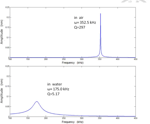
According to the theoretical derived frequency spectrum of PPP-NCH in air, its resonant frequency and Q-factor are 352.5 kHz and 297, respectively. In water, the resonant frequency and Q-factor are 175 kHz and 5.17, respectively. The resonant frequency in water is decreased by 50% than in air. The quality factor declines form 297 to 5.17. Figure 2.25 demonstrates the theoretical derived amplitude spectra.

Figure 2.25 Analytical amplitude spectra of PPP-NCH in air and water

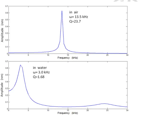
In air, resonant frequency and Q-factor of the frequency spectrum of PPP-CONT are 13.5 kHz and 23.7, respectively. In water, the resonant frequency and Q-factor become 3 kHz and 1.68. The resonant frequency in water is dropped off by 78% than in air. The quality factor declines form 23.7 to 1.68. Figure 2.26 demonstrates the analytical amplitude spectra. Through the results of theoretical verification, the resonant frequency and quality factor are reduced in water.

Figure 2.26 Analytical amplitude spectra of PPP-CONT in air and water