改良式粒子群最佳化求解具接駁式轉運之車輛運途問題研究

(1)

行政院國家科學委員會專題研究計畫成果報告

改良式粒子群最佳化求解具接駁式轉運之車輛運途問題研究

研究成果報告(精簡版)

計畫類別：個別型

計畫編號： NSC 100-2410-H-011-029-

執行期間： 100 年 08 月 01 日至 101 年 07 月 31 日執行單位：國立臺灣科技大學工業管理系

計畫主持人：羅士哲

計畫參與人員：碩士班研究生-兼任助理人員：莊英林碩士班研究生-兼任助理人員：陳偉剛碩士班研究生-兼任助理人員：王詠賢碩士班研究生-兼任助理人員：涂瑋哲

公開資訊：本計畫可公開查詢

中華民國 101 年 09 月 30 日

(2)

中文摘要：一個經濟且具效率的物流作業可以讓一個公司能夠快速回應客戶的需求，因此能在眾多競爭者之中獲取競爭優勢。隨著過去幾年的經濟不景氣，全世界有更多的企業把注意力集中到供應鏈管理與全球運籌管理的領域之中。在本研究之中，

我們設計一個創新的混合式演算法，來找出具接駁式轉運之車輛運途問題的組合最佳化問題解。我們所提出之演算法將以粒子群最佳化為核心，搭配掃描法作為分群演算法，以快速找出近似最佳解。本研究所提之演算法將與傳統之基因演算法作比較，並應用修改之具收送限制之車輛運途問題作為標竿問題，以驗證所提出之演算法效能。實驗結果說明所提之演算法，在 60 個標竿問題中，均能夠比基因演算法找出具接駁式轉運之車輛運途問題的最佳解，且所提之演算法具有強韌、收斂快速與競爭力，以平均解的品質來比較時，比基因演算法改善率達 39.3%。

中文關鍵詞：物流、接駁式轉運、粒子群最佳化、車輛運途問題、掃描法。

英文摘要： An efficient and effective logistics operation

enables a company to quickly respond to a customer’s requirements and thus acquire a competitive edge over its competitors. With economic depression spreading around the world for the past few years, enterprises are paying great attention to supply chain management and global logistics management around the world. In this research, we are going to design a novel

algorithm to find the combinatorial optimal solution for the vehicle routing problem with Cross-docking in a supply chain. The proposed algorithm is based on the particle swarm optimization (PSO) algorithm combined with the sweep method to quickly generate a near-optimal solution. Comparisons between the

proposed method and the genetic algorithm (GA) by performing experiments involving modified VRP pickup and delivery benchmark problems to validate the performance. Experimental results showed that the sPSO method was able to find solutions with lower costs than the GA method for all the 60 benchmarks applied. Moreover, the computational results show that the sPSO algorithm is robust, converges quickly, and is competitive, with an average improvement of 39.3% over the GA method in terms of the average

(3)

solution quality.

英文關鍵詞： Logistics； Cross-docking； Particle swarm optimization； Vehicle routing problem； Sweep method.

(4)

0

行政院國家科學委員會補助專題研究計畫行政院國家科學委員會補助專題研究計畫行政院國家科學委員會補助專題研究計畫

行政院國家科學委員會補助專題研究計畫 □ □ □ □ 期中進度報告期中進度報告期中進度報告期中進度報告

■

■ ■ 期期期末期末末報告末報告報告報告

改良式粒子群最佳化求解具接駁式轉運之車輛運途問題研究

On the Study of Improved Particle Swarm Optimization to Solve the Vehicle Routing Problem with Cross-docking

計畫類別：■■■■ 個別型計畫 □ 整合型計畫計畫編號：NSC 100 - 2410 - H - 011 - 029 -

執行期間： 100 年 08 月 01 日至 101 年 07 月 31 日執行機構及系所：國立臺灣科技大學工業管理系(所)

計畫主持人：羅士哲

計畫參與人員：莊英林、陳偉剛、王詠賢、涂瑋哲

本計畫除繳交成果報告，另包括下列出國報告，共 0 份：

□移地研究心得報告一份

□出席國際學術會議心得報告

□國際合作研究計畫國外研究報告

處理方式：除列管計畫及下列情形者外，得立即公開查詢

□涉及專利或其他智慧財產權，□一年□二年後可公開查詢

中華民國 101 年 9 月 30 日

(5)

0

因此能在眾多競爭者之中獲取競爭優勢。隨著過去幾年的經濟不景氣，全世界有更多的企業把注意力集中到供應鏈管理與全球運籌管理的領域之中。在本研究之中，我們設計一個創新的混合式演算法，來找出具接駁式轉運之車輛運途問題的組合最佳化問題解。我們所提出之演算法將以粒子群最佳化為核心，搭配掃描法作為分群演算法，以快速找出近似最佳解。本研究所提之演算法將與傳統之基因演算法作比較，並應用修改之具收送限制之車輛運途問題作為標竿問題，以驗證所提出之演算法效能。實驗結果說明所提之演算法，在 60 個標竿問題中，均能夠比基因演算法找出具接駁式轉運之車輛運途問題的最佳解，且所提之演算法具有強韌、收斂快速與競爭力，以平均解的品質來比較時，比基因演算法改善率達 39.3%。

關鍵詞關鍵詞關鍵詞

關鍵詞：：：：物流、接駁式轉運、粒子群最佳化、車輛運途問題、掃描法。

英英英

英文摘要文摘要文摘要文摘要

An efficient and effective logistics operation enables a company to quickly respond to a customer’s requirements and thus acquire a competitive edge over its competitors.

With economic depression spreading around the world for the past few years, enterprises are paying great attention to supply chain management and global logistics management around the world. In this research, we are going to design a novel algorithm to find the combinatorial optimal solution for the vehicle routing problem with Cross-docking in a supply chain. The proposed algorithm is based on the particle swarm optimization (PSO) algorithm combined with the sweep method to quickly generate a near-optimal solution. Comparisons between the proposed method and the genetic algorithm (GA) by performing experiments involving modified VRP pickup and delivery benchmark problems to validate the performance. Experimental results showed that the sPSO method was able to find solutions with lower costs than the GA method for all the 60 benchmarks applied. Moreover, the computational results show that the sPSO algorithm is robust, converges quickly, and is competitive, with an average improvement of 39.3% over the GA method in terms of the average solution quality.

Keywords: Logistics; Cross-docking; Particle swarm optimization; Vehicle routing problem; Sweep method.

(7)

2

(三)

報告內容

1. Introduction

With economic depression spreading around the world, enterprises are paying great attention to supply chain management (SCM) and global logistics management.

One of the most important factors involved in implementing SCM is the efficient control of the physical flow of the supply chain. An efficient and effective logistics operation enables a company to quickly respond to a customer’s requirements and thus acquire a competitive edge over its competitors. In fact, logistics costs have a significant effect on a company’s total production and distribution costs. For example, transportation costs account for one thirds to two thirds of a company’s overall distribution cost in general. LaLonde and Zinszer (1976) showed that logistics costs account for approximately 10% of a company’s revenue, while Apte and Viswanathan (2000) argued that 30% of the final cost is incurred in the distribution process. In order to lower costs, increase profits, and improve a company’s overall performance, a well-organized and highly efficient logistics network appears to be essential.

Therefore, a Cross-docking (CD) system in the supply chain is considered to be a good method to reduce inventory and improve the responsiveness to various customer demands.

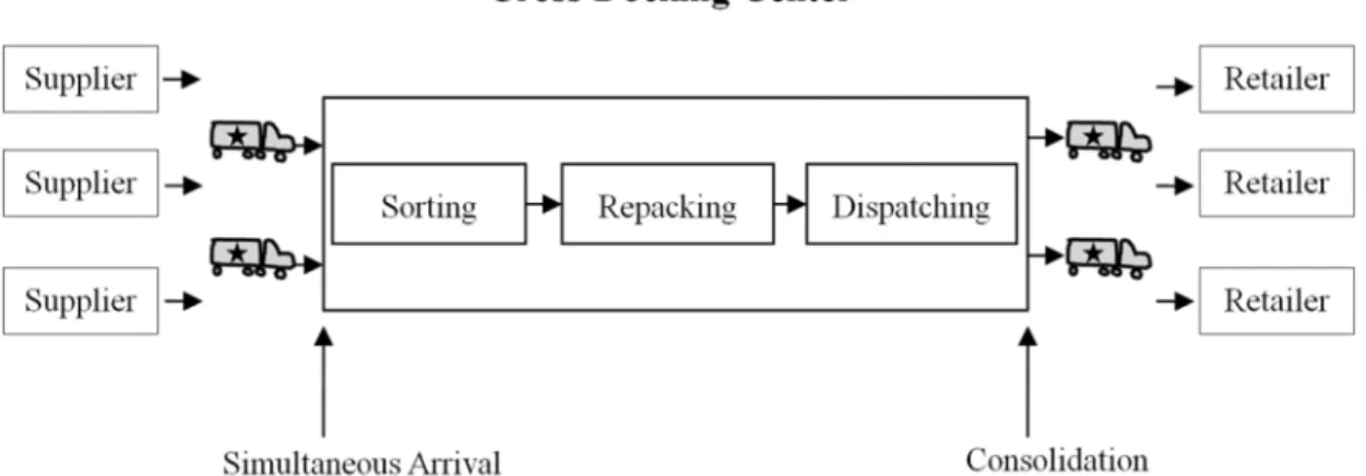
Cross-docking is the concept of keeping goods moving from the time they are received to shipping without ever storing them in a warehouse. It is also considered to be the optimal vehicle routing for the associated direct service fulfillment, subject to loading capacity and service time constraints (Sung and Song 2003). The primary objective is to avoid the inventory and handling costs; thus, ideally, no inventory is stored in the central warehouse. One of the earliest technical papers on Cross-docking systems was presented by Rohrer (1995). He stated that a successful Cross-docking system can bring companies significant benefits, including inventory reduction, low space requirements and transportation costs, increased customer responsiveness, and better control of the distribution process. Figure 1 shows the typical layout used in a Cross-docking operation. The physical flow of goods from suppliers to retailers is collaboratively optimized during both the pickup and delivery processes in order to achieve the no inventory and no delayed shipment scenario to reduce the overall transportation costs and increase customer satisfaction.

(8)

3

Figure 1. A layout of the typical Cross-docking system.

This paper focuses on solving the vehicle routing problem with Cross-docking.

To effectively implement the Cross-docking system in a logistics network, the receiving (pickup) and shipping (delivery) processes must be considered at the same time. Lee et al. (2006) argued that the core issue in the pickup process is that all the routing vehicles must arrive at the Cross-docking depot simultaneously. In other words, a vehicle that returns early has to wait at the depot until all the other vehicles arrive from their pickup tasks. In addition, the amount of products arriving from suppliers has to equal to the amount of products ready to be delivered to customers from the depot. Then, through the sorting, repacking, and dispatching processes in the Cross-docking warehouse, the designated shipments are loaded on vehicles for delivery to their respective destinations. Moreover, in order to minimize the total operation time or maximize the throughput of the Cross-docking system, Yu and Egbelu (2006) studied a Cross-docking system with a temporary storage area in front of the dispatching dock. Their primary objective was to find the best truck docking sequence for both inbound and outbound trucks. Celik et.al (2009) studied ship docking facilities by using Fuzzy method to evaluate operation performance.

Because the VRPCD is a well-known non-deterministic polynomial-time hard (NP-hard) problem, applying an efficient heuristics technique is necessary in order to obtain the best or near-optimal solution within a reasonable amount of computation time. Bell and Mcmullen (2004) proposed a modified ant colony optimization (ACO) to solve vehicle routing problems and found that the proposed multi-ACO algorithm is competitive in terms of computation time, particularly when the number of customers is large. Mosheiov (1998) dealt with the pickup and delivery VRP using tour-partitioning heuristics. The goal was to obtain the optimal set of vehicle routes as well as to minimize the total traveling distance. Zachariadis et al. (2010) dealt with the vehicle routing problem with simultaneous pickup and delivery (VRPSPD) using

(9)

4

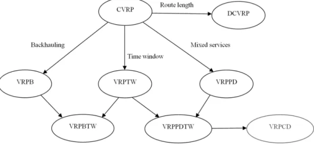
adaptive memory (AM) algorithm, which proved to be more effective and efficient than other heuristics. Furthermore, they found some new best known solutions of the numerous VRPSPD instances. Lai and Cao (2010) proposed an improved differential evolution algorithm (IDE) for solving the vehicle routing problem with simultaneous pickups and deliveries and time windows (VRP-SPDTW) and showed that the proposed method is effective for solving VRP-SPDTW. Figure 2 shows an example of the basic VRP problems with various constraints (Toth and Vigo 2001).

Figure 2. The basic VRP problems with various constraints.

In this paper, we proposed a novel algorithm, called sPSO, based on particle swarm optimization (PSO) to solve vehicle routing problems using the practical concept of Cross-docking in logistics networks. PSO is a newly developed evolutionary meta-heuristics in the field of swarm intelligence. It was introduced by Kennedy and Eberhart (1995) based on observations of a simplified social model for bird flocks. Shi and Eberhart (1998a; 1998b) introduced a newer version of PSO by adding an inertia weight, W, to the original PSO equation. The authors argued that this inertia weight plays a role in balancing between local search and global search.

Furthermore, they proved that a PSO with average inertia weight values ranging from 0.9 to 1.2 generates a better performance. On the other hand, a discrete binary version of the PSO was presented by Kennedy and Eberhart in 1997. The concept of the PSO function remains the same, except that the trajectories are changed in terms of probability. Lately, MirHassani and Abolghasemi (2011) applied the pure PSO algorithm to solve for open vehicle routing problem, while Marinakis, and Marinaki (2010) combined the genetic algorithm and the PSO Algorithm together into a hybrid model for the vehicle routing problem.

This paper is organized as follows. Section 2 presents the problem formulation.

The procedure for the sPSO algorithm is described in Section 3. Section 4 shows the

(10)

5

computational experiments and provides an analysis of the results. Section 5 concludes the paper with a summary.

2. Problem Formulation

This section defines problem proposition of the VRP with the constraints of a Cross-docking system. In the problem of vehicle routing with one Cross-docking hub constraints defined by Lee et al. (2006), the Cross-docking center plays a key role in synchronizing the distribution process on both sides of supply chain. In simulations, the Cross-docking hub can be treated as the home depot as in traditional vehicle routing problems, except the Cross-docking model specifies for the simultaneous arrival of each vehicle from receiving trips, as well as the transportation of equivalent quantities of goods on both sides of the supply chain. Therefore, several assumptions are made. First, we have n nodes comprising both suppliers and retailers, serviced by m vehicles. These vehicle must be dispatched from the Cross-docking hub (i = 0) and arrive back at the same time. In addition, there is only one Cross-docking hub allowed and the total amount of goods collected from suppliers must equal the quantity ready for delivery to retailers. Moreover, for computational convenience, the service time δ is set to zero.

Second, for each customer, only one vehicle is assigned with one route, and is associated with a cost amount cij, which represents the travel distance from node i to j.

Moreover, every customer has the same amount of demand d, which is restricted to the capacity limit q of each vehicle. There is also a time horizon T which specifies the total distance that can be traveled by vehicles without exceeding it. Two types of cost, taken from both the receiving and delivering routes, are taken into consideration: the transportation cost and operational cost. The overall goals are to obtain the optimal routing schedule and to determine the number of vehicles used, and total cost minimization with shortest traveling distance. The following paragraph presents the decision variables of the VRPCD formulation.

Basic notations:

Xijk : a binary variable representing the route from i to j is serviced by vehicle k.



=

otherwise.

, 0

; to from tour in the is vehicle if

,

1 k i j

X_ijk

Yijk : loaded quantity of vehicle k from pickup trip i to j.

Zijk :unloaded quantity of vehicle k from delivery trip i to j.

tcijk :the transportation cost of vehicle k from customer i to j.

etijk : time for vehicle k to move from i to j.

δ_ik: service time required by vehicle k to load/unload the quantity demand at i.

m: number of vehicles.

n: number of customers.

(11)

6

ck : fixed cost of vehicle k.

qi : maximum capacity for each vehicle.

T: planning horizon.

P: unit demand from each pickup stop.

D: unit demand from each delivery stop.

DT: departure time.

AT: arrival time.

Objective function:

∑ ∑ ∑ ∑ ∑

= = = + = =

= ⁿ

i n j

m k

n j

jk k ijk

ijX c X

tc

0 0 1 1 1

Z 0

Minimize (1)

Subject to:

; ..., 2, , 1 for , 1

0 1

n j

X

n

i m

k

ijk = =

∑∑

= =

(2)

; ..., 2, , 1 for , 1

0 1

n i

X

n

j m

k

ijk = =

∑∑

= =

(3)

; 2,..., , 1 , ..., 2, 1, for ,

1 1

n h

m k

X X

n

j hjk n

i

ihk =

∑

= =

∑

=

(4)

∑

=

n ≤

j

jk k m

X

1

0 1,for 1,2,..., ; (5)

∑

=

n ≤

i k

i k m

X

1

0 1, for 1,2,..., ; (6)

∑ ∑

= =

=

≤

+ ⁿ

i n

j ijk i ijk

ijk Z q X k m

Y

1 1

; 2,..., 1, for

, (7)











=

∈

−

=

∈

=

∈

=

−

∑

=

; 2,..., 1, , 0 if ,

, 2,..., 1, , if ,

0

, 2,..., 1, , if ,

1

n i

j P

n i

D j

n i

P j P

Y Y

n

i i j ijk jik

(8)











=

∈

=

∈

=

∈

=

−

∑

=

; 2,..., 1, , 0 if ,

, 2,..., 1, , if ,

, 2,..., 1, , if 0,

1

n i

j D

n i

D j D

n i

P j Z

Z

n

i i i jik ijk

(9)

∑ ∑ ∑ ∑

= = = =

=

≤

n +

i n

j

n

i n

j

ijk ijk ijk

ikX et X T k m

δ

0 0 0 0

; 2,..., 1, for

, (10)

(

^et ^DT ^δ

)

^X ^,^for^k ^1,^2,...,^m^;

DT_jk= _ijk+ _ik+ _j _ijk = (11)

(et0 DT )X 0 ^,^fork ^1,^2,...,m^;

AT_k = _i _k + _ik _i _k = (12)

. for

, ^'

' k k

AT

AT_k = _k ≠ (13)

(12)

7

Equation (1) states that the overall objective is to minimize both the transportation cost and fixed cost. Equations (2) and (3) indicate that each customer is serviced by only one vehicle, while Equation (4) states that each vehicle arriving at a node must also leave from that node. The vehicle constraints that only allow a vehicle to start from and return to the Cross-docking hub and ensure that it is used to serve at most one route are shown in (5) and (6), respectively. Equation (7) specifies that the loading and uploading demands from the pickup and delivery processes cannot exceed the vehicle quantity limit, while Equations (8) and (9) detail these quantity limits for the pickup and delivery processes. The total distance traveled and time consumed cannot exceed the planning horizon, as specified in Equation (10).

Equations (11) and (12) state the departure and arrival times, respectively. Equation (13) constrains the simultaneous arrival of vehicles at the Cross-docking hub.

3. The sPSO Method

Section 3.1 presents the methodology of the sPSO method, which is followed by the detailed procedure for the algorithm in section 3.2

3.1 Methodology

Each dispatched vehicle has to serve the maximum number of customers under its capacity limit with the minimum travel distance in order to minimize the total cost.

In this study, we simulate a practical strategy using the PSO algorithm to solve the problem and generate a vehicle routing sequence with one Cross-docking operation in the supply chain. However, past researches have indicated that the PSO method is fast but has premature convergence. Moreover, the final solution quality will be improved if the initial solution for the PSO is prominent. Therefore, a clustering algorithm, called the sweep method, was introduced to group customers in the beginning of the proposed algorithm.

Usually the sweep method is applied to a polar coordinate system, where the center of the coordinate system served as the depot in a vehicle routing problem.

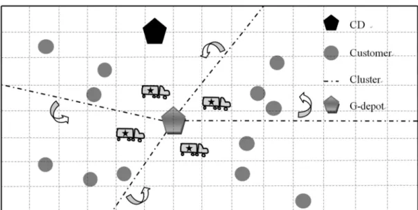
However, in order to obtain the maximum performance from the sweep method, the center of gravity for all the customers is set as the center of the coordinate system in this study, called the G-depot. Customers are joined to the G-depot one by one depending on vehicle capacity to determine the number of vehicles. The initial solution for the sPSO algorithm from the sweep method is generated by the following methodology.

For each traveling distance of route Oi (i = 1, 2, …, N, where N is the number of customers), the ith customer’s Ci serves as the first customer in the cluster. Next, we search for the closest customer to Ci, Ci+1, by increasing the angle. This is then added to the same cluster if it can be done without exceeding the vehicle capacity. When a

(13)

8

customer cannot be added to current cluster due to the vehicle capacity limit, this customer becomes the first customer of the next cluster. This process is repeated until all the customers are assigned. Figure 3 illustrates the clustering process for several nodes. The dotted straight lines represent the sweep hand moving counter clockwise.

After all the customers are grouped, we calculate the objective value of this route.

After O1, O2, …, ON, are calculated, we chose the minimum N route distance as the initial solution of the sPSO algorithm. That is,

Initial solution = min{Oi}, for i = 1, 2, …, N.

Figure 3. An example of cluster by sweep method.

Customers that are located close to each other are grouped into the same cluster.

This makes it possible to generate the fewest number of vehicles used and reduce the operational cost. Next, the initial solution of the sPSO algorithm is acquired by using the sweep method to search for a global optimal solution.

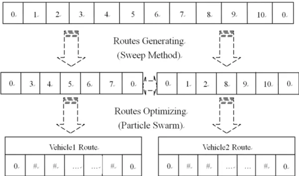
In any set of transport routes, at least one vehicle will be dispatched to serve one master route based on the principle of the sweep method and the minimum distance traveled. The total cost is found by adding the fixed costs for the vehicles used (operational costs) and the transportation costs as vehicles travel from one customer to another. In some cases, the aggregated service time consumed by each customer is also taken into account. Overall, when vehicles travel shorter distances, they incur lower total cost. Figure 4 illustrates the hierarchy of the proposed algorithm with 10 nodes served by 2 vehicles under the scenario of homogeneous demand.

(14)

9

Figure 4. An example of 10 nodes with homogeneous demand served by 2 vehicles.

As shown in Figure 4, in the routes generating phase, the sweep method is defined to construct the clusters and minimize the travel distance in each cluster as an initial route for the next phase. Then, a mapping technique is needed in the routes optimizing phase in order to apply the particles’ continuous flying trail to the discrete solution domain of the vehicle routing problem. Finally, the particle dimension for the PSO is set to the number of all customers served. We also relax the boundary of each cluster to switch customers with clusters in the vicinity in order to ensure that the algorithm to searches all the combinations and generates a better solution quality. The following section details the procedure for the sPSO method.

3.2 sPSO Procedure

The key issue to successfully implementing the sPSO and solving any kind of vehicle routing problems hinges on the representation step. Therefore, a permutation-based representation technique is developed to perform the particle construction phase, which makes it possible to apply the continuous particle domain to the discrete solution of a vehicle routing sequence. We set up the flying field of each particle with the dimension equal to the number of suppliers or customers served.

Thus, the particle dimension represents the positions of the nodes to be visited. In other words, the particle dimension is equal to the length of suppliers’ or customers’

sequences within the routing order.

In the original PSO algorithm, the principles of particle movement contain three major parts. First, inertia weight W resembles the difference in particle coordinates between now and the previous iteration. A larger value of W results in a particle search in more directions (exploration), whereas a smaller value allow the particles

(15)

10

settle into the optima (exploitation). Two learning factors,

id1

ϕ _and ϕ_id₂, denote the tendency of the particles to move toward the individual best (Pbest) and the swarm’s group best (Gbest), respectively. The mechanics of Pbest and Gbest cause individual particles to progressively fly toward the quality solution field. In these cases, each particle is capable of recording its own best flying experience as well as detecting and sharing the knowledge of other particles. The best practice here implies ising whichever permutation set generates the best fitness value.

Based on these characteristics, we propose a new discrete PSO method (sPSO) in this study. The improved sPSO procedure is shown as follows.

), )

) (

(

( ¹ ¹

1

2 id gd

t id t id id

id t

id W X V P P

V =ϕ ϕ ⁻ ⊗ ⁻ ⊗ ⊗ ⁽¹⁴⁾

).

( ¹

3

t id t id id t

id X V

X =ϕ ⁻ ⊗ ⁽¹⁵⁾

The primary principle of the PSO algorithm is learning. Following from this concept, we regard the difference in particle coordinates as a percentage of similarity calculating from the previous coordinates, the individual best and the swarm’s group best. Therefore, we set up four parameters (W,

id1

ϕ _, ϕ_id₂_, ϕ_id₃) as probabilities in Equations (14) and (15), where the inertia weight W inferences the direction from the previous location; the learning factors,

id1

ϕ _and ϕ_id₂ , control the speed of the acceleration the pulls particles toward Pbest and Gbest, respectively; and the third learning factor

id3

ϕ resembles the level of the current position from the velocity. In addition, the notation “⊗” stands for the imitation operator to determine the evolutionary process as described in Table 1.

The movement in direction V_id^t is composed of three parts (previous velocity

−1 t

Vid , individual best Pid, and swarm best Pgd), as shown in (14). The value in the inner parentheses ( ⁻¹⊗ id^t⁻¹)

t

id V

X with the probability of W is calculated from the previous particle and the previous velocity. For every dimensions of a particle, we use a uniform distribution in [0, 1] to generate random numbers. If the random number is less than W, then the dimension of X_id^t⁻¹ is replaced by V_id^t⁻¹, otherwise the current dimension of the particle is kept unchanged. When every dimension of a particle was

(16)

11

checked, the final result is recorded to execute the middle term )

) (

(W X_id^t⁻¹⊗V_id^t⁻¹ ⊗P_id , following the same procedure as for outer parentheses

) ) ) (

(

( ¹ ¹

1 id gd

t id t id

id W X ⁻ ⊗V ⁻ ⊗P ⊗P

ϕ ^. Moreover, the new velocity is used to update the current position, as shown in (15).

Table 1

The Procedure of the sPSO Algorithm.

Step 0: Preparation phase Initialize the parameters

id1

ϕ _, ϕid₂^, ϕid₃, W, swarm size, and max iteration.

Step 1: Generate initial solution

Step 1.1: Calculate gravity of all customers (G-depot).

Step 1.2: All customers are clustered by sweep method.

Step 1.3: Calculate each route distance and denoted as Oi (i=1, …, N).

Step 1.4: Choose the smallest Oi as the initial sequence of the sPSO algorithm.

Step 2: Initialization

For each particle i in the population.

Step 2.1: Initialize particle positions X_id⁰(X_id⁰ =[X_i⁰₁,X_i⁰₂,...,X_id⁰]) generated in Step1.

Step 2.2: Initialize velocity V_id⁰(V_id⁰ =[V_i₁⁰,V_i⁰₂,...,V_id⁰])randomly.

Step 2.3: InitializeP_id⁰(P_id⁰ =[P_i₁⁰,P_i⁰₂,...,P_id⁰]) with a copy of X . _id⁰ Step 2.4: Evaluate Pbest[i].

Step 2.5: Initialize G_best⁰ with the best fitness (fvalue) among the population.

Step 2.6: Calculate P_gd⁰(P_gd⁰ =[P_g⁰₁,P_g⁰₂,...,P_gd⁰]) with the G_best⁰ . Step 3: Repeat till a stopping criterion is satisfied (Going Loop) For each particle i in the population.

Step 3.1: Update velocity by ( ( ( ) ) ).

1 2

1

gd id t id t id id

id t

id W X V P P

V ⁺ =ϕ ϕ ⊗ ⊗ ⊗

Step 3.2: Update position by ¹ ( ¹).

3

+ + = _id _id^t ⊗ _id^t

t

id X V

X ϕ

Step 3.3: Evaluate particle’s fitness (fvalue[i]).

Step 3.4: Determine new P_id^t⁺¹ and new P_gd^t⁺¹ as follows:





≤

= ₊ ₊⁺ >

+

).

( ) ( if

), ( ) ( if

1 1

t id t

id t

id

t id t

id t

id X , f X f P

P f X f , P P





 <

= ⁺ ⁺

+

else.

,

), ( ) ( min if ), ( min

arg ¹ ¹

1 t gd

t gd t

id t

t id

gd P

P f P f P

P f

Step 3.5: Stop when the maximum iteration is achieved; Otherwise, set t=t+1, repeat Step 3.

Step 4: Repeat Step 1-3 for delivery process. Calculate total travel distance.

The learning procedure of the sPSO is based on the three elements described above: previous velocity (V ), individual best P_id^t id, and group best Pgd. Individual

(17)

12

particles are able to attain next quality moves and update their current positions, as shown in Equation (15). Through a process of repeated iterations, the whole swarm of particles moves gradually toward the best position. Table 1 presents the detail of the procedure for the sPSO algorithm.

4. Computational Experiments

A preliminary investigation of the optimal parameters for the sPSO is presented in section 4.1. Sixty VRPPD benchmark problems were retrieved from the VRP Web (http://neo.lcc.uma.es/radi-aeb/WebVRP/index.html) and used as test problems to evaluate the performance of the sPSO methodology as described in section 4.2. The PSO algorithm was programmed via MATLAB on the Window XP platform with a Core 2 Quad 2.4GHz CPU and 4G of RAM. The performance of the sPSO method was compared with that of the Genetic algorithm provided by Evolver 4.0^TM, the Genetic Algorithm Solver plug-in for Microsoft Excel.

4.1 Preliminary Test

In the preliminary experiment, the Design of Experiment (DOE) was initiated to verify the optimal PSO parameter settings for the sPSO approach. Three learning factors

id1

ϕ ,

id2

ϕ , and

id3

ϕ ^, were evaluated through the response surface methodology. The inertia weight W was typically set up to linearly decrease from 1 to 0 during the course using the following equation.

).

( )

( w w

T w t t

w = − − (16)

Here, t represents the current iteration, T stands for the total iterations, and w_and w denote the upper and lower bounds, respectively. The recommended ranges for the three learning factors were derived from the previous literature (Shi and Eberhart 1998b; Hu et al. 2004) in the interval of [0.4, 1.9]. However, four parameters represented probability concept in this study. That is, ^{ϕ_id1^,ϕ_id2^,ϕ_id3^,W^}∈

[ ]

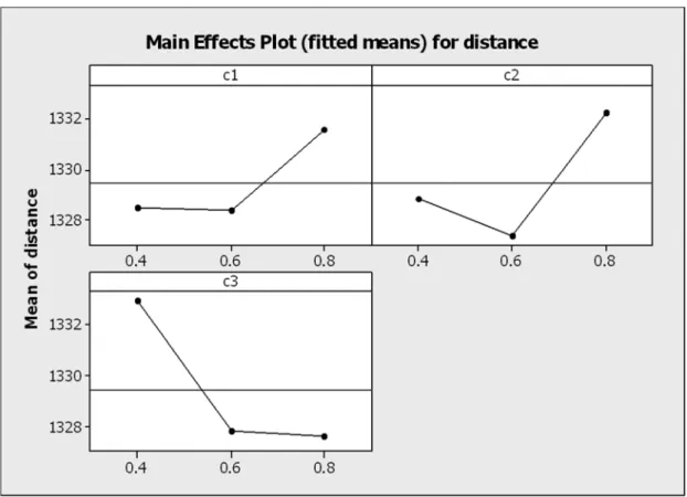
⁰^,¹ . One randomly selected instance from the 60 test problems was used to execute the response surface methodology experiment. Therefore, a 3³ factorial design was constructed, specifying that the three learning factors were set in the range of [0.4, 0.8]

with increments of 0.2. The confidence level was set at 95%.

Figure 5 shows a plot of the main effects of the three factors from the results of the DOE experiment. As shown, c1, c2, and c3 are symbolized as

id1

ϕ ,

id2

ϕ , and

id3

ϕ , respectively. Distance is the response value, representing the average cost generated by different combinations of factor levels.

(18)

13

Figure 5. The main effects plot of factors

2 1, _id

id ϕ

ϕ ^and ϕid₃.

It was observed that the sPSO methodology generated a better solution quality when the learning factors ϕid1_and ϕid₂ were assigned at level 0.6 and ϕid3 _was

assigned at level 0.8. Moreover, the number of particle sizes was given at 200 and the maximum iterations were set at 5000 trials as the termination criterion. These settings were used in the following experiment for the sPSO algorithm. On the other hand, the population size of the genes in the GA method was set at 50 with the mutation rate of 0.06 and crossover rate of 0.15. The maximum iterations were 5000 trials with 30 replications for each instance, applied to both methods.

4.2 Computational Results

The experiment involved 60 datasets of VRP pickup and delivery benchmark problems with the condition of homogeneous demand. Each instance was replicated for 30 runs in the sPSO algorithm. The solution from the sweep method, which generated proper clusters of shipments for grouping vehicles was used as the initial solution for the sPSO method. A performance comparison of the sPSO method and the GA method was computed based on the improvement rate (IR) as shown in Equation (17). The experiment results are given in Table 2.

% GA 100

GA - (IR) sPSO

Rate t Improvemen

cost total

cost total cost

total ×

=

(17)

(19)

14

As listed, the 60 benchmark problems were sorted into 20 subgroups with 3 instances in each based on the node coordinates assigned. The instances within a given group were given identical node coordinates, except for the position where the Cross-docking depot was located. Each set of 60 instances contained 100 nodes, comprising both pickup and delivery customers. Each node was associated with a known demand of 10 units, while each vehicle dispatched was constrained with a capacity limit of 100 units.

The computational results showed that the solution quality of the sPSO method was superior to that of the GA algorithm, outperforming it with an average improvement rate and lowest improvement rate of 39.3% and 26.19%, respectively, on the basis of the average solution quality. In addition, the sPSO algorithm was able to find new, better solutions at a lower cost than the GA method for all the 60 benchmarks. Moreover, the maximum rate of improvement in the average solution quality was 42.18%, whereas the minimum rate acquired was 6.63%, indicating that the performance of the sPSO method was robustly competitive with the GA method.

Moreover, all the problems’ average improvement rates represented new, better solutions than those found by the GA method.

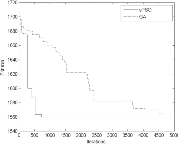
Figure 6 illustrates the convergence of the sPSO method compared with the GA method in 5000 iterations. In addition, the computation time of the sPSO method was approximately the same as the GA method in 5000 iterations. Also, a one-way ANOVA test was conducted to test the hypothesis that µsPSO = µGA for the data of Table 2. The result from the ANOVA test showed that there was a significant difference between the two models since the P-value < 0.001. Hence, based on the comparatively superior performance presented by the sPSO method, we can conclude that our designed sPSO was reliable and consistent in searching for the global optimal or near-optimal solutions.

(20)

15

Table 2

Comparisons from the sPSO Algorithm and the GA method.

GA sPSO sPSO / GA

No.

Instances

Average cost

Lowest cost

Average time(s)

Average cost

Lowest cost

Average time(s)

Average cost IR

Lowest cost IR 1P1 2868.16 2427.59 33.00 1585.80 1585.80 32.42 44.71% 34.68%

2P1 2959.01 2528.13 34.00 1720.70 1720.70 32.52 41.85% 31.94%

3P1 3210.28 2802.07 33.00 1987.80 1987.80 35.59 38.08% 29.06%

4P1 2776.78 2067.09 32.00 1448.20 1448.20 32.37 47.85% 29.94%

5P1 2840.08 2279.37 34.00 1522.50 1522.40 34.34 46.39% 33.21%

6P1 3175.12 2775.93 33.00 1831.40 1831.40 31.26 42.32% 34.03%

7P1 2804.07 2162.07 34.00 1720.50 1714.00 37.47 38.64% 20.72%

8P1 3033.17 2470.61 34.00 1846.60 1833.80 51.27 39.12% 25.78%

9P1 3353.37 2759.57 34.00 2186.70 2159.60 45.96 34.79% 21.74%

10P1 2871.19 2376.62 34.00 1559.50 1559.50 36.70 45.68% 34.38%

11P1 2927.58 2483.71 32.00 1711.70 1711.70 36.34 41.53% 31.08%

12P1 3188.39 2722.65 32.00 2014.80 2014.80 34.05 36.81% 26.00%

13P1 2749.78 2314.38 31.00 1595.10 1593.80 33.20 41.99% 31.13%

14P1 2845.17 2395.29 32.00 1748.70 1748.00 34.80 38.54% 27.02%

15P1 3031.60 2682.36 32.00 2072.20 2032.00 38.39 31.65% 24.25%

16P1 2590.72 1979.30 33.00 1363.80 1363.80 32.41 47.36% 31.10%

17P1 2556.88 2140.13 32.00 1466.30 1466.30 32.44 42.65% 31.49%

18P1 2769.58 2399.18 32.00 1798.40 1798.40 34.54 35.07% 25.04%

19P1 2246.89 1882.65 32.00 1091.90 1088.60 30.89 51.40% 42.18%

20P1 2249.61 1847.61 33.00 1176.60 1176.60 31.10 47.70% 36.32%

21P1 2449.37 2099.34 32.00 1535.70 1535.70 30.83 37.30% 26.85%

22P1 2405.03 1633.10 32.00 1148.80 1148.77 28.77 52.23% 29.66%

23P1 2426.45 1862.76 34.00 1247.20 1247.20 29.09 48.60% 33.05%

24P1 2673.36 2220.77 34.00 1583.70 1583.70 29.07 40.76% 28.69%

25P1 2340.01 1724.51 34.00 1047.40 1047.20 28.79 55.24% 39.28%

26P1 2296.75 1789.07 34.00 1129.70 1129.60 38.04 50.81% 36.86%

27P1 2497.44 2033.66 34.00 1464.70 1464.50 38.29 41.35% 27.99%

28P1 2463.68 1903.41 36.00 1213.50 1213.40 34.30 50.74% 36.25%

29P1 2459.77 1970.18 32.00 1302.10 1302.10 34.09 47.06% 33.91%

30P1 2745.30 2224.62 34.00 1626.80 1626.10 46.77 40.74% 26.90%

31P1 1744.39 1410.99 33.00 1040.80 1040.80 32.81 40.33% 26.24%

32P1 1997.70 1699.74 33.00 1239.80 1239.80 32.31 37.94% 27.06%

(21)

16

Table 2

Comparisons from the sPSO Algorithm and the GA method. (Cont.)

33P1 2868.16 2063.59 33.00 1662.0 1662.80 32.18 42.03% 19.42%

34P1 1643.60 1325.00 34.00 994.39 994.39 30.58 39.50% 24.95%

35P1 1869.79 1527.11 32.00 1194.00 1194.00 30.77 36.14% 21.81%

36P1 2272.05 2008.20 32.00 1606.90 1606.90 32.10 29.28% 19.98%

37P1 1666.12 1390.98 32.00 1119.40 1118.40 33.58 32.81% 19.60%

38P1 1934.95 1634.53 34.00 1286.50 1282.10 38.27 33.51% 21.56%

39P1 2261.51 1968.43 34.00 1668.10 1665.30 38.22 26.24% 15.40%

40P1 1805.12 1464.30 34.00 1064.30 1064.30 30.24 41.04% 27.32%

41P1 1989.66 1636.86 33.00 1254.20 1253.90 30.79 36.96% 23.40%

42P1 2380.18 2004.39 32.00 1668.50 1668.50 29.52 29.90% 16.76%

43P1 1668.72 1349.39 32.00 1135.30 1134.70 28.76 31.97% 15.91%

44P1 1899.70 1519.10 33.00 1334.30 1306.50 29.59 29.76% 14.00%

45P1 2224.75 1979.59 34.00 1684.90 1667.30 69.73 24.27% 15.78%

46P1 2025.59 1681.35 33.00 1146.80 1145.90 34.49 43.38% 31.85%

47P1 2146.87 1753.88 33.00 1327.10 1327.10 36.43 38.18% 24.33%

48P1 2609.74 2185.81 34.00 1712.20 1712.20 35.97 34.39% 21.67%

49P1 1990.00 1473.56 36.00 1375.90 1375.90 30.33 30.86% 6.63%

50P1 2223.77 1761.25 34.00 1284.50 1282.60 44.12 42.24% 27.18%

51P1 2615.53 2073.32 33.00 1744.30 1743.90 31.84 33.31% 15.89%

52P1 2127.57 1677.86 34.00 1303.00 1293.10 41.81 38.76% 22.93%

53P1 2334.54 1709.15 33.00 1460.90 1442.70 52.83 37.42% 15.59%

54P1 2804.30 2329.55 33.00 1835.70 1816.90 39.97 34.54% 22.01%

55P1 2160.84 1852.89 34.00 1222.90 1222.90 30.69 43.41% 34.00%

56P1 2210.49 1912.98 33.00 1429.70 1427.40 29.47 35.32% 25.38%

57P1 2638.74 2251.90 32.00 1861.60 1857.00 35.66 29.45% 17.54%

58P1 2070.97 1740.63 32.00 1223.90 1222.20 36.37 40.90% 29.78%

59P1 2160.69 1859.25 34.00 1401.00 1395.10 40.11 35.16% 24.96%

60P1 2634.82 2368.99 32.00 1847.70 1847.00 32.78 29.87% 22.03%

Avg. I.R. 33.12 35.31 39.30% 26.19%

Std. of I.R Max. I.R Min. I.R

55.24%

24.27%

42.18%

6.63%

(22)

17

Figure 6. Convergence of the sPSO method and the GA method for instance 10P1.

5. Conclusions

In this research, a sPSO algorithm is proposed to approach a combinatorial optimal solution to the vehicle routing problem with Cross-docking system. The primary objectives of this work included the integration of a Cross-docking operation and optimal vehicle routing schedule into a supply chain optimization design. A significant development involves on the synchronization between upstream suppliers and downstream retailers, where both sides of the supply chain are simultaneously considered to collaborate the physical flow of goods in the inbound and outbound processes. With the establishment of this model, the desirable scenario of no customer order delay and no inventory stocking in the central warehouse can be practically achieved.

The computational results show that the sPSO model is effective at solving the VRPCD. The effectiveness of the method comes from the two-phase mechanism. In the initial route-generating phase, a high-quality initial solution is generated by the sweep method before inputting to the routes optimization phase with the particle optimizer functions. The combination of the two phases ensures that the sPSO method yieldd quality solutions.

(23)

18

Sixty benchmark problems were used to investigate the applicability of the proposed particle optimizer. The experimental results showed that the sPSO method is able to produce significant improvements over the GA, surpassing it with an improvement rate of 0.75% for the total average cost generated. In addition, the sPSO method is able to find a better solution than the GA method in 54 instances out of the 60 benchmark problems. Moreover, the sPSO method converges faster to a high quality solution than the GA in 5000 iterations.

REFERENCES

Apte, U.M., Viswanathan S. (2000). Effective cross docking for improving distribution efficiencies. International Journal of Logistics Research and Applications, 3, 291–302.

Bell, J.E., McMullen, P.R. (2004). Ant colony optimization techniques for the vehicle routing problem. Advanced Engineering Informatics, 18(1), 41–48.

Celik, M., Kahraman, C., Cebi, S., Er, I.D. (2009). Fuzzy axiomatic design-based performance evaluation model for docking facilities in shipbuilding industry: The case of Turkish shipyards. Expert Systems With Applications, 36(1), 599–615.

Hu, X., Shi, Y., & Eberhart, R.C. (2004). Recent Advances in Particles Swarm.

Proceedings of IEEE congress on evolutionary computation, 1, 90–97.

Kennedy, J., Eberhart, R.C. (1995). Particle Swarm Optimization, Proc. IEEE International Conference on Neural Networks; IEEE Service Center, Piscataway, NJ, 4, 1942–1948.

LaLonde, B.J., Zinszer, P.H. (1976). Customer Service: Meaning and Measurement.

National Council of Physical Distribution Management, USA.

Lee, Y.H., Jung, J.W., & Lee, K.M. (2006). Vehicle routing scheduling for Cross-docking in the supply chain. Computers & Industrial Engineering, 51(2), 247–256.

Lai, M., Cao E. (2010). An improved differential evolution algorithm for vehicle routing problem with simultaneous pickups and deliveries and time windows.

Engineering Applications of Artificial Intelligence, 23, 188–195.

Marinakis, Y., Marinaki, M. (2010). A hybrid genetic – Particle Swarm Optimization Algorithm for the vehicle routing problem. Expert Systems With Applications, 37(2), 1446–1455.

MirHassani, S.A., Abolghasemi, N. (2011). A particle swarm optimization algorithm for open vehicle routing problem. Expert Systems With Applications, 38(9), 11547–11551.

Mosheiov, G. (1998). Vehicle Routing With Pick-up and Delivery: Tour Partitioning

(24)

19

Heuristics. Computers & Industrial Engineering, 34(3), 669–684.

Rohrer, M. (1995). Simulation and Cross Docking. Proceeding of the 1995 Winter Simulation Conference, 846–849.

Shi, Y., Eberhart, R.C. (1998). A Modified Particle Swarm Optimizer. Proceedings of the IEEE Congress on Evolutionary Computation, 69–73.

Shi, Y., Eberhart, R.C. (1998). Parameter Selection in Particle Swarm Optimization.

1998 Annual Conference on Evolutionary Programming, 591–600.

Song, S.H., Sung, C.S. (2003). Integrated service network design for a Cross-docking supply chain network. Journal of the Operational Research Society, 54, 1283–

1295.

Toth, P., Vigo, D. (2001). The vehicle routing problem. Monographs on Discrete Mathematics and Applications, Philadelphia, PA: SIAM.

Yu W., Egbelu P.J. (2006). Scheduling of inbound and outbound trucks in cross docking system with temporary storage. European Journal of Operational Research, 177, 377–396.

Zachariadis, E.E., Tarantilis, C.D., Kiranoudis, C.T. (2010). An adaptive memory methodology for the vehicle routing problem with simultaneous pick-ups and deliveries. European Journal of Operational Research, 202, 401–411.

改良式粒子群最佳化求解具接駁式轉運之車輛運途問題研究

行政院國家科學委員會專題研究計畫 成果報告