Method for designing a temperature measurement system using two phase-locked loops

(1)

frequency. Then, a single-chip microprocessor is designed to get and compute the duty cycle. Thus, the temperature can be easily computed with the duty cycle, and then sent to a liquid crystal display 共LCD兲 to display. The experimental results show that the resolution of the duty cycle is 1/65280, and the range of the measured temperature is from⫺25.5 to 102 °C with maximum error ⫾0.05 °C in the TMS. Therefore, the main advantages of this system are high resolution, high accuracy, and low cost. © 2003 American Institute of Physics. 关DOI: 10.1063/1.1593814兴

I. INTRODUCTION

Accurate temperature measurements are required in many measurement systems such as process control and in- strumental applications. In most cases, because of the low- level nonlinear effects, the sensor output must be properly conditioned and amplified before further processing.¹ Most of the temperature sensors have a nonlinear transfer function.

In the past, complex analog conditioning circuits were designed to reduce the sensor nonlinearity, manual calibration, and precision resistors were required to achieve the desired accuracy. Today, however, sensor outputs may be digitized directly by high-resolution analog-to-digital 共A/D兲 convert- ers. Linearization and calibration are then performed digi- tally, thereby reducing cost and complexity. Thermocouples can operate over the widest range 共even up to ⫹2300 °C兲 compared with the other temperature sensors. But, their output is only millivolts and precision amplification is required for further processing. Resistance temperature devices 共RTDs兲 are accurate and generally used in bridge circuits, but require excitation current.^2,3 Thermistors have the highest sensitivity but nonlinear problems are also the severest among the three temperature sensors discussed. However, they are popular in portable applications such as measurement of battery temperature and other critical temperatures.⁴ Semiconductor temperature sensors have the characteristics of high accuracy and high linearity over an operating range of about⫺55 to ⫹150 °C. These semiconductor temperature sensors with internal amplifiers can scale the output to either current or voltage values. For example, AD590/TMP17 is a current output sensor with scale factors of 1 ␮^{A/K, and} TMP35/TMP36/TMP37 are low voltage output sensors with a 10/20 mV/°C scale factor.⁵ However, their outputs require precision amplification for further processing. The digital

temperature sensors such as the TMP03/TMP04/SMT160 with digital outputs have a number of advantages over those with analog outputs, especially in remote application. The popular microcontrollers, such as the MSC-51 and 68xx11 series, have on-chip timers, which can easily decode the mark-space ratio of the digital temperature sensors. The SMT160 is basically a bipolar temperature sensor, with accurate electronics to convert the sensor signal into a duty cycle,⁶ and it can connect to all kinds of microcontrollers directly with one wire 共duty cycle兲 output without any A/D conversion. Since the duty cycle of the output signal is linearly related to the temperature, the temperature can be easily computed by means of measuring a duty cycle.

The traditional method to measure the duty cycle signal is to use a clock to count the signal.⁷An error will be generated due to the asynchronous timing. For example, in Fig.

1 the timing errors between the clock edge and the signal edge are E1, E2, and E3. The one drawback of this method is the need for an ultra-high-frequency counter clock in order to achieve high resolution and high accuracy. For example, a 4 kHz input signal to get 1/60 000 resolution will require a 240 MHz counter clock. Therefore, practical application of this traditional method is limited by the high frequency of the digital circuitry.

An ‘‘accumulated’’ type of computing duty cycle, modified from the traditional method shown in Fig. 2, is designed to accumulate the counts in m periods to improve the accuracy.⁸ For m times improvement of accuracy, it has to waste m signal periods to wait for only one average duty cycle, thus limiting the output rate.

In this article, a method is developed to achieve accurate duty cycle measurements and to obtain high-precision temperature measurements. Basically, the proposed technique is based on the phase-locked-loop PLL circuit to emulate a Ver- nier caliper.^9–11 One PLL emulates the main scale of the Vernier caliper, and the other is a movable Vernier scale. A

a兲Author to whom correspondence should be addressed; electronic mail:

msyoung@mail.ncku.edu.tw

3826

(2)

coarse measurement is done by the main scale, and then a fine measurement is adopted to refine the final result by the Vernier scale. Thus, high accuracy and high resolution is achieved.

II. METHOD

A Vernier caliper is composed of two scales, the main scale and the movable Vernier scale as shown in Fig. 3. The unit lengths L 共L usually equals the length of Vernier scale兲 are divided into equal segments of physical length by in- scribing lines into the metal of the caliper scales. If unit length L on the main scale is divided into M divisions and on the Vernier scale into N divisions 共where M⫽cN⫺1, c is positive integer, and in Fig. 3, c⫽2), it can be found that the smallest physical length measurable with the caliper is L/( M*N)⫽L/关(cN⫺1)*N兴 long. Transforming from a physical distance to temporal length of wave period degrees, the new method sets unit length L equal to the wave period of the input signal, and the caliper divisions are replaced

with equal time slots within the period. Cutting the periods into multiple equal time slots can be implemented by using PLL circuit. A Vernier caliper emulator 共VCE兲 circuit as shown in Fig. 4 is carefully designed to emulate the Vernier caliper. With a real caliper, the user may measure a physical length less or more than the unit length L, while with the VCE, the measured duty cycle is always less than 1. Two frequency multiplying PLL circuits generate two clocks in the VCE, which function as the dividing lines inscribed two temporal scales, one clock for the main scale and the other for the Vernier scale.

If the unit length L on the both scales is divided into M 共on the main scale兲 and N 共on the Vernier scale兲 divisions, a given measured length X can be represented as

X⫽p⫹L

冉

^M^m^⫹^Mⁿ^*^N^⫹^M^e^*^N

冊

^, ^共1兲

where M⫽cN⫺1, 0⭐p, 0⭐m⭐M, 0⭐n⭐N, 0⭐e⭐1.

In Eq.共1兲, p, m, and n are all integers, and e is a real number. On a mechanical Vernier caliper, the value p repre- sents the integer part of the real measured length out of the unit length L. The value of m and n are read from the main scale and the Vernier scale. The resolution of the Vernier caliper is L/( M*N), the value e is the residual part of the length X that is less than the resolution of the Vernier caliper, and so the term of L*(e/ M*N) can be eliminated. The Eq.

共1兲 can be modified as

X⫽p⫹L

冉

^M^m^⫹^Mⁿ^*^N

冊

^. ^共2兲

The principle of the VCE inherits the Vernier caliper’s fundamental concept. In the VCE, L is set to a period of input signal, the duty cycle is less than 1, and the value p is zero. Thus, the measurement result of a duty cycle can be expressed as Eq.共3兲:

DC⫽T1 T2⫽m

M⫹ n

M*N, 共3兲

FIG. 1. Traditional method using a clock to measure the duty cycle.

FIG. 2. Accumulated method was to accumulate the counts in m periods to improve the accuracy.

FIG. 3. Vernier caliper: the measured length X⫽39*关15/39⫹16/(39*_20)兴

⫽15.8 mm is read out with resolution 0.05 mm, unit length of L⫽39 mm, M⫽39, N⫽20, p⫽0, m⫽15, and n⫽16.

Downloaded 24 Oct 2008 to 140.116.208.51. Redistribution subject to AIP license or copyright; see http://rsi.aip.org/rsi/copyright.jsp

(3)

where DC is duty cycle, T1 is the length of ‘‘1’’ of signal, T2 is the period of signal.

III. SYSTEM IMPLEMENTATION

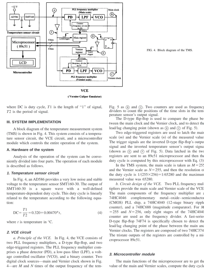
A block diagram of the temperature measurement system 共TMS兲 is shown in Fig. 4. This system consists of a temperature sensor circuit, the VCE circuit, and a microcontroller module which controls the entire operation of the system.

A. Hardware of the system

Analysis of the operation of the system can be conveniently divided into four parts. The operation of each module is described as follows.

1. Temperature sensor circuit

In Fig. 4, an AD586 provides a very low noise and stable voltage to the temperature sensor SMT160-30. The output of SMT160-30 is a square wave with a well-defined temperature-dependent duty cycle. This duty cycle is linearly related to the temperature according to the following equation:

DC⫽T1

T2⫽0.320⫹0.00470*t, 共4兲

where t is temperature in °C.

2. VCE circuit

a. Principle of the VCE. In Fig. 4, the VCE consists of two PLL frequency multipliers, a D-type flip-flop, and two edge-triggered registers. The PLL frequency multiplier com- prises a phase detector共PD兲, a low-pass filter 共LPF兲, a voltage controlled oscillator 共VCO兲, and a binary counter. Two digital clock sources—main and Vernier clock shown in Fig.

4—are M and N times of the output frequency of the tem- perature sensor. For convenience, the constant c关c⫽(M

⫹1)/N兴 is selected as 1. The timing diagrams are shown in

Fig. 5 as ^B and ^C. Two counters are used as frequency dividers to count the positions of the time slots in the temperature sensor’s output signal.

The D-type flip-flop is used to compare the phase between the main clock and the Vernier clock, and to detect the lead/lag changing point共shown as ^B and C of Fig. 5兲.

Two edge-triggered registers are used to latch the main scale 共m兲 and the Vernier scale 共n兲 of the measured value.

The trigger signals are the inverted D-type flip-flop’s output signal and the inverted temperature sensor’s output signal 共shown as ^E and F of Fig. 5兲. Data latched in the two registers are sent to an 89c51 microprocessor and then the duty cycle is computed by this microprocessor with Eq.共3兲.

In the TMS system, the main scale is taken as M⫽255 and the Vernier scale as N⫽255, and then the resolution of the duty cycle is 1/共255⫻256兲⫽1/65280 and the maximum measured value was 65280.

b. Circuit design of the VCE. Two PLL frequency mul- tipliers provide the main scale and Vernier scale of the VCE.

The main components of the frequency multiplier are a 74HC4046 complementary metal–oxide–semiconductor 共CMOS兲 PLL ship, a 74HC4040 共12-stage binary ripple counter兲, and a 74HC688 共magnitude comparator兲. For M

⫽255 and N⫽256, only eight stages of the 74HC4040 counter are used as the frequency divider. A fast-series D-type flip-flop 74F74 is specifically chosen to detect the lead/lag changing point of the phase between the main and Vernier clocks. The registers are composed of two 74HC374.

The tristate outputs of the registers are controlled by a microprocessor 89c51.

3. Microcontroller module

The main functions of the microprocessor are to get the value of the main and Vernier scales, compute the duty cycle and the target temperature, and then send the temperature to a LCD to display.

(4)

4. Calibration system

The calibration of the TMS can be conveniently divided into two parts and described as follows:

共a兲 Calibrating the VCE: The VCE must be calibrated by a calibration signal with a known duty cycle and frequency. The calibration signal is generated from a function generator 共HP 33120A function generator/

arbitrary wave-form generator兲, which can output a signal with the range of the duty cycle from 20% to 80%.

共b兲 Calibrating the TMS system: A known temperature verified by the National Instrument NI 4350 temperature measurement system was used to calibrate the TMS in a temperature-controlled chamber.

B. Software of the system

Software for the 89c51 microprocessor is programed in C language共IAR兲 and described by the flow chart in Fig. 6.

The main program will check the interrupt flag of the VCE to get the main and Vernier scales, calculate the duty cycle, and display the temperature on the LCD. The system will be restart when the Watchdog timer indicates an overflow to avoid a system crash.

IV. TESTING THE SYSTEM

A prototype TMS with no temperature sensor was tested to check the accuracy and linearity of the VCE. The frequencies of the test signals that replaced the outputs of temperature sensor were selected as 1, 2, 3, and 4 kHz, since the frequency of the temperature sensor output signal was within the range from 1 to 4 kHz. The HP 33120A function generator can only output a signal with the range of the duty cycle from 20% up to 80% and with 1% minimum increment, thus the test signal’s duty cycle was controlled to increase 1%

each time within this range.

Logged data graphs of the measured duty cycle versus actual duty cycle are shown in Figs. 7共a兲, 8共a兲, 9共a兲, and 10共a兲. The error data were the difference between the actual duty cycle and the measured duty cycle shown in Figs. 7共b兲, 8共b兲, 9共b兲, and 10共b兲, and the error range was within ⫺5–20.

The percentage errors共PEs兲 of the measured duty cycle were calculated by the following equation:

PE⫽兺ⁿ_i

冏

^{R P}^{共i兲⫺PP共i兲}^{P P}共i兲

冏

n ⫻100%, 共5兲

where R P is the measured duty cycle, P P is the actual duty

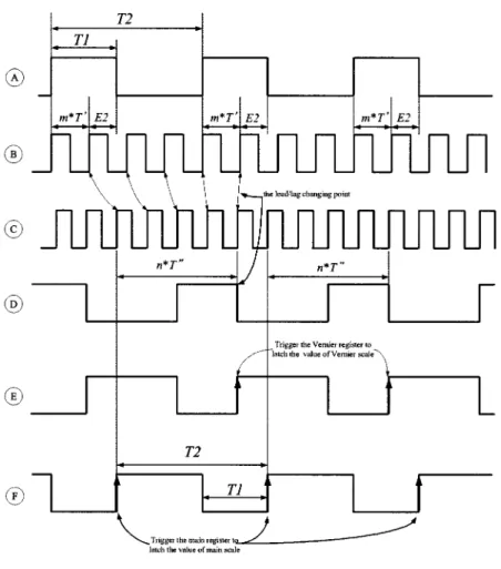
FIG. 5. 共a兲 Wave of Â is the temperature sensor’s output.共b兲 Wave of ^B is the main clock.共c兲 Wave of ^C is the Vernier clock.共d兲 Wave of ^D is the D-type flip- flop’s output.共e兲 Wave of Ê is the inverted D-type flip-flop’s output.共f兲 Wave of ^F is the inverted temperature sensor’s output. Measured duty cycle of Â is DC⫽T1/T2⫽1/4⫹4/(4*5)⫽9/20 with resolution 1/20, M⫽4, N⫽5, m⫽1, and n⫽4.

(5)

cycle of the input signal, and n is the number of measured data. The frequencies 1, 2, 3, and 4 kHz of the PE were 0.0189%, 0.0176%, 0.0186%, and 0.0196%.

In Figs. 7共b兲, 8共b兲, 9共b兲, and 10共b兲, the peak errors oc- curred periodically. Owing to this phenomenon a software program was designed as a digital filter to reduce these peak errors. The software program was designed to get and sort the measured data around the peak error, and calculate the mean of the sorted data between the value of PR₂₅ 共percent- age rank兲 to PR75 to erase the peak error. Thus, the error

FIG. 6. Software flow chart of the system.

FIG. 7. 共a兲 Logged data graph of the actual duty cycle vs measured duty

FIG. 8. 共a兲 Logged data graph of the actual duty cycle vs measured duty cycle at f⫽2 kHz. 共b兲 Error plot of the measured duty cycle.

FIG. 9. 共a兲 Logged data graph of the actual duty cycle vs measured duty cycle at f⫽3 kHz. 共b兲 Error plot of the measured duty cycle.

FIG. 10. 共a兲 Logged data graph of the actual duty cycle vs measured duty

(6)

range would reduce to⫺5–12, and the precision rate would increase to 99.931%.

V. EXPERIMENTAL RESULTS

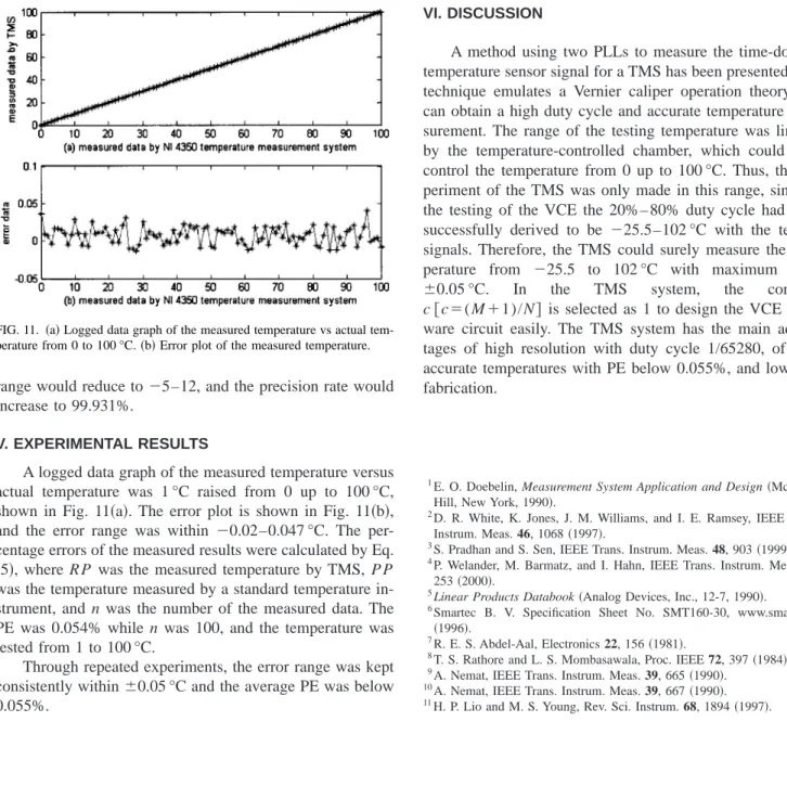
A logged data graph of the measured temperature versus actual temperature was 1 °C raised from 0 up to 100 °C, shown in Fig. 11共a兲. The error plot is shown in Fig. 11共b兲, and the error range was within ⫺0.02–0.047 °C. The percentage errors of the measured results were calculated by Eq.

共5兲, where RP was the measured temperature by TMS, PP was the temperature measured by a standard temperature in- strument, and n was the number of the measured data. The PE was 0.054% while n was 100, and the temperature was tested from 1 to 100 °C.

Through repeated experiments, the error range was kept consistently within⫾0.05 °C and the average PE was below 0.055%.

periment of the TMS was only made in this range, since in the testing of the VCE the 20%– 80% duty cycle had been successfully derived to be ⫺25.5–102 °C with the testing signals. Therefore, the TMS could surely measure the temperature from ⫺25.5 to 102 °C with maximum error

⫾0.05 °C. In the TMS system, the constant c关c⫽(M⫹1)/N兴 is selected as 1 to design the VCE hardware circuit easily. The TMS system has the main advantages of high resolution with duty cycle 1/65280, of high accurate temperatures with PE below 0.055%, and low cost fabrication.

1E. O. Doebelin, Measurement System Application and Design共McGraw- Hill, New York, 1990兲.

2D. R. White, K. Jones, J. M. Williams, and I. E. Ramsey, IEEE Trans.

Instrum. Meas. 46, 1068共1997兲.

3S. Pradhan and S. Sen, IEEE Trans. Instrum. Meas. 48, 903共1999兲.

4P. Welander, M. Barmatz, and I. Hahn, IEEE Trans. Instrum. Meas. 49, 253共2000兲.

5Linear Products Databook共Analog Devices, Inc., 12-7, 1990兲.

6Smartec B. V. Specification Sheet No. SMT160-30, www.smartec.nl 共1996兲.

7R. E. S. Abdel-Aal, Electronics 22, 156共1981兲.

8T. S. Rathore and L. S. Mombasawala, Proc. IEEE 72, 397共1984兲.

9A. Nemat, IEEE Trans. Instrum. Meas. 39, 665共1990兲.

10A. Nemat, IEEE Trans. Instrum. Meas. 39, 667共1990兲.

11H. P. Lio and M. S. Young, Rev. Sci. Instrum. 68, 1894共1997兲.