平板與翼剖面之紊流和過渡之分析

※※※※※※※※※※※※※※※※※※※※※※※※※※※※※※※※※※※※※

※ ※

※ 平板與翼剖面之紊流和過渡之分析 ※

※

※ Flow Over Flat Plate and Air foil

※ ※

※※※※※※※※※※※※※※※※※※※※※※※※※※※※※※※※※※※※※

計劃編號：NSC 90-2212-E-006-147

執行期間：90 年 8 月 1 日至 91 年 7 月 31 日 計劃主持人：林三益 成功大學航太所教授 助理研究員：黃百毅 成功大學航太所研究生

一、中文摘要

本文的目的是調整並結合三個低雷諾數雙 方 程 式 ： Jones-Launder，Launder-Sharma 和 Chien 的紊流模式中的常數與震盪函 數。調整方法是根據這些紊流模式的過渡 流場區域的位置，加以分析調整。調整後 的計算結果與平板的實驗值比較。比對的

物理參數有表面摩擦係數(

C

子(

H

R e

(

u

正模式最理想的是不需要在紊流模式中使 用過渡流場的起始點與流場長度的經驗公 式，而能準確的預測過渡流場的起始點與 流場長度。其中也探討了層流流場擾動量 與實驗值的差異，發現是紊流標準模式無 法準確估計在層流中帶有擾動的流場，但 在過渡流和紊流流場，修正的紊流模式能 夠準確估計其物理量和流場特性。

英文摘要

A modified low-Reynolds-number k−ε model is proposed for calculations of bypass transitional boundary-layer flows. This modified model is combining the Jones- Launder, Launder-Sharma, and Chien k−ε models by adjusting their model constants and damping functions. The computations are performed by a compressible Navier- Stokes solver which solved the mean flow and the modified bypass-transition low- Reynods-number k−ε turbulence equations.

The solver used a third-order upwind finite- volume method for the convection terms, a

second-order central finite-volume method for the viscous terms, and a three-step Runge-Kutta method for the time marching.

Calculations are carried for transitional boundary-layer flows over a flat plate under various free-stream turbulence levels. The computational results show that the profiles of mean velocity and turbulent intensity, the distributions of skin friction and shape functions are well predicted. The transition onset and length are also compared well with the experimental data.

2. INTRODUCTION

The mechanism of transition from laminar to turbulent flow remains one of very important research subjects in fluid dynamics. Since the increase of skin friction and heat transfer in the transition flows, the ability to predict the transition region is important in many industrial applications.

However, no mathematical model exists which can accurately predict the location of transition for most of real application flows.

Bypass transition occurs under the influence of free-stream turbulence.¹ This is different to the natural transition, which usually occurs under the Tollmien-Schlichting instability wave. Savil assembled a series of experimental test cases: T3A, T3AM, and T3B.² The experiments were selected to test the abilities of turbulence models to predict the location of transition under the influence of free-stream turbulence.

Concerning with the numerical methods for computing transition flows, the eⁿ method is a traditional method to determine the onset of transition. Unfortunately, the value of n is not constant and is related the external disturbance environment. Also, the method may not be useful for predicting the bypass transition. Savil has reviewed most of the existing two-equation turbulence models for the prediction of the bypass transition and concluded that, compared with the measurements, the predicted transition onsets were mostly too early and the length of transition region were too short. Different attempts to improve the ability of two- equation turbulence models on the transition prediction have been suggested. The use of the correlation of the transition onset to determine the transition point and the introduce of the intermittency parameter to determine the transition length were the two common ways for most bypass transition models. Abu-Ghannam and Shaw,³ Gostelow et. al.,⁴ Mayle,¹ and Suzen et. al.⁵ gave some correlations for the transition onset. Some researchers also used different correlations for the intermittency parameter.

On the other way, some authors proposed a separate transport equation for the intermittency parameter. In this paper, a modified low-Reynolds-number k−ε model is proposed. The model is combining the Jones-Launder, Launder-Sharma, and Chien models by adjusting their model constants and damping functions.^6-8 By this way, the intermittency parameter for the transition length and the correlation for the transition onset are not necessary in this model.

In the following sections, the details of the modified two-equation turbulence models and the correlations of the transition onset and length are given. The boundary condition procedures are also included. Then, calculations are performed for bypass transition boundary-layer flows over a flat plate under various freestream turbulence levels. The numerical results show good agreements with the experimental data.

3. NUMERICAL FORMULATIONS

3.1 Gover ning Equations:

A low-Reynolds-number k−ε model can be written as

2

1 1 2 2

2

[( ) ]

[( ) ]

{ [ ] 2 3 2 3 }

j

t k k k

j j j

j

t k

j j j

i i j k i

k ij T T ij ij

j j i k j

t

k ku k

P L

t x x x

u c f P c f L

t x x x k k

u u u u u

P k

x x x x x

c f k

ε ε

µ µ

ρ ρ µ µ σ ρε

ρε ρε µ µ σ ε ε ρε

τ µ µ δ ρ δ

µ ρ ε

∂ +∂ − ∂ + ∂ = − −

∂ ∂ ∂ ∂

∂ +∂ − ∂ + ∂ = − +

∂ ∂ ∂ ∂

∂ ∂ ∂ ∂ ∂

= ′ = + − −

∂ ∂ ∂ ∂ ∂

=

Here (L L_k, _ε) are the low-Relynolds-number terms. σ_k , σ_ε , c_µ , c , ₁ c are the model ₂ constants and f_µ , f , ₁ f are the damping ₂ functions. These parameters depend on the turbulence model chosen. Based on the effects of these parameters⁹, the modified k−ε model is then proposed and related parameters are followings:

1 2

1.7

1

2

2

2

2 2

2

0.09 1.44 1.95 1. 1.3

exp[ 3.11 (1. 0.02 Re ) ] 1.

1. 0.22 exp( Re ) 36.

2 ( )

2 ( )

Re /

k

T

T

k

j

i T

j l

T

c c c

f f f L k

x L u

x x k

µ ε

µ

ε

σ σ

µ µµ

ρ

ρ εµ

= = = = =

= − +

=

= − −

= ∂

∂

= ∂

∂ ∂

=

3.2 Numer ical Method and Boundar y Conditions:

The computations are performed by a compressible Navier-Stokes solver which solve the mean flow and bypass-transition low-Reynods-number k−ε turbulence equations. The method used a third-order upwind finite-volume method for the convection terms, a second-order central

finite-volume method for the viscous terms, and a three-step Runge-Kutta method for time marching. The freestream Mach number is chosen as 0.2, so that that the flow can be seen to be incompressible. The grid independence and the effect of Mach number were investigated in the paper.⁹

The leading edge of the flat plate is at x=0 and the inlet position of the computational domain is at x= −l₀ . The boundary conditions for k and ε at the inlet is determined by the freestream turbulence intensity and the the decay of the freestream turbulence which are obtained from the experimental data. For the given k_∞ at the inlet, the value of ε_∞ is then determined to agree with the experimental data.

4. RESULTSAND DISCUSSIONS

The modified model is used to predict the bypass transition of the experimental test cases assembled by Savill: T3A, T3AM, and T3B.²

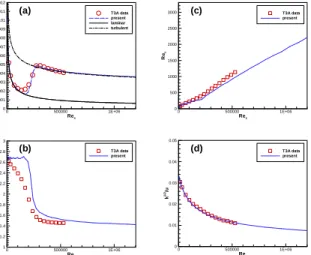
4.1 T3A case:

T3A experiment corresponds to a zero- pressure-gradient flow over a flat plate at

105

6 . 3

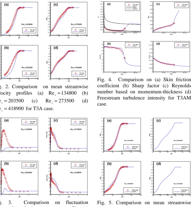
Re= × per meter. The upstream turbulence intensity at the inlet of the flat plate is 3 percent. The comparison results obtained by the modified model are shown in Figures 1, 2, and 3. The model can compute the skin friction very well in whole flow range as shown in Figure 1 (a). The transition onset and the transition length conform to the experiment data. Only the transition onset is a very slightly delay. The freesteam turbulence intensity, sharp factor, and Re_θ number are compared well to the experiment data as shown in Figures 1 (b), (c), and (d), respectively. Figure 2 shows the comparisons of the streamwise mean velocity profiles at the four positions in the transition region. The results agree well with the experimental data except some discrepancy at Re_x=203500 . The streamwise velocity fluctuation, u , at the ^' four positions are shown in Figure 3. The positions in Figures 3 (a) and (b) are located in the laminar region. Although the model

can’t capture well in the “pretransition”

region, it can capture the streamwise velocity fluctuation well in the region after the transition onset as Figures 3 (c) and (d) shown.

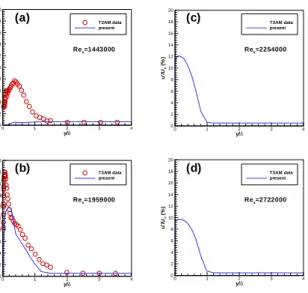
4.2 T3AM Case:

T3AM experiment corresponds to a zero-pressure-gradient flow over a flat plate at Re=13.2 10× ⁵ per meter. The upstream turbulence intensity at the inlet of the flat plate is 1 percent. The skin friction is estimated very well in whole flow range as shown in Figure 4 (a). The transition onset and the transition length conform to the experiment data. The freesteam turbulence intensity, sharp factor, and Re_θ number are compared well to the experiment data as shown in Figures 4 (b), (c), and (d), respectively. Figure 5 shows the comparisons of the streamwise mean velocity profiles at the four positions in the transition region. The results agree well with the experimental data at Re_x=1443000 and Re_x =1959000 . There is no experimental data after Re_x=2021600. The streamwise velocity fluctuation, u , at the four positions ^' are shown in Figure 6. The position in Figure 6 (a) is located in the laminar region. Again the model can’t capture well in the

“pretransition” region. After the middle point of the transition region, Figures 6 (b) and (c) show the streamwise velocity fluctuation of the modified model. Figure 6 (d) is located in the fully turbulent region.

4.3 T3B Case:

The final test case is the T3B case. It corresponds to a zero-pressure-gradient flow over a flat plate at Re=6.3×10⁵ per meter.

The upstream turbulence intensity at the inlet of the flat plate is 6 percent. The computational results are also compared well with the experimental data.

5. CONCLUSIONS

The modified k−ε model is developing for calculations of bypass transitional boundary-layer flows. By only

adjusting the model constant c and the ₂ damping functions f_µ and f in a standard ₂ low-Reynolds-number k−ε turbulence model, a modified low-Reynolds-number k−ε model is then formatted. It doesn’t use the correlations for the transition onset and the intermittent factor as most bypass transition model used. That is the modified model belongs to the standard low- Reynolds-number k−ε model and can well predict the transition onset and length in the bypass transition flow over a flat plate under several freestream turbulence intensity levels.

The modified model is used to simulate the T3A, T3AM, and T3B experiments.

Comparisons of the skin friction distributions and the developed boundary layers are matched for all cases. The results show that the modified model can predict the bypass transition well.

ACKNOWLEDGEMENTS

This work was partially supported by the National Science Council of the Republic of China under Contract NSC90-2212-E- 006-147. The authors also thank P. G. Huang for providing the T3A, T3AM, and T3B experimental data.

REFERENCES

1. Mayle, R. E., 1991, “The Role of Laminar-Turbulent Transition in Gas Turbine Engines,” ASME J. Turbomach., 113, pp. 509-537.

2. Savill, A. M., 1993, “Further Progress in The Turbulence Modeling of Bypass Transition,” Engineering Turbulence Modeling and Experiments 2, W. Rodi and F. Martelli, eds., Elsevier Science, pp.

583-592.

3. Abu-Ghannam, B. J. and Shaw, R. 1980,

“Natural Transition of Boundary Layers- The Effects of Turbulence, Pressure Gradient, and Flow History,” Journal of Mechanics Engineering Science, 22, No. 5, pp. 213-228.

4. Gostelow, J. P., Blunden, A. R., and Walker, G. J., 1994, “Effects of Freestream Turbulence and Adverse

Pressure Gradients on Boundary Layer Transition,” ASME J. Turbomach., 116, pp. 392-440.

5. Suzen, Y.B. and Huang, P.G., 2000,

"Modeling of Flow Transition Using an Intermittency Transport Equation,"

Journal of Fluids Engineering, 122, 273- 284.

6. Jones, W. P. and Launder, B. E., 1973,

“The Calculation of Low-Reynolds- Number Phenomena with a Two-Equation Model of Turbulence,” Int. J. Heat Mass Transfer, 16, pp. 1119-1130.

7. Launder, B. E. and Sharma, B. I., 1974,

“Application of the Energy-Dissipation Model of Turbulence to The calculation of Flow Near a Spinning Disc,” Letters in Heat and Mass Transfer, 1, pp. 131-139.

8. Chien, K. Y. 1982, “Predictions of Channel and Boundary-Layer Flows with a Low-Reynolds-Number Turbulence Model,” AIAA Journal, 82-0020.

9. Hwang, B. Y., 2001, “Two-Equation Turbulence Models for Transition Flow Over a Flat Plate,” Institute of Aeronautics and Astronautics, National Cheng Kung University, Dissertation for Doctor of Philosophy.

Rex H=δ*/θ

0 500000 1E+06

1 1.2 1.4 1.6 1.8 2 2.2 2.4 2.6 2.8 3

T3A data present

(b)

Rex Reθ

0 500000 1E+06

0 500 1000 1500 2000 2500

3000 T3A data

present

(c)

Rex k1/2/u

0 500000 1E+06

0 0.01 0.02 0.03 0.04 0.05

T3A data present

(d)

Rex Cf

0 500000 1E+06

0 0.001 0.002 0.003 0.004 0.005 0.006 0.007 0.008 0.009 0.01 0.011 0.012

T3A data present laminar turbulent

(a)

Fig. 1. Comparison on (a) Skin friction coefficient (b) Sharp factor (c) Reynolds number based on momentum-thickness (d) Freestream turbulence intensity for T3A case.

y/δ u/Ue

10^-2 10^-1 10⁰ 10¹ 10²

0 0.1 0.2 0.3 0.4 0.5 0.6 0.7 0.8 0.9 1 1.1 1.2

T3A data present Re_x=134800

(a)

y/δ u/Ue

10^-2 10^-1 10⁰ 10¹ 10²

0 0.1 0.2 0.3 0.4 0.5 0.6 0.7 0.8 0.9 1 1.1 1.2

T3A data present Re_x=273500

(c)

y/δ u/Ue

10^-2 10^-1 10⁰ 10¹ 10²

0 0.1 0.2 0.3 0.4 0.5 0.6 0.7 0.8 0.9 1 1.1 1.2

T3A data present Rex=418900

(d)

y/δ u/Ue

10^-2 10^-1 10⁰ 10¹ 10²

0 0.1 0.2 0.3 0.4 0.5 0.6 0.7 0.8 0.9 1 1.1 1.2

T3A data present Rex=203500

(b)

Fig. 2. Comparison on mean streamwise velocity profiles (a) Re_x=134800 (b) Re_x=203500 (c) Re_x =273500 (d) Re_x=418900 for T3A case.

y/δ u'/Ue(%)

0 1 2 3 4

0 2 4 6 8 10 12 14 16 18 20

T3A data present

Re_x=134800

(a)

y/δ u'/Ue(%)

0 1 2 3 4

0 2 4 6 8 10 12 14 16 18 20

T3A data present

Re_x=273500

(c)

y/δ u'/Ue(%)

0 1 2 3 4

0 2 4 6 8 10 12 14 16 18 20

T3A data present

Re_x=418900

(d)

y/δ u'/Ue(%)

0 1 2 3 4

0 2 4 6 8 10 12 14 16 18 20

T3A data present

Re_x=203500

(b)

Fig. 3. Comparison on fluctuation streamwise velocity component profiles (a) Re_x=134800 (b) Re_x=203500 (c) Re_x=273500 (d) Re_x =418900 for T3A case.

Rex Reθ

0 1E+06 2E+06 3E+06

0 500 1000 1500 2000 2500 3000 3500 4000

T3A1 data present

(c)

Rex Cf

0 1E+06 2E+06 3E+06

0 0.001 0.002 0.003 0.004 0.005 0.006 0.007 0.008 0.009 0.01 0.011 0.012

T3A1 data present laminar turbulent

(a)

Rex H=δ*/θ

0 1E+06 2E+06 3E+06

1 1.2 1.4 1.6 1.8 2 2.2 2.4 2.6 2.8 3

T3A1 data present

(b)

Rex k1/2/u

0 1E+06 2E+06 3E+06

0 0.0025 0.005 0.0075 0.01 0.0125 0.015 0.0175 0.02

T3A1 data present

(d)

Fig. 4. Comparison on (a) Skin friction coefficient (b) Sharp factor (c) Reynolds number based on momentum-thickness (d) Freestream turbulence intensity for T3AM case.

y/δ u/Ue

10^-2 10^-1 10⁰ 10¹ 10²

0 0.1 0.2 0.3 0.4 0.5 0.6 0.7 0.8 0.9 1 1.1 1.2

T3AM data present Re_x=1443000

(a)

y/δ u/Ue

10^-2 10^-1 10⁰ 10¹ 10²

0 0.1 0.2 0.3 0.4 0.5 0.6 0.7 0.8 0.9 1 1.1 1.2

T3AM data present Re_x=1959000

(b)

y/δ u/Ue

10^-3 10^-2 10^-1 10⁰ 10¹ 10²

0 0.1 0.2 0.3 0.4 0.5 0.6 0.7 0.8 0.9 1 1.1

T3AM data present Re_x=2254000

(c)

y/δ u/Ue

10^-3 10^-2 10^-1 10⁰ 10¹ 10²

0 0.1 0.2 0.3 0.4 0.5 0.6 0.7 0.8 0.9 1 1.1 1.2

T3AM data present Re_x=2722000

(d)

Fig. 5. Comparison on mean streamwise velocity profiles (a) Re_x=1443000 (b) Re_x=1959000 (c) Re_x=2254000 (d) Re_x=2722000 for T3AM case.

y/δ u'/Ue(%)

0 1 2 3 4

0 2 4 6 8 10 12 14 16 18 20

T3AM data present

Rex=1443000

(a)

y/δ u'/Ue(%)

0 1 2 3 4

0 2 4 6 8 10 12 14 16 18 20

T3AM data present

Re_x=1959000

(b)

y/δ u'/Ue(%)

0 1 2 3 4

0 2 4 6 8 10 12 14 16 18 20

T3AM data present

Rex=2254000

(c)

y/δ u'/Ue(%)

0 1 2 3 4

0 2 4 6 8 10 12 14 16 18 20

T3AM data present

Re_x=2722000

(d)

Fig. 6. Comparison on fluctuation streamwise velocity component profiles (a) Re_x=1443000 (b) Re_x=1959000 (c) Re_x=2254000 (d) Re_x=2722000 for T3AM case.