出血性大腸桿菌之建模與模擬驗證

全文

(1)國立成功大學航空太空工程學系碩士論文. 出血性大腸桿菌之建模與模擬驗證 Kinetics modeling and simulation verification of Escherichia coli O157:H7. 研究生：洪紹展. Student: Shao-Jhan Hong. 指導教授：楊憲東. Advisor: Ciann-Dong Yang. 中華民國一 O 二年六月.

(2)

(3) 中文摘要. 近年研究中，對於細胞中主要代謝途徑如醣酵解作用(glycolysis)、檸檬酸循環(tricarboxylic acid cycle)、五碳醣磷酸(pentose phosphate)以及回補途徑(anapleorotic pathway)等建立了數學模型，用以模擬代謝物反應的行為。而這些理論更被用在結核桿菌(Mycobacterium tuberculosis)、盤基網柄菌(Dictyostelium discoideum)、釀酒酵母(Saccharomyces cerevisiae)和大腸桿菌 (Escherichia coli)上面進行不同的用途。從生化實驗中得知，出血性大腸桿菌(E. coli O157:H7)中檸檬酸循環過程的琥珀酸去氫酶(succinate dehydrogenase)做一突變時，其代謝物反應濃度會有顯著的差異。本論文中我們將針對出血性大腸桿菌提出相對應之數學模型，並基於 Matlab 在控制、數值領域應用上的便利性建立其模擬環境，如此可以透過數值模擬各代謝物濃度變化來比對實驗數據，驗證模組的可行性，另外使用此模組來預測其他酵素突變的關係。在此所提出的相關參數、模型以及實驗數據實際上都是以體外環境 (vivo environment)做討論。. 關鍵字：大腸桿菌、生物化學、酵素動力學、代謝途徑. i.

(4) ABSTRACT. In the recent years, many efforts have been given to simulate the dynamic behavior of metabolism of a cell using mathematical models for the main metabolic pathways such as glycolysis, tricarboxylic acid cycle (TCA cycle), pentose phosphate (PP) pathway, and the anapleorotic pathways, etc. These models have been applied to the Mycobacterium tuberculosis, Dictyostelium discoideum, Saccharomyces cerevisiae and Escherichia (E.) coli for different verification purposes. The significant change of metabolite concentrations as knockout of succinate dehydrogenase on metabolism in TCA cycle of E. coli O157:H7 has been observed from experiments in biochemistry. Here we construct a mathematical model to describe this observation by using the simulation environment of Matlab. A least-square iterative scheme is proposed to tune the kinetic parameters in the model so as to minimize the matching error between the output of the model and the experimental data. The metabolite concentrations computed by the model are compared with the experimental data to verify the feasibility of the proposed model. Based on the same model, we also reveal predictions on new mutants, which are to be confirmed by experiments.. Keywords: Escherichia coli, biochemical, enzyme kinetics, metabolic pathway. ii.

(5) 誌謝. 本論文能夠順利完成，首要感謝楊憲東老師在我碩班生涯中，指導我做研究的方法以及態度，並且提供建議修改碩士論文，使得各章節論述更加順暢；老師的研究精神更成為我努力學習的典範，不僅在研究上的造詣，處世的態度也讓我更懂得做人，這是我成長最多的地方。同時感謝碩士論文口試委員吳煒老師和陳昌熙老師，在跨領域的合作中，學習了寶貴的經驗，以及兩位老師在口試期間給予的鼓勵和建議，補足了非自身領域所欠缺的知識。感謝冠璋學長，在研究所中讓我的程式應用更加精進，使得我論文中程式的撰寫更加順利；感謝登驛學長、旻琦學長和烈烈學長，給予鼓勵與支持，適度參與討論和建議，才讓我找到更多方式；感謝同窗的林育和仲軒，一起走過精彩的兩年碩班生活，彼此互相鼓勵與支持也是動力來源之一。感謝研究室的學弟們：柯宗良、黃仁顥和林祖瑋在口試期間的協助，謝謝你們。感謝最親愛的爸爸、媽媽和老哥，在背後給我最大的支持，讓我無慮專心完成研究，今日能夠成長至此，最大功勞是不辭辛勞的你們。最後，謝謝瓊玫，妳的關心、照顧、體諒以及陪伴支撐著我前進的動力，也想跟妳說，辛苦了！謝謝妳。 iii.

(6) CONTENTS. 中文摘要 .......................................................................................................... i ABSTRACT .................................................................................................. ii 誌謝 ................................................................................................................. iii CONTENTS ................................................................................................. iv LIST OF TABLE ....................................................................................... vii LIST OF FIGURES ................................................................................. viii NOMENCLATURE ................................................................................... x CHAPTER I INTRODUCTION ............................................................ 1 1.1 Motivation ............................................................................................................... 1 1.2 Literature Survey ..................................................................................................... 3 1.3 Organizations........................................................................................................... 5. CHAPTER II BASIC CONCEPTS OF CELLULAR METABOLIC PATHWAY ................................................ 8 2.1 Glycolysis ................................................................................................................ 9 2.2 TCA cycle .............................................................................................................. 13 2.2.1 TCA cycle ................................................................................................... 13 2.2.2 Glyoxylate cycle ......................................................................................... 17. iv.

(7) 2.3 Pentose Phosphate Pathway .................................................................................. 20. CHAPTER III ENZYME KINETICS ....................................................... 24 3.1 Michaelis-Menten Equation .................................................................................. 24 3.2 Enzyme Inhibition ................................................................................................. 27 3.2.1 Competitive Inhibitor ................................................................................. 28 3.2.2 Uncompetitive Inhibitor ............................................................................. 30 3.2.3 Noncompetitive inhibitor ........................................................................... 31 3.3 Kinetics Model in Metabolic Pathway .................................................................. 32. CHAPTER IV EXPERIMENTAL DATA AND SIMULATION VERIFICATION................................................................... 45 4.1 Experimental Procedure and Measurement........................................................... 45 4.2. Initial Simulation Based on Parameters from Literature ................................. 48. 4.3 Refined Simulation Based on Least-Square Algorithm ........................................ 55 4.4 Prediction on New Mutants ................................................................................... 60. CHAPTER V CONCLUSIONS AND FUTURE WORK ............... 63 5.1 Conclusions and Discussion .................................................................................. 63 5.2 Future Work ........................................................................................................... 65. References .................................................................................................................... 68 Appendix A .................................................................................................................. 71 v.

(8) Appendix B .................................................................................................................. 82 VITA ................................................................................................................................ 92. vi.

(9) LIST OF TABLE. Table 2.1 The reactions of glycolysis with enzymes............................................................12 Table 2.2 The reactions and their related enzymes in the TCA cycle..................................16 Table 2.3 The reactions of glyoxylate cycle.........................................................................19 Table 2.4 The reaction of oxidative phase of pentose phosphate pathway...........................21 Table 2.5 The reaction of non-oxidative phase of pentose phosphate pathway...................23 Table 3.1 Classification of the kinetic mechanism...............................................................33 Table 4.1 The relative changes of metabolites between EDL933 and SDHA......................47 Table 4.2 Kinetic parameters[11][12]...................................................................................51 Table 4.3 The relative changes of metabolites between EDL933 and SDHA obtained, respectively, by simulation and experiment.........................................................54 Table 4.4 Refined parameters generated by the program “lsqcurvefit”...............................57 Table 4.5 The relative changes of metabolites between EDL933 and SDHA obtained, respectively, by initial simulation, refined simulation and experiment................60 Table 4.6 The change of metabolites by replacing CS, ICDH and αKGDH, respectively...61 Table 4.7 The change of metabolites by replacing FUMe and MDH, respectively.............62. vii.

(10) LIST OF FIGURES. Figure 1.1 Flowchart of the thesis..........................................................................................7 Figure 2.1 The distribution of metabolites in each pathway..................................................8 Figure 2.2 The schematic of reactions and the two phases of glycolysis.............................10 Figure 2.3 The steps of the TCA cycle.................................................................................13 Figure 2.4 Glyoxylate cycle.................................................................................................18 Figure 2.5 TCA cycle is combined with glyoxylate bypass.................................................19 Figure 2.6 Oxidative phase of pentose phosphate pathway..................................................20 Figure 2.7 Non-oxidative phase of pentose phosphate pathway..........................................22 Figure 3.1 The mechanism of Michaelis-Menten equation..................................................25 Figure 3.2 The mechanism of competitive inhibitor............................................................28 Figure 3.3 The mechanism of uncompetitive inhibitor........................................................30 Figure 3.4 The mechanism of noncompetitive inhibitor......................................................31 Figure 3.5 The reaction for a Bi-Uni system with competitive inhibition...........................34 Figure 3.6 The reaction for a Bi-Uni system with uncompetitive inhibition.......................36 Figure 3.7 The reaction for a Bi-Uni system with a noncompetitive inhibition..................38 Figure 3.8 The three metabolic pathways considered in the model of E. coli.....................40 Figure 4.1 Initial simulations of metabolites in E. coli EDL933.........................................49. viii.

(11) Figure 4.2 Initial simulations of metabolites in E. coli SDHA............................................50 Figure 4.3 The iteration procedure of modifying the parameters.........................................56 Figure 4.4 The decrease of residuals as the iteration goes on..............................................57 Figure 4.5 Modified simulations of metabolites in E. coli EDL933....................................59 Figure 4.6 Modified simulations of metabolites in E. coli SDHA.......................................59. ix.

(12) NOMENCLATURE. 2PG. 2-phosphoglycerate. 2-磷酸甘油酸. 3PG. 3-phosphoglycerate. 3-磷酸甘油酸. 6PG. 6-phosphogluconate. 6-磷酸葡萄糖酸. ALDO. aldolase. 醛縮酶. AcCoA. acetyl-CoA. 乙醯輔酶 A. ACK. acetate kinase. 醋酸鹽激酶. ACS. acetate CoA synthetase. 乙醯輔酶 A 合成酶. ACO. aconitate. 烏頭酸. ACOS. aconitase. 烏頭酸酶. CIT. citrate. 檸檬酸. CS. citrate synthase. 檸檬酸合成酶. DHAP. dihydroxyacetone phosphate. 二羥丙酮磷酸. E4P. erythrose-4-phosphate. 丁糖-4-磷酸. E. coli. Escherichia coli. 大腸桿菌. ENO. enolase. 烯醇酶. F6P. fructose- 6-phosphate. 果糖-6-磷酸. x.

(13) FDP. fructose 1,6-bisphosphate. 果糖 1,6-二磷酸. FUM. fumarate. 延胡索酸. FUMe. fumarase. 延胡索酶. G6P. glucose-6-phosphate. 葡萄糖-6-磷酸. G6PDH. glucose-6-phosphate dehydrogenase. 葡萄糖-6-磷酸去氫酶. GAP. glyceraldehyde-3-phosphate. 甘油醛-3-磷酸. glyceraldehyde-3-phosphate 甘油醛-3-磷酸去氫酶. GAPDH dehydrogenase GLC. glucose. 葡萄糖. GOX. glyoxylate. 乙醛酸. HK. hexokinase. 六碳糖激酶. ICIT. isocitrate. 異檸檬酸. ICDH. isocitrate dehydrogenase. 異檸檬酸去氫酶. ICL. isocitrate lyase. 異檸檬酸裂解酶. MAL. malate. 蘋果酸. MEZ. malic enzyme. 蘋果酸酵素. MS. malate synthase. 蘋果酸合成酶. OAA. oxaloacetate. 草醯乙酸. xi.

(14) PEP. phosphoenolpyruvate. 磷酸烯醇丙酮酸. PFK. phosphofructokinase. 磷酸果糖激酶. PGK. phosphoglycerate kinase. 磷酸甘油酸激酶. PGluMu. phosphoglycerate mutase. 磷酸甘油酸變位酶. PGDH. 6-phosphogluconate dehydrogenase. 6-磷酸葡萄糖酸去氫酶. PGP. 1,3-bisphosphoglycerate. 1,3-二磷酸甘油酸. PGI. phosphoglucoseisomerase. 磷酸葡萄糖異構酶. PPC. phosphoenolpyruvate carboxylase. 磷酸烯醇丙酮酸羧化酶. PCK. phosphoenolpyruvate carboxykinase. 磷酸烯醇丙酮酸羧化激酶. PP. pentose phosphate. 五碳醣磷酸. PTA. phosphotransacetylase. 磷酸乙醯基轉移酶. PTS. phosphotransferase. 磷酸轉移酶. PYR. pyruvate. 丙酮酸. PYK. pyruvate kinase. 丙酮酸激酶. R5P. ribose-5-phosphate. 核糖-5-磷酸. Ru5P. ribulose-5-phosphate. 核酮醣-5-磷酸. RPE. phosphopentose epimerase. 磷酸五碳醣差向異構酶. RPI. phosphopentose isomerase. 磷酸五碳醣異構酶. xii.

(15) S7P. sedoheptulose-7-phosphate. 庚酮醣-7-磷酸. SUC. succinate. 琥珀酸. SCoA. succinyl-CoA. 琥珀醯輔酶 A. SCS. succinyl-CoA synthetase. 琥珀醯輔酶 A 合成酶. SDH. succinate dehydrogenase. 琥珀酸去氫酶. TAL. transaldolase. 羥醛轉移酶. TCA. tricarboxylic acid cycle. 檸檬酸循環. TIS. triose phosphate isomerase. 三碳糖磷酸異構酶. TKTA(B). transketolase. 酮基轉移酶. X5P. xylulose-5-phosphate. 木酮醣-5-磷酸. αKG(2KG). α-ketoglutarate. α-酮基戊二酸. αKGDH(2KGDH). α-ketoglutarate dehydrogenase. α-酮基戊二酸去氫酶. xiii.

(16) CHAPTER Ｉ INTRODUCTION. 1.1 Motivation One of the most ambitious and challenging goals of metabolic engineering is the design of biological systems based on analysis of metabolic regulation. For this purpose, it is strongly desired to establish a kinetic model to describe the dynamic behavior of the cell in response to the changes in the culture environment and specific genetic mutant. Although attempts were made to develop a platform of analysis, a mathematical model for the whole cell has not yet been developed. If such a model can be developed, it becomes possible to examine the influence of a specific genetic knockout on the metabolism and fermentation characteristics without performing experiments, which need a huge amount of money and time. Only a verification experiment need be performed, once we complete the simulations regarding with the specific gene knockouts. In the beginning of metabolic engineering in 1903, French physical chemist Henri found that enzyme reactions were initiated by a bond between the enzyme and the substrate. Based on this work, German biochemist Michaelis and Canadian physician Menten, investigated the kinetics of an enzymatic reaction mechanism, called invertase, which catalyzes the hydrolysis of sucrose into glucose and fructose. In 1913, they proposed a. 1.

(17) mathematical model for the reaction, which is now called Michaelis-Menten Kinetics [1]. Briggs and Haldane modified the treatment of Michaelis and Menten by suggesting that the binding of substrate should come to an equilibrium [2]. Till 1956, an algorithm for the derivation of rate equations was developed by King and Altman [3]. This algorithm is still widely used for complex, especially branched, mechanisms. Based on the proposed models, researchers could explain the metabolite concentrations change in reactions by engineering methods supplemented by many existing techniques, such as optimization and system identification. Enzyme kinetics to date has been evolved into an almost complete level, being able to describe the dynamic behavior in different types of mechanism of biochemical reactions. Metabolic engineering now can solve such problems that could only be answered experimentally before. In this thesis, we will employ fundamental theory of metabolic engineering to establish a metabolic model for E. coli. A remarkable phenomenon [4] that SDH knockout in TCA cycle can extinguish the pathogenicity of E. coli was first revealed by the experiments from the laboratory of Professor Chen at Department of Biochemistry and Molecular Biology of National Cheng Kung University. It was found that the concentration of succinate (SUC) increases in the preliminary experiment of metabolite analysis. It means that the SDH knockout changes the regulation of TCA cycle. Based on the above observation, we wish to apply enzyme kinetics to develop a mathematical model for E. coli.. 2.

(18) The model is built to describe the dynamic behavior of E. coli by three metabolic processes: glycolysis, TCA cycle, and pentose phosphate pathway. Owing to the improvement of computing power, we can employ appropriate software to set up the simulation environment for complicated metabolic reactions. In this thesis, we establish and simulate a mathematical model of E. coli in Matlab, and use the experimental data to validate the proposed model. The model can be revised by other experimental data in order to predict the effects of different mutants.. 1.2 Literature Survey The biochemical reactions via experimental observations and measurements had been investigated in the past. Recently, relevant models have been proposed with the viewpoint of enzyme kinetics to analyze one of the reactions in the whole metabolic process. Mogilevskaya, Lebedeva, Goryanin, and Demin [5] constructed a mathematical model consisting of equations of reactions to explain the published experimental data on the functioning of E. coli isocitrate dehydrogenase (ICDH), a rapid Equilibrium Random Bi Ter mechanism. Qi, Pradhan, Dash, and Beard [6] proposed a Hybrid Rapid Equilibrium Ping Pong Random mechanism for the kinetics of α-oxoglutarate dehydrogenase (α KGDH) to explain the effects of NAD(H) and metal ions on the process of reaction. Mathematical models for specific problems concerning single metabolic pathway also have been investigated. Cortassa, Aon, Marnán, Winslow, and Q'Rourke [7] considered a. 3.

(19) model describing the TCA cycle, oxidative phosphorylation, and mitochondrial Ca2+ handling, as a test of bioenergetics control hypotheses. Singh, and Ghosh [8] used kinetic modeling of TCA cycle to assess various potential anti-tuberculous drug targets that interface with the glyoxylate bypass, and to indicate the type of inhibition needed to eliminate the pathogen. Mogilevskaya, Demin, and Goryanin [9] considered the entire TCA cycle to unravel the mechanism of salicylate hepatotoxic effects. Theoretically we can develop a model accounting for the overall metabolic process within a cell, but it may become too complicated for practical applications. Nazaret, Thurley, and Mazat [10] proposed a simplified model with some assumptions to investigate the ATP production. Obviously, it is not enough by considering a single metabolic pathway, such as TCA cycle, to describe the dynamic behavior in a cell. Integration of models for several main metabolic pathways was then developed later. Chassagnole, Rizzi, Schmid, Mauch, and Reuss [11] proposed a combined model of glycolysis and pentose phosphate pathway to support exploration of central carbon metabolism via nonlinear optimization for modulation of enzyme activities. Kadir, Mannan, Kierzek, McFadden, and Shimizu [12] employed an integrated model considering several main metabolic pathways to validate existing experimental data and to predict the effects of different genetic mutants. Despite of the advancements in the theories and experiments of metabolism, modeling of biochemical reactions is incomplete by considering only enzyme kinetics. Energy. 4.

(20) transmission is involved unavoidably in biochemical reactions and the related biochemical thermodynamics has to be taken into account. Alberty offered the basic equations of thermodynamics to compute standard Gibbs energy, free energy, and standard entropy [13], so as to derive a relation between biochemical thermodynamic and biochemical dynamic [14]. Beard and Qian [15] constructed a model by combining thermodynamics with enzyme kinetics. In this thesis, we establish a preliminary model for E. coli O157:H7 without considering biochemical thermodynamics. The inclusion of this factor will be treated as a future work.. 1.3 Organizations In this thesis we build up a mathematical model for E. coli O157:H7 through enzyme kinetics. The parameters involved in the model are self-adjusted by using optimization toolbox in Matlab so that the simulation results best fit the experimental result [4]. The thesis is organized as following: . Chapter I gives a literature survey of enzyme kinetics and introduces the purpose and motivation of this thesis.. . Chapter II introduces the basic principles of glycolysis, TCA cycle, and pentose phosphate pathway, and illustrates the metabolic procedures.. . Chapter III introduces the Michaelis-Menten equations in enzyme kinetics, and considers the influence of added inhibitors. All the simulation tools used in the thesis. 5.

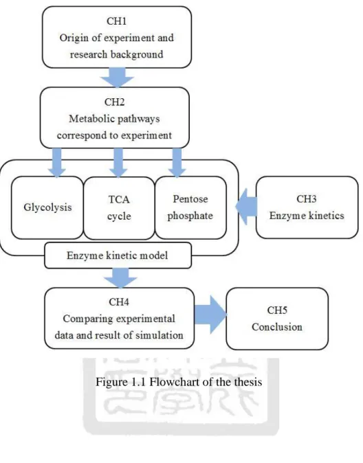
(21) will be covered in this chapter. . Chapter IV derives the equations of different types of enzyme reactions, and solves them numerically to compare with the experimental data.. . Chapter V summaries the findings of the thesis and suggests future works. The following is the flowchart of this thesis. The metabolic pathways we need in the. simulation come from the comparison between experimental observation and literature, and then models for metabolic pathways are built with enzyme kinetics. Simulation of the integrated model is performed to fit the experimental data and finally, the fitting errors are fed back to modify parameters in the model.. 6.

(22) Figure 1.1 Flowchart of the thesis. 7.

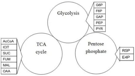
(23) CHAPTER II BASIC CONCEPTS OF CELLULAR METABOLIC PATHWAY. According to the purpose of the experiment to be compared and the underlying principles of the experiment [16], we decide to combine glycolysis, TCA cycle and pentose phosphate pathway in our model. There are two connections between them. The first connection is the conversion of glucose (GLC) into glucose-6-phosphate (G6P), and the production of ribose-5-phosphate (R5P) by reacting G6P with sequent chemical actions. On the other hand, the conversion of pyruvate (PYR) into acetyl CoA (AcCoA) connects glycolysis with TCA cycle. The three metabolic pathways will be discussed respectively and then combined together to describe the change of metabolites of E. coli. Figure 2.1 lists the distribution of metabolites, which appear in this thesis.. Figure 2.1 The distribution of metabolites in each pathway.. 8.

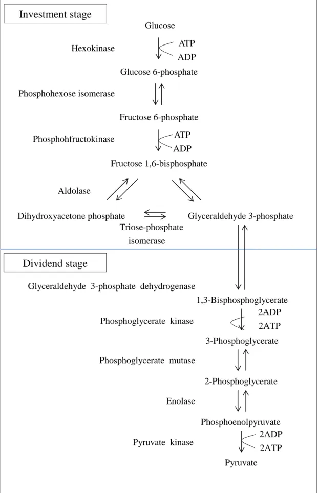
(24) 2.1 Glycolysis The glycolytic pathway (see Figure 2.1) consists of ten enzyme-catalyzed reactions, which use glucose (GLC) as the initial substrate, and split it into two molecules of pyruvate (PYR). We can define two stages of glycolysis from an energy standpoint, the first five of which constitute an “investment stage.” In this stage, glucose is first phosphorylated by ATP to form glucose 6-phosphate (G6P), and then converts into its isomer, fructose 6-phosphate (F6P), which is again phosphorylated to yield fructose 1,6-bisphosphate (FDP) by ATP. Energy in the form of the above two ATPs must be invested to initiate the first stage. In the next step, FDP is split to yield two molecules, glyceraldehyde 3-phosphate (GAP) and dihydroxyacetone phosphate (DHAP). The second stage of glycolysis begins with the molecule of GAP. The second stage, known as the “dividend stage”, is initiated by the conversion of GAP into 1,3-bisphosphoglycerate (PGP) in this sequent reaction. PGP has greater phosphoryl-transfer potential than ATP so that it catalyzes the transfer of the phosphoryl group to ADP. PGP converts to 3-phosphoglycerate (3PG) and governs the synthesis of ATP. A mutase is an enzyme that catalyzes the shift of position of phosphoryl group in the conversion of 3PG into 2-phosphoglycerate (2PG).. 9.

(25) Investment stage Glucose ATP ADP. Hexokinase. Glucose 6-phosphate Phosphohexose isomerase Fructose 6-phosphate ATP ADP. Phosphohfructokinase. Fructose 1,6-bisphosphate Aldolase Dihydroxyacetone phosphate Glyceraldehyde 3-phosphate Triose-phosphate isomerase. Dividend stage Glyceraldehyde 3-phosphate dehydrogenase 1,3-Bisphosphoglycerate 2ADP Phosphoglycerate kinase 2ATP 3-Phosphoglycerate Phosphoglycerate mutase 2-Phosphoglycerate Enolase Phosphoenolpyruvate 2ADP Pyruvate kinase 2ATP Pyruvate. Figure 2.2 The schematic of reactions and the two phases of glycolysis.. 10.

(26) The dehydration of 2PG obviously elevates the transfer potential of phosphoryl group that catalyzes the formation of phosphoenolpyruvate (PEP). PYR is formed and ATP is generated with the help of the high phosphoryl-transfer potential of PEP, which increases the converting force. The reactions of glycolysis introduced above are summarized in Table 2.1, and the net equation for the first five steps is derived as follows: GLC + 2ATP  2GAP + 2ADP.. (2.1.1). The reaction shows that two ATP molecules are consumed for activation processes for each GLC entering the glycolysis. In addition, the net reaction for the second half is:. 2GAP + 2Pi + 4ADP + 2NAD+  2PYR + 4ATP + 2NADH + 2H + + 2H 2O.. (2.1.2). Here two more ATPs and two NADH are generated. The overall net reaction for the ten steps of glycolysis becomes:. GLC + 2Pi + 4ADP + 2NAD+  2PYR + 2ATP + 2NADH + 2H + + 2H 2O.. (2.1.3). In summary, two molecules of ATP and NADH are generated for each GLC, which is split into two molecules of PYR in the process of glycolysis.. 11.

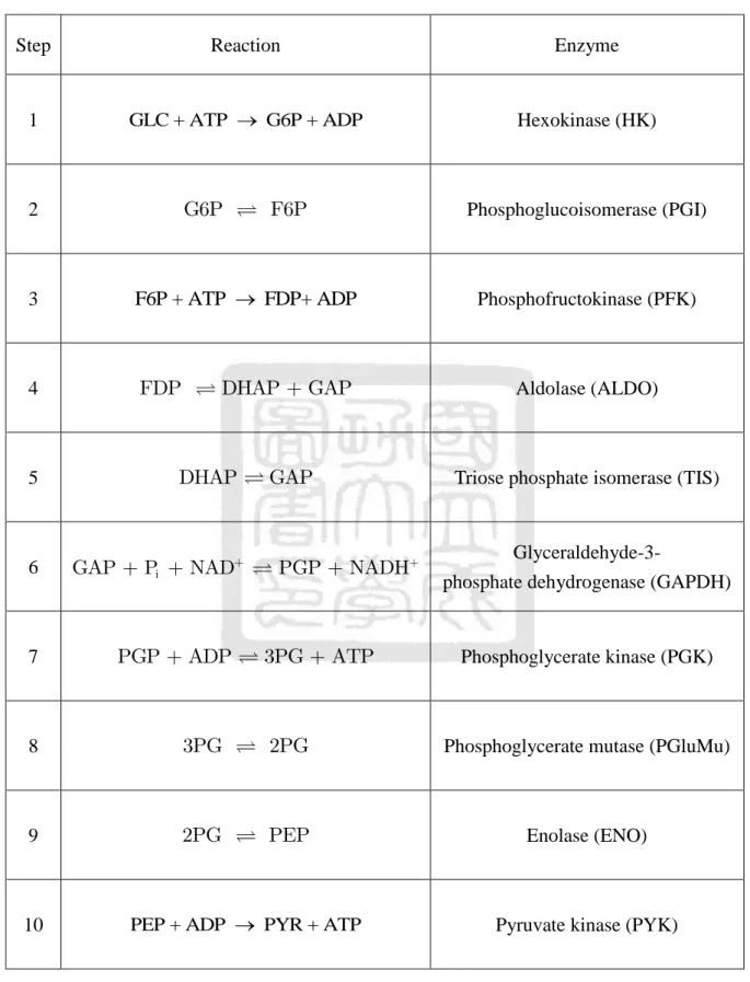
(27) Table 2.1 The reactions of glycolysis with enzymes. Step. Reaction. Enzyme. 1. GLC + ATP  G6P + ADP. Hexokinase (HK). G6P. 2. F6P. 3. F6P + ATP  FDP+ ADP. 4. FDP. 5. 6. 7. Phosphoglucoisomerase (PGI). Phosphofructokinase (PFK). DHAP + GAP. DHAP. GAP + Pi + NAD+. PGP + ADP. Aldolase (ALDO). GAP. Triose phosphate isomerase (TIS). PGP + NADH+. 3PG + ATP. Glyceraldehyde-3phosphate dehydrogenase (GAPDH). Phosphoglycerate kinase (PGK). 8. 3PG. 2PG. Phosphoglycerate mutase (PGluMu). 9. 2PG. PEP. Enolase (ENO). 10. PEP + ADP  PYR + ATP. Pyruvate kinase (PYK). 12.

(28) 2.2 TCA cycle In this section, we will introduce the TCA cycle and the glyoxylate (GOX) cycle.. 2.2.1 TCA cycle In 1937, German biochemist Hans Krebs postulated that a cycle consisting of eight reactions (see Figure 2.3) constitutes the central pathway of aerobic metabolism [16]. The sequence of reactions was proposed by Krebs after a joint research on PYR metabolism with Albert Szent-Györgi and Franz Knoop. The conversion of PYR into acetyl-CoA (AcCoA) is the link between glycolysis and TCA cycle, while AcCoA activates the TCA cycle.. Figure 2.3 The steps of the TCA cycle.. 13.

(29) The reactions of the TCA cycle are illustrated in the following eight steps: Step 1 The cycle begins with the combination of AcCoA with OAA to form citryl CoA, which is a transient intermediate in the form of an energy-rich molecule with thioester bond. The citryl CoA undergoes hydrolysis to produce citrate (CIT) and CoA, rapidly. The reaction is catalyzed by citrate synthase (CS). Step 2 The isomerization of CIT is accomplished by a dehydration to form a double bond intermediate, cis-aconitate (cis-ACO), followed by a hydration to yield isocitrate (ICIT). The enzyme ACO can promote the reversible addition of H2O to cis-ACO such as to produce CIT or ICIT. Step 3 In this reaction, the enzyme ICDH catalyzes the oxidation of hydroxyl group of ICIT results in an unstable intermediate that further decarboxylates to the α-ketoglutarate (α KG). The enzyme ICDH functions with NAD+ as an electron accepter. NAD+ and NADH are the most often cofactors for the transfer of hydroxyl and keto groups. Step 4 More complicated than the previous step, it is another oxidative decarboxylation which requires five chemical steps involving three enzymes and their cofactors. αKG is. 14.

(30) converted to form thioester bond of succinyl-CoA (SCoA) and CO2 by the action of theα KGDH. Step 5 SCoA is an energy-rich thioester compound. In this step, the energy is transformed from a thioester bond to ATP or GTP. There are two forms of succinyl-CoA synthetase (SCS) in higher animals; one prefers ADP as a phosphoryl-group accepter and the other prefers GDP as the accepter. By contrast, only ADP can be treated as the accepter in plants and microorganism. It appears that ATP or GTP is generated by substrate-level phosphorylation. The enzyme that catalyzes this reaction converts SCoA to succinate (SUC) and CoA. Step 6 The succinate formed from SCoA is oxidized to fumarate (FUM) in a reaction catalyzed by succinate dehydrogenase (SDH), which like aconitase (ACOS) is an iron-sulfur protein. The enzyme with an FAD prosthetic group serves as the electron accepter in oxidations that remove two hydrogen atoms from a substrate. Step 7 The hydration of FUM to L-malate (MAL) is a reversible reaction. The enzyme, fumarase (FUMe), catalyzes a stereospecific trans-addition of H+ and OH-. The OH- group joins to only one side of the double bond of FUM such that only the L stereoisomer of. 15.

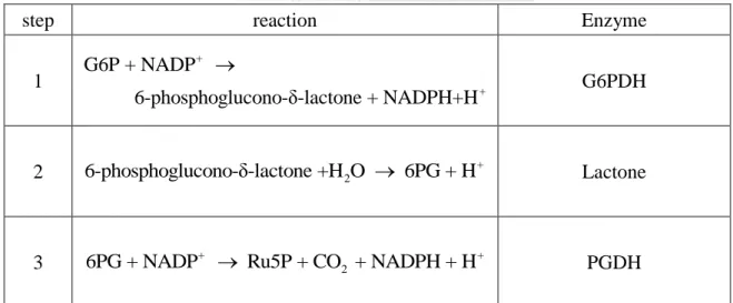
(31) MAL can be formed. Step 8 In the last reaction of TCA cycle, L-MAL is oxidized to form OAA. It is catalyzed by malate dehydrogenase (MDH), and is linked to the coenzyme NAD+. Adding the eight steps above, the net reaction for the TCA cycle appears as. AcCoA + 3NAD+ + FAD + ADP(GDP) + Pi + 2H 2O  2CO 2 + 3NADH + 3H + + FADH 2 + ATP(GTP) + CoA. The function of the overall TCA cycle can be summarized as following and the individual reactions in the cycle are listed sequentially in Table 2.2. 1. AcCoA enters and two carbons leave the cycle as CO2 in different steps. 2. Three molecules of NAD+ are reduced to NADH by dehydrogenase-catalyzed reactions. 3. One molecule of FAD is reduced to FADH2. 4. The energy stored in a CoA thioester is transferred to the phosphoanhydride bond in ATP or GTP. Table 2.2 The reactions and their related enzymes in the TCA cycle. Step 1. Reaction. AcCoA + OAA + H2O. Enzyme. CIT + CoA. 16. CS.

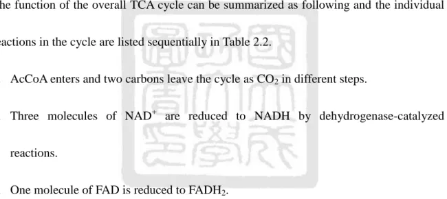
(32) 2. CIT. 3. ICIT + NAD+. 4. 5. 6. ICIT. αKG + CO2 + NADH + H+. αKG + NAD+ +CoA SCoA + CO2 + NADH + H+. SCoA + Pi + ADP(GDP) SUC + ATP(GTP) + CoA. SUC + FAD. FUM + H2O. 7. 8. cis-ACO. L-MAL. + NAD+. ACOS. ICDH. αKGDH. SCS. FUM + FADH2. SDH. L-MAL. FUMe. OAA + NADH + H+. MDH. 2.2.2 Glyoxylate cycle Plants and some microorganisms, such as E. coli and Pseudomonas, can utilize the compound acetate as an energy-rich fuel and as a source of phosphoenolpyruvate for carbohydrate synthesis. This process is called Glyoxylate (GOX) cycle as shown in Figure 2.4. However, GOX cycle is not present in higher animals. The GOX cycle is based on a TCA cycle modified by a reaction that forms SUC from two molecules of AcCoA.. 17.

(33) Figure 2.4 Glyoxylate cycle. The GOX cycle begins with the condensation of AcCoA and OAA to form CIT, which is isomerized by dehydration and hydration to yield ICIT. In the next step, a branch to the GOX cycle begins. Instead of breakdown of the ICIT by ICDH, ICIT now undergoes the cleavage by isocitrate lyase (ICL) and is split into SUC and GOX. SUC is expelled from the cycle and used by the plant or microorganism for other purpose. GOX then condenses with AcCoA to produce MAL catalyzed by malate synthase (MS) and CoA. Finally, the MAL is subsequently oxidized to OAA to start another turn of the cycle. As a summary of the GOX cycle, we arrange the reactions in Table 2.3 and express the net reaction as. 18.

(34) 2AcCoA + NAD+ + 2H2O  SUC + 2CoA + NADH + H + . Comparing with TCA cycle, we find that two AcCoAs are converted into one SUC in the glyoxylate cycle. Later, we will combine the TCA cycle with the glyoxylate cycle as a part of the metabolic sequences (see Figure 2.5) [8]. Table 2.3 The reactions of glyoxylate cycle. Step 1 2 3. Reaction. AcCoA + OAA + H2O. CIT ICIT. Enzyme. CIT + CoA. ICIT SUC+GOX. 4. GOX + AcCoA + H2O. 5. MAL + NAD+. MAL + CoA. OAA + NADH + H+. CS ACOS ICL MS MDH. Figure 2.5 TCA cycle is combined with glyoxylate bypass.. 19.

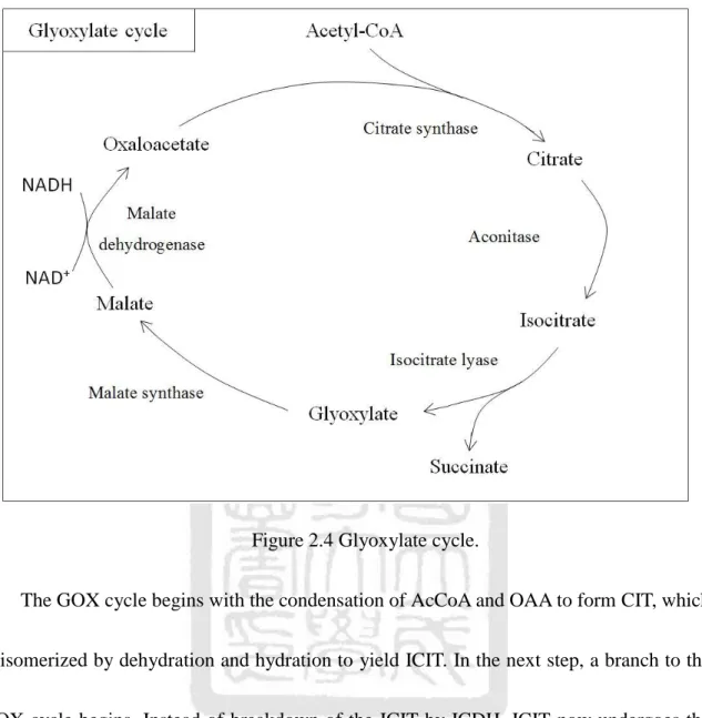
(35) 2.3 Pentose Phosphate Pathway In most animals, the major function of glycolysis is to oxidize GLC to PYR, which then participates the following metabolism via continued oxidation in TCA cycle and cellular respiration. GLC has a secondary pathway, which leads to specialized production needed by some animal and plant cells. The pentose phosphate (PP) pathway (see Figure 2.6 and 2.7) produces the ribose-5-phosphate (R5P) and reduces energy in the form of NADPH by oxidizing GLC. This pathway consists of two phases: (1) the oxidative generation of NADPH and (2) the non-oxidative inter-conversion of sugars.. Figure 2.6 Oxidative phase of pentose phosphate pathway. In the oxidative phase, the GLC is transferred to R5P by a five-reaction oxidative. 20.

(36) process. The first reaction is the phosphorylation of glucose by ATP to form G6P, which in turn is dehydrogenated by glucose 6-phosphate-dehydrogenase (G6PDH) to form 6-phosphoglucono-δ-lactone. The lactone is hydrolyzed by a specific lactonase to the free acid 6-phosphogluconate, which then undergoes dehydrogenation and decarboxylation by 6-phosphogluconate dehydrogenase (PGDH) to form the D-ribulose-5-phosphate (D-Ru5P). Finally, ribulose-5-phosphate isomerase (RPI) converts D-Ru5P to its aldose isomer, ribose-5-phosphate (R5P). The overall equation of the oxidative phase of the PP pathway is:. G6P + 2NADP+ + H2O  R5P + CO2 + 2NADPH + 2H + .. (2.3.1). The net result of the oxidization of each molecule of G6P is to produce two molecules of NADPH and one molecule of R5P. The overall reaction is listed in Table 2.4. Table 2.4 The reaction of oxidative phase of pentose phosphate pathway. step 1. reaction. Enzyme. G6P + NADP+  6-phosphoglucono-δ-lactone + NADPH+H +. G6PDH. 2. 6-phosphoglucono-δ-lactone +H 2O  6PG + H +. Lactone. 3. 6PG + NADP+  Ru5P + CO2 + NADPH + H +. PGDH. 21.

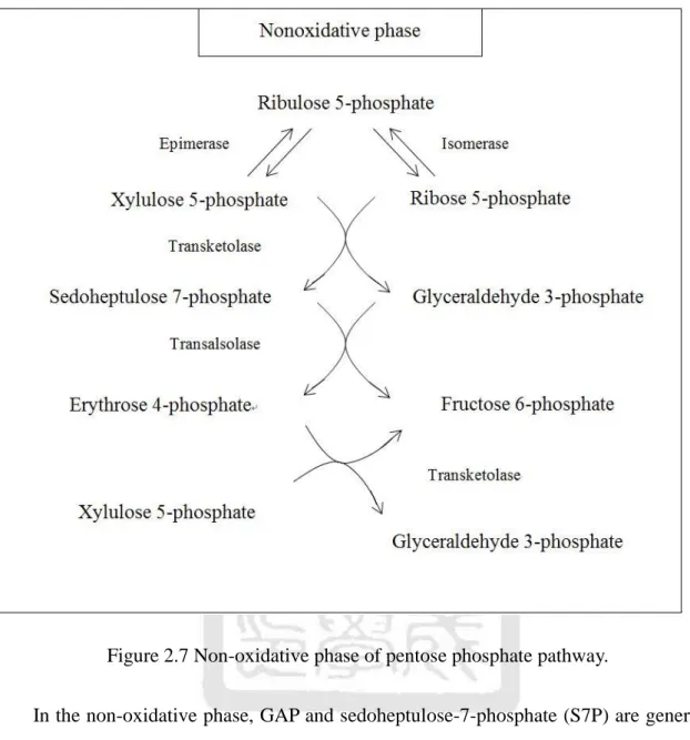
(37) Figure 2.7 Non-oxidative phase of pentose phosphate pathway. In the non-oxidative phase, GAP and sedoheptulose-7-phosphate (S7P) are generated by the transketolase (TKTA), which catalyzes the transfer of two carbons in xylulose-5-phosphate (X5P) to R5P. Transaldolase (TAL) then catalyzes a reaction that a three-carbon fragment is removed from S7P, which is then condensed with GAP to form F6P and erythrose-4-phosphate (E4P). Finally, TKTB acts again to transfer E4P and X5P into F6P and GAP. All the reactions of the non-oxidative part are readily reversible, as listed in Table 2.5. The net equation describing the non-oxidative phase is:. 22.

(38) 3R5P. 2F6P + GAP.. (2.3.2). Thus, excessive R5P formed by the PP pathway can be completely converted into glycolytic intermediates. Table 2.5 The reactions of the non-oxidative phase of pentose phosphate pathway. step. reaction. Enzyme. 1. Ru5P. R5P. RPI. 2. Ru5P. X5P. Phosphopentose epimerase (RPE). 3. 4. 5. X5P + R5P. S7P + GAP. X5P + E4P. S7P + GAP. TKTA. F6P + E4P. Transaldolase. F6P + GAP. TKTB. The three metabolic pathways we discuss above are the main pathways occurring in biochemistry. By combining the three metabolic pathways, we wish to construct a model to describe the dynamic behavior of the metabolites of E. coli in the knockout experiment [4]. In the next chapter, we will illustrate the basic theories of enzyme kinetics, categorize the corresponding reactions, and use them to build the mathematical model. We will combine the three metabolic processes in Figure 3.5 and list their related differential equations in the end of chapter 3. 23.

(39) CHAPTER III ENZYME KINETICS. In this chapter, we will study the rate equations for the change in metabolic concentrations. When initial rates are used, the influential factors, such as substrate concentration, catalytic concentration and inhibitor effect, must be considered. We will introduce Michaelis-Menten equation and examine the effect of inhibitors in sequence, and then combine both of them to construct a mathematical model, which will be used in the next chapter to simulate the change of metabolites by comparing with the result of experiment.. 3.1 Michaelis-Menten Equation Generally, enzymes catalyze the reaction that helps to convert other molecules called substrates into product, but they themselves are not changed by the reaction. Enzyme reactions do not follow the law of mass action directly. At relatively low concentrations of substrate, the initial reaction rate increases with increasing substrate concentration as expected. At higher concentrations of substrate, the rate increases only to a certain extent, reaching a maximal reaction velocity. In 1913, Leonor Michaelis and Maud Menten [1] explained the catalytic behavior, including enzymes, which can be described by a substrate saturation effect. They proposed a general theory for enzyme action and derived a. 24.

(40) mathematical equation to express the experimental data and to calculate rate constants. Michaelis and Menten proposed that enzyme molecules, E, and substrate molecules, S, combine in a fast and reversible step to form an ES complex, as shown in Figure 3.1:. Figure 3.1 The mechanism of Michaelis-Menten equation. The reaction scheme can be written by E. S. k1 k-1. k2. ES. E. P.. (3.1.1). The terms 𝑘1 , 𝑘−1 , and 𝑘2 are, respectively, the constants for binding to the enzyme, substrate unbinding, and conversion to product. According to the law of mass action, there is a system of four ordinary differential equations that define the rate of change of reactants with time t: d S   -k1  E  S   k-1  ES  , dt. (3.1.2a). d E  -k1  E  S   k-1  ES   k2  ES  , dt. (3.1.2b). d  ES   k1  E  S  - k-1  ES  - k2  ES  , dt. (3.1.2c). d  P  k2  ES  , dt. (3.1.2d). where [ . ] denotes the concentration of reactants. Michaelis and Menten assumed. 25.

(41) that the substrate S is in instantaneous equilibrium with the complex, i.e.. k1, k-1. k2 .. (3.1.3). And thus. k1  E  S   k-1  ES .. (3.1.4). In this mechanism, the enzyme is a catalyst, which only facilitates the reaction, so that total concentration [𝐸𝑇 ] = [𝐸] + [𝐸𝑆] is a constant. Then [ES] can be solved from Eq.(3.1.4) as k1  ET    ES   S   k-1  ES . .  ES  .  ET  S  . k1 / k1   S . (3.1.5). Substituting Eq.(3.1.5) into Eq.(3.1.2d), we obtain d  P dt. . k2  ET  S . k1 / k1   S . .. Let 𝐾𝑠 be an equilibrium constant for substrate dissociation that equals to. (3.1.6) 𝑘−1 𝑘1. , and. 𝑉𝑚𝑎𝑥 = 𝑘2 [𝐸𝑇 ] be the maximum velocity of the reaction. So we can rewrite the Eq.(3.1.6) v. d  P  Vmax  S   , dt KS   S . (3.1.7). which is generally known as the Michaelis-Menten equation. Based on the same reaction mechanism, an alternative hypothesis was suggested by Briggs and Haldane in 1925: if the concentration of enzyme is much less than substrate, then very shortly after mixing E and S, a steady state will be reached in which the. 26.

(42) concentration of the intermediate is constant, that is d  ES   0. dt. (3.1.8). Then we can rewrite use Eq.(3.1.2c) as. k1  E  S    k-1  k2   ES .. (3.1.9). From which [ES] can be solved with the relation [𝐸] = [𝐸𝑇 ] − [𝐸𝑆] as.  ES  .  ET  S  ,  k-1  k2  / k1   S . (3.1.10). The substitution of Eq.(3.1.10) into Eq.(3.1.2d) yields d  P dt. . k2  ET  S .  k-1  k2  / k1   S . With the introduction of the Michaelis constant 𝐾𝑀 = v. d  P  Vmax  S   . dt KM  S . (3.1.11). .. 𝑘−1 +𝑘2 𝑘1. , Eq.(3.1.11) becomes. (3.1.12). Comparing with Eq.(3.1.7), we see that the rate in Eq. (3.1.12) is similar than the equilibrium hypothesis. When 𝑘1 , 𝑘−1 ≫ 𝑘2 , we have 𝐾𝑀 → 𝐾𝑆 and thus the two rates in Eq. (3.1.7) and (3.1.12) become identical.. 3.2 Enzyme Inhibition According to their extent of interaction with enzymes, two broad classes of inhibitors have been identified, irreversible and reversible. An irreversible inhibitor dissociates very slowly from its target enzyme because it has become tightly bound to the enzyme, either. 27.

(43) covalently or noncovalently. Therefore, the enzyme is rendered permanently inactive. Reversible inhibitors are those that can combine with and dissociate from an enzyme and render the enzyme inactive when bound. Three common types of reversible inhibitors are classified as competitive, uncompetitive, and noncompetitive[17].. 3.2.1 Competitive Inhibitor This type of enzyme inhibition means that either the inhibitor or the substrate can bind the enzyme but not at the same time.. Figure 3.2 The mechanism of competitive inhibitor. As shown in Figure 3.2, the reaction scheme is: E. S. k1 k-1. k2. ES. E. P,. ki   EI . E  I   k i. (3.2.1a) (3.2.1b). We still need four ordinary differential equations to describe the reaction in Eq.(3.2.1) as those listed in Eq.(3.1.2). We define the equilibrium constant. 28.

(44) KI . ki  E  I   , ki  EI . and thus.  EI    E  I  / K I .. (3.2.2). According to the steady-state assumption d  ES  dt. 0,. we have k1  E  S    k1  k2   ES . . E .  k1  k2   ES  . k1  S . (3.2.3). Combining Eq.(3.2.2) and Eq.(3.2.3) to form the total enzyme concentration, we get.  ET    ES    E    EI    ES    E  .  E  I  KI.  I    k1  k2   ES  1   I     ES    E  1     ES     k1  S   KI   KI . (3.2.4).  k  k   I     ES  1  1 2 1   .  k1  S   K I    Finally the rate of production of the product P is d  P dt.  k2  ES  . k2  ET  S  . k1  k2   S   1   I  / K I  k1. With the definitions. Vmax  k2  ET  , K M  Eq.(3.2.5) can be rewritten as. 29. k1  k2 , k1. (3.2.5).

(45) v. d  P dt. . Vm a x S .  S   K M 1   I  / K I . .. (3.2.6). 3.2.2 Uncompetitive Inhibitor An uncompetitive inhibitor binds only the substrate-enzyme complex. The substrate facilitates the binding of the inhibitor to the enzyme. According to figure 3.3, the reactions can be represented by E. S. k1 k-1. k2. ES. E. P,.   ESI . ES  I  ki. k i. (3.2.7a) (3.2.7b). Defining the equilibrium constant KI .  ES  I  .  ESI . (3.2.8). Figure 3.3 The mechanism of uncompetitive inhibitor. Combining Eq.(3.2.3), Eq.(3.2.8) and the constant concentration of enzyme, we obtain. 30.

(46)  ES  .  ET  S  . I    1   S   KM . (3.2.9). KM . The rate of appearance of P depends on the concentration of the inhibitor I in the following:. v. d  P Vmax  S   . dt I    1  K   S   K M M  . (3.2.10). 3.2.3 Noncompetitive inhibitor Noncompetitive inhibition is also called mixing inhibition; the inhibitor can bind either the free enzyme or the enzyme-substrate complex. We must consider three reaction schemes for noncompetitive inhibitor as shown in Figure 3.4.. Figure 3.4 The mechanism of noncompetitive inhibitor. The reactions are described by E. S. k1 k-1. k2. ES. 31. E. P,. (3.2.11a).

(47) ki 1  E  I  EI ,. (3.2.11b). ki 2    ESI . ES  I  . (3.2.11c). k i 1. k i 2. From Eq.(3.2.11b) and Eq.(3.2.11c), we can define KI1 . ki1  E  I   , ki 1  EI . (3.2.12). KI 2 . ki 2  ES  I   . ki 2  ESI . (3.2.13). The total enzyme concentration will be.  ET    E    ES    EI    ESI  ,. (3.2.14). Substituting Eq.(3.2.3), Eq.(3.2.12) and (3.2.13) into Eq.(3.2.14), we obtain.  ES  .  ET  S .  I   k  k  I    S  1    1 2 1   k1  K I 1   KI 2 . .. (3.2.15). Depending on the concentration of the inhibitor I, the rate of the reaction can be expressed as the following form:. v. Vmax  S  . I  I       S  1    K M 1    KI 2   KI1 . (3.2.16). 3.3 Kinetics Model in Metabolic Pathway Based on the theories proposed in the above two sections, we can build up the mathematical model for some reaction. But it is not applicable to all biochemical reactions. Owing to the order of addition of reactants to and release of products from the enzyme. 32.

(48) active site, kinetics mechanisms fall into two broad categories [17]. . Sequential mechanisms are characterized by the fact that all reactants must be bound to an enzyme before any reaction occurs.. . Ping-Pong mechanics denotes the situation that a product is released between the consecutive additions of the two substrates with the enzyme.. Sequential mechanisms can be termed either order, when there is a compulsory order of substrate addition and product released, or random, when there is not. The rapid equilibrium indicates a special case in which the equilibrium between an enzyme-reactant and a free-reactant is established. In ping pong mechanisms, the reaction order for a given enzyme is obtained from the number of reactants in the both reaction directions. The terms Uni, Bi, Ter, and Quad are used for the enzyme-catalyzed reactions with one, two, three, and four reactants in a given reaction direction. For example, a reaction having a reactant A and two products P and Q, are thus called Uni-Bi reaction. We list the classification of reactions in Table 3.1 to help for determining the characteristic of reaction and for choosing a proper model for it. Table 3.1 Classification of the kinetic mechanism. Mechanism Sequential. Type. Property. order. Obligatory order. 33.

(49) Random. Distinct binding. Rapid equilibrium. Special case in equilibrium. Uni. One reactant in a direction. Bi. Two reactants in a direction. Ter. Three reactants in a direction. Quad. Four reactants in a direction. Ping pong. Besides the categories of reaction, Chassagnole et al. [11] and Kadir et al. [12] built the model to describe E. coli. According to these methods and theories, we modify the equations by combining Michaelis-Menten equations and enzyme inhibition, and consider an example for irreversible Bi-Uni (two substrates and one product) system to derive the equations. Figure 3.5 demonstrates a reaction with competitive inhibition. Figure 3.5 The reaction for a Bi-Uni system with competitive inhibition. The reaction can be written as. 34.

(50) E. A. E. B. k1 k. 1. k2 k. 2. k2. EA. B. EB. A. E. k. I. 2. k1 k. 1. kI 1 k. I1. EAB. k3. EQ. P,. (3.3.1a). EAB. k3. EQ. P,. (3.3.1b). EI ,. (3.3.1c). where α is the proportional constant of combining the same substrates. Owing to the principle of mass action, we obtain the equations d  A  k1  E  A  k1  EA   k1  EB  A   k1  EAB  , dt d  B dt.  k2  E  B   k2  EB    k2  EA B    k2  EAB  .. (3.3.2a) (3.3.2b). We consider the steady-state condition,.  EA . k1  E  A , k1. (3.3.3a).  EB . k2  E  B  , k2. (3.3.3b).  E  I   k I 1 .  EI  k I 1. (3.3.3c). KI . and introduce the definitions. Ka . k1 k , Kb  2 . k1 k2. Substituting (3.3.3) into the relation of total enzyme concentration, we obtain.  ET    E   Ka  E  A  Kb  E  B    EAB  .  E  I  KI.   I    EAB   E   1  K a  A  K b  B      KI     1  I    1 ,   EAB    1  K a  A  K b  B     KI    K a Kb  A B  . 35.

(51) from which [𝐸. ] can be solved as.  EAB .  ET  A B .  1  I    A B  1  K a  A  Kb  B         K I   K a Kb  . .. Finally, substituting it into the product equation yields. d  P Vmax  A B   . dt  1   I    1  K a  A  Kb  B   K    A B   I   Ka Kb  . (3.3.4). Next, we proceed to consider the reaction of a Bi-Uni system with an uncompetitive inhibitor as shown in Figure 3.6.. Figure 3.6 The reaction for a Bi-Uni system with uncompetitive inhibition. Unlike the case of a competitive inhibitor, there are three more inhibition equations EA. I. EB. I. kI 1 k. I1. kI 2 k. I2. 36. EAI ,. (3.3.5a). EBI ,. (3.3.5b).

(52) EAB. kI 3. I. k. I3. EABI .. (3.3.5c). Similarly, we define the equilibrium constants. KI1 . k I 1 k k , KI 2   I 2 , KI 3   I 3 . kI1 kI 2 kI 3. and substitute (3.3.3) into the equation of total concentration to obtain.  ET    E   Ka  E  A  Kb  E  B    EAB  .  EA I    EB  I    EAB  I  KI1. KI 2. KI 3.    I    K B 1   I     EAB 1   I   ,   E   1  K a  A  1       b   K K I 1 I 2      KI 3    From which [𝐸. ] can be solved as.  EAB .  ET  A B  . I  I  I        1  K a  A  1     Kb  B   1     A B   1  . KI1 . . KI 2 . . KI 3 . Under the assumption. KI . k I 1 k I 2 k I 3   , kI 1 kI 2 kI 3. we can get.  EAB  .  ET  A B .  I   1   K a  A  Kb  B    A B   1  K I  . .. So the rate equation of product becomes. d  P  dt. Vmax  A B .  I   1   K a  A  Kb  B    A B   1    KI . .. (3.3.6). The third type of reactions to be considered is the noncompetitive inhibition, which is. 37.

(53) a combination of competitive and uncompetitive inhibitors, as shown in Figure 3.7.. Figure 3.7 The reaction for a Bi-Uni system with a noncompetitive inhibition. The corresponding inhibition equations are described by E EB. kI 1. I I. k kI 3 k. I3. I1. EI , EBI ,. EA. kI 2. I. EAB. k. I. EAI ,. I2. kI 4 k. I4. (3.3.7a). EABI .. (3.3.7b). In terms of the equilibrium constants. KI1 . k I 1 k k k , KI 2   I 2 , KI 3   I 3 , KI 4   I 4 , kI 1 kI 2 kI 3 kI 4. the total enzyme concentration can be expressed by.  ET    E   K a  E  A  Kb  E  B    EAB  .  E  I    EA I    EB  I    EAB  I  KI1. KI 2. KI 3. KI 4.  I     I    K B 1   I     EAB 1   I     E   1   K a  A  1         b    K K K I 1 I 2 I 3        KI 4    .  EAB   1   I    K A 1   I    K B 1   I     1   I   ,        a   b   K a K b  A B    K I 1   KI 2   KI 3    KI 4 . From which [𝐸. ] can be solved to be. 38.

(54)  EAB  .  ET  A B  .  I  I  I   I          1      A B   1    K a  A  1    Kb  B   1  . 1 K a Kb  . KI1 . . KI 2 . . KI 3  . . KI 4 . With a further approximation that all the equilibrium constants are equal. KI . k I 1 k I 2 k I 3 k I 4    , kI 1 kI 2 kI 3 kI 4. we obtain the product equation as. d  P Vmax  A B   . dt  1  I   1  Ka  A  Kb  B    A B   1  K   I   K a Kb . (3.3.8). We have shown above how to build the rate equations by the kinetics model that obeys the law of conservation of mass for metabolites. Following the same procedures, we will introduce the rate equation of each reaction after deriving the ordinary differential equations of metabolites in E. coli. A mathematical model will be proposed to describe the three main metabolic pathways as shown in Figure 3.8 under the following assumptions: 1. TIS is well in equilibrium state so that GAP and DHAP are lumped together. 2. A sequence of enzymatic reactions is in the order of PGK, PGluMu and ENO, which are considered to be in equilibrium so that there is only one reaction from GAP to PEP.. 39.

(55) Figure 3.8 The three metabolic pathways considered in the model of E. coli.. 40.

(56) The general dynamic equation can be described by the mass balance as: d. i. dt. vij rj j. i. ,. where [ ] is the concentration of the ith metabolite, μ is the rate of cell growth, the stoichiometry, and. is. is the rate of the jth reaction. According to Figure 3.8, we can. obtain the ordinary differential equations as follows: d X   X  dt. (3.3.9a). d GLCex   vPTS  X  dt. (3.3.9b). d G 6 P   vPTS  vPGI  vG 6 PDH   G P  dt. (3.3.9c). d  F 6P   vPGI  vPFK  vTKTB  vTAL    F  P  dt. (3.3.9d). d  FDP   vPFK  v ALDO    FDP  dt. (3.3.9e). d GAP   2v ALDO  vGAPDH  vTKTA  vTKTB  vTAL   GAP  dt. (3.3.9f). d  PEP   vGAPDH  vPCK  vPTS  vPYK  vPPC    PEP  dt. (3.3.9g). d  PYR   vPYK  vPTS  vMEZ  vPDH    PYR  dt. (3.3.9h). d  AcCoA  vPDH  v ACS  vCS  vPTA    AcCoA dt. (3.3.9i). d  ICIT   vCS  vICDH  vICL    ICIT  dt. (3.3.9j). d  KG   vICDH  v KGDH    KG  dt. (3.3.9k). d  SUC   v KGDH  vICL  vSDH    SUC  dt. (3.3.9l). d  FUM   vSDH  vFUM    FUM  dt. (3.3.9m). 41.

(57) d  MAL  vFUM  vMS  vMDH  vMEZ    MAL dt. (3.3.9n). d OAA  vMDH  vPPC  vCS  vPCK   OAA dt. (3.3.9o). d GOX   vICL  vMS   GOX  dt. (3.3.9p). d  ACP   vPTA  v ACK    ACP  dt. (3.3.9q). d  ACEex    v ACK  v ACS   X  dt. (3.3.9r). d 6PG   vG 6 PDH  vPGDH   6PG  dt. (3.3.9s). d  Ru5P   vPGDH  vRPE  vRPI    Ru5P  dt. (3.3.9t). d  R 5P   vRPI  vTKTA    R5P  dt. (3.3.9u). d  X 5P   vRPE  vTKTA  vTKTB    X 5P  dt. (3.3.9v). d  S 7P  vTKTA  vTAL    S 7 P  dt. (3.3.9w). d  E 4P  vTAL  vTKTB    E 4 P  dt. (3.3.9x). There are twenty-four equations included in the whole reaction. We will apply the Michaelis-Menten equations combined with the three types of enzyme inhibition to the metabolic pathways considered in Figure 3.8. Each rate in Eq. (3.3.9) will be derived according to the number of reactant, inhibition category, reversibility and cooperation, and the detailed derivations are listed in appendix A. In the following, we take the rate equation of enzyme PTS as an example to illustrate the underlying procedures. The reaction to be considered is 𝑃𝑇𝑆. 𝑃𝐸𝑃 + 𝐺𝐿𝐶 → 𝑃𝑌𝑅 + 𝐺6𝑃, 42.

(58) and the detailed reaction can be described by.    EA   B      EAB  ,  E    A   k k. (3.3.10a).   EB   A     EAB  ,  E    B   k k. (3.3.10b).  k2. k1. 1. 2.  k1. k2. 2. 1. where A, B, E denote PEP, GLC, PTS, respectively. According to the types of inhibition, we can list the inhibition equations as: E. Q. EA. Q. EB. Q. EAB. Q. kI 1 k. I1. kI 2 k. I2. kI 3 k. I3. kI 4 k. I4. EQ ,. (3.3.11a). EAQ ,. (3.3.11b). EBQ ,. (3.3.11c). EABQ ,. (3.3.11d). where Q denotes the product and also acts as an inhibitor in this reaction. Meanwhile, on the basis of the conservation of the total enzyme concentration, we can get.  ET    E    EQ   EA   EB   EAQ   EBQ   EABQ.. (3.3.12). Substituting eq. (3.3.11) and (3.3.12) into the noncompetitive inhibition equation, we obtain.  EAB . where 𝐾𝑎1 =. 1.  ET . Q    Ka1  Ka 2  A  Ka 3  B    A B  1  K   G6P   , 𝐾𝑎2 =. 1. , 𝐾𝑎 =. 1. cooperation, the rate equation has to be modified as. 43. ,. (3.3.13). . Because G6P has a n-type of.

(59) v. where we define. k3  ET  A B . n  Q    Ka1  Ka 2  A  Ka 3  B   A B  1  K  G6P  . 𝑚𝑎𝑥. ,. (3.3.14). = 𝑘 [𝐸𝑇 ].. After the rate equations derived from Appendix A are all substituted into Eq. (3.3.9), we get the complete differential equations that describe the three metabolic pathways in Figure 3.8. These equations will be implemented in the numerical environment of Matlab. All the constants involved in the equations have to be evaluated numerically, before we can solve the set of differential equations. The numerical values of the constants used in the simulation are listed in Table 4.2, which are quoted from Chassagnole [11] and Kadir [12]. In the next chapter, we will report the simulation results and compare them with the experimental data to verify the proposed model.. 44.

(60) CHAPTER IV EXPERIMENTAL DATA AND SIMULATION VERIFICATION. After having discussed the main metabolic pathways and the related mathematical model, we will solve the differential equations in this chapter to obtain the changes of metabolites in E. coli O157:H7 and to compare them with the experimental results. Firstly, we introduce the experimental data and find the matching error with the numerical predictions. The matching error is then fed back to a least-square algorithm to adjust the parameters in the model so that the matching error is decreasing as the iteration process goes on.. 4.1 Experimental Procedure and Measurement The experiment was performed by Professor C. S. Chen at Department of Biochemistry and Molecular Biology of National Cheng Kung University. EDL933 is the original culture of E. coli O157:H7, while SDHA is the mutative culture by replacing the enzyme SDH with the antibiotic resistance gene. The difference in the concentration of metabolites between the two cultures is then recorded. The experimental procedures are outlined below. 1. The EDL933 culture is made from the clinical isolations of the E. coli O157:H7 at the. 45.

(61) Bioresource Collection and Research Center. 2. The lambda Red recombination system provides a simple and versatile method for replacing enzyme SDH by the antibiotic resistance gene, Kanamycin. 3. The EDL933 and SDHA mutant are growing in the Luria-Bertani(LB) broth at 37°C and shaking at 220 rpm overnight without adding further antibiotics to the LB broth. 4. Rotate the two cultures in a centrifuge at 8000 rpm for 15min at 4°C. 5. 40ml of bacteria culture broth are collected. Remove the broth and suspend the cell pellet in 5ml deionized water on ice. 6. The pellet is re-suspended in 0.5ml deionized water, and then stored at -80°C to get bacteria powder by freeze drying. After the above preparation procedures for the two samples, the samples are then analyzed through the following measurement steps. 1. Each sample (powder) is added with 600 μl of 100% MeOH as a ratio of 1 to 3, and metabolites are extracted by vortex for 5 min. 2. After 10 min centrifugation at 14,000 rpm, 200 μl of supernatant is taken for vacuum dry at room temperature. 3. The dry sample is reconstituted in 100 μl of 80% MeOH and then centrifuged at 14,000 rpm for 10 min. 4. The supernatant is collected as a sample and subjected to LC-ESI-MS analysis. The. 46.

(62) acquired data are processed by TargetAnalysis and DataAnalysis software and summarized in an integrated area of signals. Found compounds are selected with the tolerance of LC peaks within 0.3 min and area higher than 1000 counts from established compound identities. After deleting those measurements with large deviation from the mean value, the remaining measurements are averaged, respectively,. for the data of E. coli O157:H7. EDL933 and SDHA. The relative changes of the metabolites in SDHA with respect to those in EDL933 are listed in Table 4.1. Table 4.1 The relative changes of metabolites between EDL933 and SDHA. Metabolite. EDL933. SDHA. Percent increase. G6P. 6217.088. 5668.813. -8.82%. F6P. 6217.088. 5668.813. -8.82%. GAP. 4698.46. 3981.97. -15.25%. PEP. 51912. 50077. -3.54%. PYR. 18415.79. 13060.11. -29.08%. AcCoA. 2570.83. 1052.50. -59.06%. ICIT. 37661. 24729. -34.34%. SUC. 37177.27. 79873.87. 118.96%. FUM. 108541.9. 32453.8. -70.10%. MAL. 1895.3. 2500.1. 31.91%. OAA. 2969. 2733. -7.94%. R5P. 1719. 1555. -9.54%. E4P. 1182.9. 1063.6. -10.08%. The relative changes of metabolites between EDL933 and SDHA will be set as the target values, while we adjust the simulation model. In the next section, the model is. 47.

(63) initially simulated with parameters given by [11] and [12]. We then employ the leastsquare algorithm in Section 4.3 to adjust the parameters so that the simulation results approach the target values given by the measurements in Table 4.1. Finally, in Section 4.4 we will used the modified model to predict the new effects caused by other mutants.. 4.2. Initial Simulation Based on Parameters from Literature The 24 differential equations as expressed by Eq. (3.3.9) involve many free. parameters, whose numerical values have to be assigned in advance before we can solve the model for simulation. The initiate our simulation, the parameters given by Chassagnole [11] and Kadir [12], as listed in Table 4.2, will be regarded as the first guess of the correct parameters in order to best fit the measurement data in Table 4.1. With the parameters given by Table 4.2, the set of differential equations (3.3.9) are solved simultaneously to give the time responses of the various metabolites, such as G6P, F6P, GAP, PEP, PYR, AcCoA, ICIT, SUC, FUM, MAL, OAA, R5P and E4P. The results are shown in Figure 4.1 for the metabolites in EDL933 and in Figure 4.2 for the metabolites in SDHA.. 48.

(64) Figure 4.1 Initial simulations of metabolites in E. coli EDL933.. 49.

(65) Figure 4.2 Initial simulations of metabolites in E. coli SDHA.. 50.

(66) Table 4.2 Kinetic parameters[11][12]. Enzyme. Parameters. PTS. vmax Ka1 Ka2. 469786.8 mM/min 3082.3 mM 0.01 mM. Ka3 nG6P KG6P. 245.3 mM 3.66 2.15 mM. PGI. vmax KG6Pm. 39059.27 mM/min 2.9 mM. Keq KG6P,6PGinh. 0.1725 0.2 mM. KF6Pm. 0.266 mM. KF6P,6PGinh. 0.2 mM. PFK. vmax KATP,ADP Ka,ADP,AMP Kb,ADP,AMP. 110435.08 mM/min 4.27 mM 1.0546 mM 1.4514 mM. nPFK LPFK KF6Ps KPEP. 11.1 5629067 0.325 mM 3.26 mM. PYK. vmax KPEP KFDP KAMP. 3.66789 mM/min 0.31 mM 0.19 mM 0.2 mM. KATP KADP nPYK LPYK. 22.5 mM 0.26 mM 4 1000. PPC. KPEP K1 K2 K3. 0.3231 mM 0.03176 mM 1.2878 mM 0.05425 mM. K4 K5 K6. 0.8139 mM 0.0939 mM 0.2673 mM. PCK. vmax KATPI KATPi KOAAm. 55.5 mM/min 0.04 mM 0.04 mM 0.67 mM. KPEPi KOAAI KPEPm KADPi. 0.06 mM 0.67 mM 0.07 mM 0.04 mM. PDH. vmax. 259 mM/min. KNADHm. 0.1 mM. KPYRm. 1 mM. KCOAm. 0.014 mM. KNADm KAcCoAm. 0.4 mM 0.008 mM. KPDHi. 46.416 mM. vmax KAcCoAi KPm KPi. 42 mM/min 0.2 mM 2.6 mM 2.6 mM. KACPm KACPi KCOAi Keq. 0.7 mM 0.2 mM 0.029 mM 0.0281. PTA. Value. Parameters. 51. Value.

(67) ACK. vmax. 2700 mM/min. KACEm. 7 mM. KACPm KADPm. 0.16 mM 0.5 mM. KATPm Keq. 0.07 mM 174.217. ACS. vmax K. 55 mM/min 0.089971 mM. Km. 0.07 mM. ICDH. Keq Kf K2KGm KICITm. 1000 48301 /min 0.038 mM 0.0059 mM. KNADPHeinh K2KGeknh KNADPekn KNADPHm. 0.007 mM 5.5 mM 0.00016 mM 0.0036 mM. KNADPd KNADPm KICITd. 0.0013 mM 0.0227 mM 0.03 mM. KNADPHenhe IDH. 0.028 mM 1 mM. ICL. vmaxf vmaxr KICITm. 28.5 mM/min 0.285 mM/min 0.604 mM. KSUCm KGOXm KICLI. 0.59 mM 0.13 mM 0.003 mM. ALDO. vmax KFDP KGAP. 1044.879 mM/min 0.175 mM 0.088 mM. KGAPinh Keq Vblf. 0.6 mM 0.144 mM 2. KDHAP. 0.088 mM. GAPDH. vmax KGAP KPGP. 55295.66 mM/min 0.683 mM 1.04e-5 mM. KNAD KNADH Keq. 0.252 mM 1.09 mM 0.63 mM. CS. vmax KAcCoAm KOAAm KAcCoAd. 8.23 mM/min 0.18 mM 0.04 mM 0.1 mM. KNADHi1 KNADHi2 Kcat0. 0.00033 mM 0.0084 mM 1 /min. MS. vmaxf. 28.5 mM/min. KAcCoAm. 0.01 mM. vmaxr KGOXm. 0.285 mM/min 2 mM. KMALm. 1 mM. vmax. 7608 mM/min. KNADm. 0.07 mM. K2KGm K2KGI KCOAm. 1 mM 0.75 mM 0.002 mM. KSUCI KNADHI Kz. 1 mM 0.018 mM 1.5 mM. vSDH1 vSDH2. 3.15 mM/min 3.15 mM/min. KSUCm Keq. 0.1 mM 10 mM. 2KGDH. SDH. 52.

(68) FUM. vFUM1. 25.7 mM/min. Keq. 10 mM. vFUM2. 25.7 mM/min. KFUMm. 0.01 mM. MDH. vMDH1 vMDH2 Keq KNADI KNADHI KMALI KOAAI. 77.8 mM/min 77.8 mM/min 1 mM 0.31 mM 0.04 mM 3.3 mM 0.27 mM. KNADm KNADHm KMALm KOAAm KNADII KOAAII. 0.1 mM 0.01 mM 1.33 mM 0.27 mM 0.31 mM 0.17 mM. MEZ. vmax KMALm. 3.08 mM/min 0.37 mM. Keq. 0.1 mM. G6PDH. vmax KG6P KNADP. 82.8 mM/min 14.4 mM 0.0246 mM. KNADPinh KG6Pinh. 0.01 mM 6.43 mM. PGDH. vmax KG6P KNADP. 973.9416 mM/min 37.5 mM 0.0506 mM. KNADPHinh KATPinh. 0.0138 mM 208 mM. RPE. vmax. 404.34 mM/min. Keq. 1.4 mM. RPI. vmax. 290.304 mM/min. Keq. 4 mM. TKTA. vmax. 568.4028 mM/min. Keq. 1.2 mM. TKTB. vmax. 5193.5135 mM/min. Keq. 10 mM. TAL. vmax. 652.2984 mM/min. Keq. 1.05 mM. cell. μm. 0.6. Xm. 2.3. Ks. 0.1. kATP. 0.09. μmA. 0.9. PO. 2.5. KsA. 0.01. 53.

(69) The simulations for EDL 933 and SDHA will last ten minutes to arrive at their steady state where the concentrations of various metabolites are recorded. The recorded data for EDL933 are treated as the base data, and the relative changes of the simulation data for SFHA with respect to the base data are then computed, as shown in the second column of Table 4.3. By contrast, the third column in Table 4.3 displays the relative changes obtained by the experiments already shown in the last column in Table 4.1. Table 4.3 The relative changes of metabolites between EDL933 and SDHA obtained, respectively, by simulation and experiment. metabolites. Initial simulation. experiment. G6P. -1.38%. -8.82%. F6P. -1.38%. -8.82%. GAP. -18.59%. -15.25%. PEP. -18.39%. -3.54%. PYR. -2.14%. -29.08%. AcCoA. 6.58%. -59.06%. ICIT. -5.71%. -34.34%. SUC. 104116.12%. 118.96%. FUM. -74.74%. -70.10%. MAL. -52.23%. 31.91%. OAA. -33.05%. -7.94%. R5P. -3.98%. -9.54%. E4P. -11.62%. -10.08%. Table 4.3 shows that significant discrepancy exists between the simulation prediction and the experimental results. The matching error arises from the fact that the kinetic parameters of E. coli O157:H7 considered here are not exactly the same as the kinetic parameters of the E. coli listed in Table 4.2. The kinetic parameters thus have to be adjusted to minimize. 54.

(70) the matching error between the simulation and the experiment. The least-square method is very suitable for our need and will be discussed in the next section.. 4.3 Refined Simulation Based on Least-Square Algorithm The least-square method describes a frequently used approach to solving over-determined or inexactly specified systems of equations in an approximate sense. Instead of solving the equations exactly, we seek only to minimize the sum of the squares of the residuals. A very common source of least-square problems is curve fitting. Assume there are m observations at specific values of t:. yi  y  ti  , i  1,..., m. The idea of least-square method is to model y(t) by a linear combination of n basis functions:. y  t   11  t  .  nn  t  ,. the symbol ≈ stand for “is approximately equal to.” The residuals are the differences between the observations and the model: n. ri  yi    j j  ti ,  , i  1,. , m.. j 1. and the sum of the squares of the residuals is defined by m. r   ri 2 . 2. i 1. The purpose of least squares is to find the parameters α’s and β’s that minimize the sum of the squares of the residuals. When applying the least-square method to our system, we. 55.

(71) define the function y as the difference between the simulation outputs of EDL933 and SDHA:. yi  Fi  K j  , i  1,. , n,. where K j denotes the kinetic parameters we need to modify in the simulation model. The least-square problem is to determine the parameters K j so as to minimize the sum of the squares:. min F  K j   ydata  min   Fi  K   ydatai  , 2. Kj. 2. Kj. i 1. where ydatai are the observations from experiments, as shown in the third column in Table 4.3. The above least-square problem is to be solved by a program called “lsqcurvefit” in MATLAB. The iteration procedure is illustrated in Figure 4.3.. Figure 4.3 The iteration procedure of modifying the parameters. While running the program “lsqcurvefit”, we choose the kinetic parameters listed in Table 4.2 as the initial guess K 0 , and the output of the program will give the refined parameters K new . As the iteration goes on, the sum of the squared residues decreases gradually as shown in Figure 4.4.. 56.

(72) Figure 4.4 The decrease of residuals as the iteration goes on. When the iteration achieves its steady state, the parameters cease to change and provide us the best least-square solution. After completing the iteration process, the refined parameters are listed in Table 4.4. Also shown in the figure are the initial values of the parameters. Comparing Table 4.4 with Table 4.2, we can see that only some of the parameters in Table 4.2 undergo refinement, while the rest are kept unchanged. The parameters undergoing refinement process are those which are more sensitive to the change of the sum of the squared residues than others. Table 4.4 Refined parameters generated by the program “lsqcurvefit”. Parameters of enzyme. Initial value. Refined value. PPC. K6. 0.2673. 3.26. PCK. KOAAm. 0.67. 0.1146. 57.

(73) PCk. KPEPi. 0.06. 1.1246. PYK. KPEP. 0.31. 0.7947. PGI. Keq. 0.1725. 1.2. G6PDH. KG6P. 14.4. 21. SDH. KSUCm. 0.1. 10.0486. SDH. Keq. 10. 0.0051. PFK. Kb,ADP,AMP. 1.4514. 0.015. ICL. KICITm. 0.604. 0.4278. TAL. Keq. 1.05. 0.0884. FUM. Keq. 10. 1.0428. MDH. KMALm. 1.33. 0.9281. GAPDH. KPGP. 1.04e-5. 1.6107-5. Finally, we substitute the refined parameters into the model and repeat the simulation. The results are shown in Figure 4.5 for the metabolites in EDL933 and in Figure 4.6 for the metabolites in SDHA. The relative changes of the refined simulation data for SDHA with respect to those for EDL933 are shown in the third column of Table 4.5. Also shown in the table are the relative changes of the initial simulation.. 58.

(74) Figure 4.5 Modified simulations of metabolites in E. coli EDL933.. Figure 4.6 Modified simulations of metabolites in E. coli SDHA.. 59.

(75) Table 4.5 The relative changes of metabolites between EDL933 and SDHA obtained, respectively, by initial simulation, refined simulation and experiment. Metabolites. Initial simulation. Refined simulation. Experiment. G6P. -1.38%. -8.98%. -8.82%. F6P. -1.38%. -8.97%. -8.82%. GAP. -18.59%. -15.26%. -15.25%. PEP. -18.39%. -12.03%. -3.54%. PYR. -2.14%. -1.32%. -29.08%. AcCoA. 6.58%. -0.6%. -59.06%. ICIT. -5.71%. -14.43%. -34.34%. SUC. 104116.12%. 119.45%. 118.96%. FUM. -74.74%. -70.79%. -70.10%. MAL. -52.23%. -70.12%. 31.91%. OAA. -33.05%. -9.34%. -7.94%. R5P. -3.98%. -10.84%. -9.54%. E4P. -11.62%. -13.15%. -10.08%. As can be seen in Table 4.5, the most significant reduction in matching error appears at the metabolite SUC, for which the relative change is reduced from 104116.12% to 119.45%, already near to the experimental result 118.96%. Overall speaking, the refined simulation by using the least-square correction of parameters has greatly improved the initial simulation and made the simulation results much closer to the experimental results.. 4.4 Prediction on New Mutants The above simulations have been performed to compare with the existing experiment, which replaced enzyme SDH by the antibiotic resistance gene, Kanamycin. Based on the same model, below we will reveal predictions on new mutants, which have not been confirmed by experiments. Instead of replacing the enzyme SDH, other enzymes in the. 60.