全身人體運動力學之靜不定問題探討

(1)

科技部補助專題研究計畫成果報告期末報告

全身人體運動力學之靜不定問題探討

計畫類別：個別型計畫

計畫編號： MOST 105-2221-E-006-080- 執行期間： 105年08月01日至106年12月31日執行單位：國立成功大學機械工程學系（所）

計畫主持人：蔡明俊

計畫參與人員：碩士班研究生-兼任助理：林承輝碩士班研究生-兼任助理：張展瑄博士班研究生-兼任助理：蔡孟崇

中　華　民　國　106　年　09　月　14　日

(2)

中文摘要：本研究提出使用三維人體模型來計算全身運動參數，且運用螺旋理論提出一新方法求取人體的零力矩點(ZMP)。根據專業武術家表演連續25秒的武術動作執行本研究所提出的方法，然後比較以螺旋理論求得的ZMP與使用常規的Vukobratovic法所求得的ZMP的差異。最後

，以螺旋理論推導雙腳觸地時的數學模型，然後以最佳化方法進行分析。

中文關鍵詞：人形機器人, 全身動力學, 螺旋理論, ZMP ,足部力量

英文摘要： This study proposes a method for determining the dynamic parameters of human motion using a three-dimensional (3D) whole human body model. In addition, a method is presented for tracking the zero moment position (ZMP) of the human body during motion. The comparison of the proposed method and the conventional Vukobratovic method is demonstrated by evaluating the whole body dynamics over the course of a 25- second sequence of continuous moves and postures performed by a professional martial arts practitioner. Finally, foot reactions in double support phase are analyzed by means of screw theory and optimization.

英文關鍵詞： Humanoid robot, Whole body dynamics, Screw method, ZMP, Foot reaction

(3)

中文摘要

本研究提出使用三維人體模型來計算全身運動參數，且運用螺旋理論提出一新方法求取人體的零力矩點(ZMP)。根據專業武術家表演連續 25 秒的武術動作執行本研究所提出的方法，然後比較以螺旋理論求得的 ZMP 與使用常規的 Vukobratovic 法所求得的 ZMP 的差異。最後，以螺旋理論推導雙腳觸地時的數學模型，然後以最佳化方法進行分析。

關鍵字: 人形機器人, 全身動力學, 螺旋理論, ZMP ,足部力量

(4)

ABSTRACT

This study proposes a method for determining the dynamic parameters of human motion using a three-dimensional (3D) whole human body model. In addition, a method is presented for tracking the zero moment position (ZMP) of the human body during motion. The comparison of the proposed method and the conventional Vukobratovic method is demonstrated by evaluating the whole body dynamics over the course of a 25-second sequence of continuous moves and postures performed by a professional martial arts practitioner. Finally, foot reactions in double support phase are analyzed by means of screw theory and optimization.

Keywords: Humanoid robot, Whole body dynamics, Screw method, ZMP, Foot reaction

(5)

ACKNOWLEDGEMENTS

The financial support from Ministry of Science and Technology of Taiwan through the grant number: MOST 105-2221-E-006-080, is greatly appreciative.

(6)

LIST OF TABLES

Table 2.1 DOF distribution of Type_2. ... 7

Table 2.2 Point indexes of connecting open sections of hip segment. ... 11

Table 2.3 Point indexes of connecting open sections of chest_waist segment. ... 13

Table 2.4 Point indexes of connecting open sections of left shoulder segment. ... 15

Table 2.5 Point indexes of connecting open sections of right shoulder segment. .... 16

Table 3.1 Errors of 1^st phase IK result ... 27

Table 3.2 Error trends of the head based on the axis-angle method ... 28

Table 3.3 Error trends of the left hand based on the axis-angle method ... 29

Table 3.4 Error trends of the right hand based on the axis-angle method ... 30

Table 3.5 Error trends of the left foot based on the axis-angle method ... 31

Table 3.6 Error trends of the right foot based on the axis-angle method ... 32

Table 3.7 Error trends of the head based on the CCD method ... 34

Table 3.8 Error trends of the left hand based on the CCD method ... 35

Table 3.9 Error trends of the right hand based on the CCD method ... 36

Table 3.10 Error trends of the left foot based on the CCD method ... 37

Table 3.11 Error trends of the right foot based on the CCD method ... 38

Table 3.12 2^nd stage IK with different weighting factors. ... 40

Table 6.1 z3 and tanθ3 are not constrained. ... 70

Table 6.2 z3= -0.886124m and tanθ3 is not constrained. ... 71

Table 6.3 z3 and tanθ3 both are not constrained. ... 74

Table 6.4 z3 is constrained at 1m. ... 75

Table 6.5 z3 is constrained at -0.5 m. ... 76

Table 6.6 z3 and tanθ3 are constrained at 0.441648 m and 10 respectively. ... 77

(10)

LIST OF FIGURES

Figure 2.1 Segment diagram. ... 5

Figure 2.2 Hierarchical structure chart. ... 6

Figure 2.3 Joint and link distribution diagram of Type_2. ... 7

Figure 2.4 Multi-coordinate systems. ... 8

Figure 2.5 The construction of the auxiliary point Pc. ... 10

Figure 2.6 Hip segment. ... 11

Figure 2.7 Chest_waist segment. ... 13

Figure 2.8 Left shoulder segment. ... 15

Figure 2.9 Right shoulder segment. ... 16

Figure 3.1 D&H parameters of a two-freedom joint between two adjacent links. ... 18

Figure 3.2 Axis-angle method to approach a target. ... 25

Figure 3.3 1^st phase IK result. ... 27

Figure 3.4 The result after adjusting the joints using the axis-angle method. ... 28

Figure 3.5 The result after applying the CCD method. ... 34

Figure 4.1 Fixed angle method ... 43

Figure 4.2 The flowchart to calculate the resultant forces on the whole body. ... 47

Figure 4.3 The flowchart to calculate the resultant moments on the whole body. ... 48

Figure 4.4 Variation of CoM of whole body. ... 49

Figure 4.5 Variation of linear velocity of whole body. ... 49

Figure 4.6 Variation of linear acceleration of whole body. ... 49

Figure 4.7 Variation of force acting on whole body. ... 50

Figure 4.8 Variation of dynamics frame of whole body. ... 50

Figure 4.9 Variation of fixed angle velocity of whole body. ... 50

(11)

Figure 4.10 Variation of angular velocity of whole body. ... 51

Figure 4.11 Variation of angular acceleration of whole body. ... 51

Figure 4.12 Variation of moment acting on the whole body. ... 51

Figure 4.13 Forces and moments react on a human ... 52

Figure 4.14 A screw formed by a human ... 54

Figure 4.15 Variation of ZMP position calculated using Vukobratovic method [28] and screw method ... 56

Figure 4.16 Comparison of ZMP results ... 57

Figure 5.1 The flowchart to check the foot touches ground status. ... 59

Figure 5.2 Balance situation. ... 60

Figure 5.3 Imbalance situation. ... 60

Figure 5.4 Support polygon. ... 61

Figure 5.5 Single support. ... 61

Figure 5.6 Screw sketch. ... 62

Figure 6.1 Static situation. ... 69

Figure 6.2 Dynamic situation. ... 73

(12)

Chapter 1. Introduction

1.1 Motivation and Purpose

At present, robots are found in many different applications not limited to industrial arms, exoskeleton legs, and building security [1]. In the future, robotic applications are expected to extend to the development of full body humanoid robots for purposes such as assistive care, disaster recovery, ballroom dancing partners, and so forth [2].

However, current robots do not accurately mimic the motions and postures of real humans due to different dynamic parameters. In developing humanoid robots, the problem of maintaining balance during bipedal motion is particularly challenging [3].

Furthermore, existing humanoid robot designs are based on separate models of links in the human body (e.g., the legs, trunk, arms, hands, and so on). In creating a humanoid robot, it is necessary to integrate these various models, resulting in motion which tends to be unnatural or non-fluent. Consequently, developing a more realistic model of whole complete human body motion is urgently required.

This study proposes a method for determining the dynamic parameters of human motion using a 3D whole human body model. In the proposed approach, a two-phase optimization process is used to solve the redundant inverse kinematic problem, such that the human motion can be described directly in terms of the joint angles. In addition, the dynamic parameters of the whole body are calculated by integrating the dynamic data of the constitutive links. Furthermore, a new approach based on the screw method is presented for tracking the ZMP of the human body during motion.

The validity of the proposed approach is demonstrated by evaluating whole body dynamics over the course of a 25-second sequence of continuous moves and postures

(13)

performed by a professional martial arts practitioner. Finally, reaction forces acting on the human body are analyzed according to a screw formed by the human body and feet positions.

1.2 Literature Review

Previously, Dasgupta & Nakamura

[4] successfully used motion capture data to

generate natural motions for humanoid robots. Humanoid robot motions are controlled using joint angles instead of captured motion data. Thus, inverse kinematics is used to solve joint angles from the body motion data.

Pollard et al. [5] realized a humanoid robot capable of imitating the motion of the human upper body by simply converting the joint angles observed in real human motion. However, the motion of the lower body was not considered. Ruchanurucks

et al. [6] proposed a more sophisticated method for optimizing the upper body motion

of a humanoid robot, based not only on the joint angles but also the basic characteristics of the corresponding motion. Furthermore, in constructing the body model, the inherent constraints of humanoid robot structures (e.g., a limited range of motion or a reduced degree of freedom (DOF) of the joints) were taken into account.

However, the problem of maintaining whole body balance during motion was not considered. Nakaoka et al.

[7] proposed a method for determining the leg motion

primitives of a humanoid robot by solving an inverse kinematics problem based on the motion data captured during a human performing a sequence of dance moves. In the proposed method, the lower limb joint angles were modified in accordance with the velocity constraints of the joint motors, while the leg motions were modified in accordance with the desired ZMP trajectory. However, in order to maintain balance,

(14)

the robot was obliged to perform dance motion at a speed equal to around just one half that of the actual human motion.

Achieving body balance involves the dynamics of the entire body. However, humans and humanoid robots have multiple extremities, and thus the link dynamic parameters are highly complex. Moreover, adjusting the links one by one, so as to maintain balance, poses a significant challenge. Burnfield

[8] found that a short

period of unbalance occurs during normal human movement as the weight of the body is transferred from the rear leg to the forward leg. Nonetheless, given an expression for the dynamics of the whole body, the balance problem can be rapidly solved, thereby paving the way for the development of robots with a more humanlike motion.

Firnami & Park [9] proposed a theoretical method for analyzing the whole body based on classic mechanical principles. The proposed method quantifies the imbalance state by means of the distance between the center of pressure (CoP) and the ZMP. The obtained results confirm that humans experience a forward fall at the end of the single-stance phase of bipedal motion. However, the model is skeleton- shaped rather than truly human shaped. Moreover, the body segments are formed by means of node points

[9], therefore, inaccuracies may occur in estimating the true

geometric parameters (e.g., centroid, moment of inertia (MOI), and principal axes) and determining the shape of the support area. Consequently, the dynamic parameters and unbalance calculations may also be prone to error.

Ren et al.

[10] proposed a study to deal with underdetermined problems of the

external contact loads and represented the load sharing in double support phase with mathematical functions. The method provided satisfying results, but it was specific to the given task.

(15)

1.3 Outline

The remainder of this paper is organized as follows. In chapter 2, human model profiles are introduced to perform human motions and calculate geometric parameters of each body segment. Chapter 3 describes the two-phase optimization approach used to convert captured body motion data into equivalent joint angle motions. In chapter 4, the dynamic parameters of the whole body are derived by integrating the dynamic data of all the links. In chapter 5, the screw theory is used to determine the ZMP is introduced, and the simulation result is presented. In chapter 6, foot reactions are derived using the screw theory and analyzed according to optimization results. Finally, chapter 7 provides some brief concluding remarks and indicates the intended direction of future research.

Chapter 2. Structure of the Human Model

The present study constructs a body kinematic model, Type_2, in order to obtain a

(16)

description of the full body motion in terms of the corresponding joint angles. In addition, a non-constrained model, Type_0, is constructed to display the raw motion data. Model geometric parameters can be estimated using structured points.

2.1 Structure of the Human Link

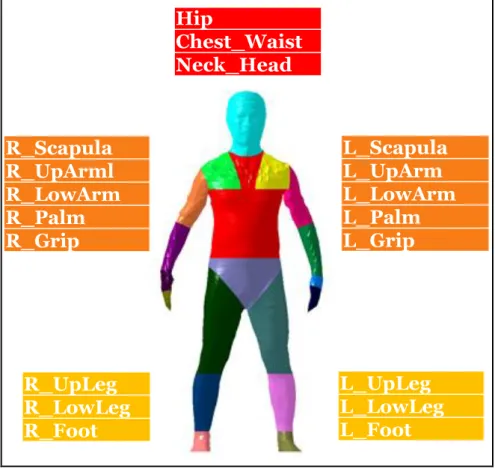
In this study, two kinds of models, Type_0 and Type_2, are introduced, which consist of 19 segments shown in Figure 2.1. The shapes of the segments are constructed based on structural points obtained from optical scans of a human in a static posture [11].

Hip

Chest_Waist Neck_Head

L_Scapula L_UpArm L_LowArm L_Palm L_Grip R_Scapula

R_UpArml R_LowArm R_Palm R_Grip

R_UpLeg R_LowLeg R_Foot

L_UpLeg L_LowLeg L_Foot

Figure 2.1 Segment diagram.

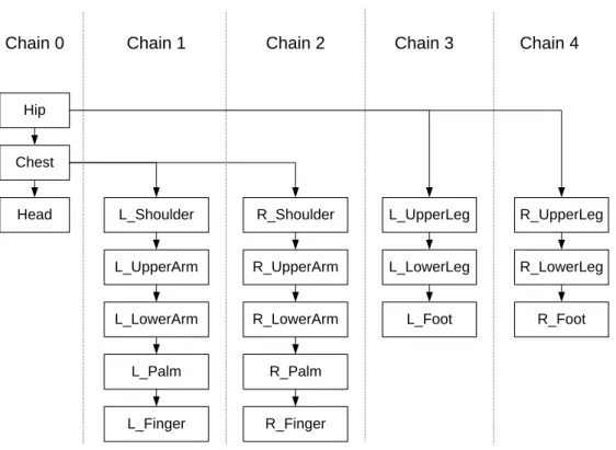
The model is composed of five chains, and each chain contains several links. Its hierarchical structure is shown as Figure 2.2.

(17)

Hip

Chest

Head L_Shoulder

L_UpperArm

L_LowerArm

L_Palm

L_Finger

R_Shoulder

R_UpperArm

R_LowerArm

R_Palm

R_Finger

L_UpperLeg

L_LowerLeg

L_Foot

R_UpperLeg

R_LowerLeg

R_Foot

Chain 0 Chain 1 Chain 2 Chain 3 Chain 4

Figure 2.2 Hierarchical structure chart.

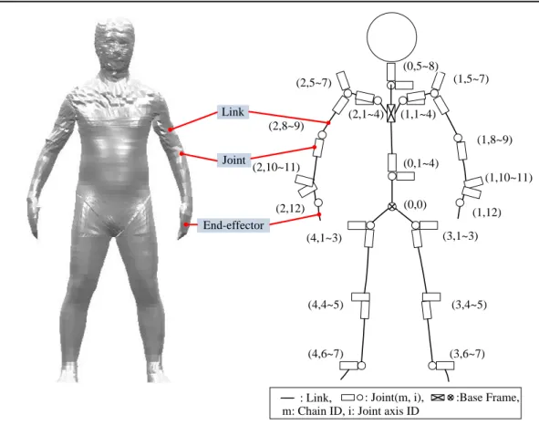
For the Type_0 model, each of the segments has 6 DOF (i.e., forward/backward, up/down, left/right, yaw, pitch, roll), and performs motions based on the Mocap (Motion capture) data. Meanwhile, the Type_2 model has a total of 52 DOF, with the hip serving as the 6-DOF base link. Segments of the human body are viewed as links.

Furthermore, joints connect to links and the last segment of each chain is called end- effector (i.e., head, fingers, feet). The joint and link distribution of the Type_2 model is shown in Figure 2.3, and the DOF of each link is shown in Table 2.1.

(18)

(1,1~4) (2,1~4)

(1,10~11)

: Joint(m, i), :Base Frame, : Link,

(0,0) (0,1~4) (0,5~8)

(1,5~7)

(1,8~9)

(1,12) (2,5~7)

(2,8~9)

(2,12)

(3,1~3)

(3,4~5)

(3,6~7) (4,6~7)

(4,4~5) (4,1~3)

m: Chain ID, i: Joint axis ID (2,10~11)

Link

Joint

End-effector

Figure 2.3 Joint and link distribution diagram of Type_2.

Table 2.1 DOF distribution of Type_2.

Link DOF

Hip 6

Chest_Waist 4

Neck_Head 4

Scapula 4x2

UpArm 3x2

LowArm 2x2

Palm 2x2

Grip 1x2

UpLeg 3x2

LowLeg 2x2

Foot 2x2

The motion of the Type_0 model was based on raw data captured by an optical system for the position and orientation of a set of tracking markers attached to the

(19)

segments of a real human

[12]. At least one reflective marker was placed on each

segment of the subject. Motion data was recorded using an 8-camera D2000 motion capture system at a capture rate of 30 Hz [13]. By contrast, the motion of the Type_2 model was based on changes in the joint angles, where these changes were estimated by means of a two-phase inverse kinematics optimization process, using the Type_0 model as an objective function.

2.2 Introduction of Multi-coordinate Systems

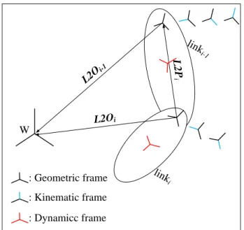
In this section, three coordinate systems, geometric frame, kinematic frame, and dynamic frame are introduced. The geometric frame of the link is defined to display link shape while the segment is formed in structure process. One link only has one geometric frame, while L2O (link to origin) represents the transformation of the geometric frame with respect to the world coordinate shown in Figure 2.4.

Furthermore, L2P (link to previous link) records the transformation of the i^th link with respect to (i-1)^thlink.

W

L2Oⁱ

L2

iP linki-1

link_i L2O^i-1

: Geometric frame : Kinematic frame : Dynamicc frame

Figure 2.4 Multi-coordinate systems.

(20)

For the kinematic frame system, one link can have several kinematic frames with accordance to how many DOF in the link. In addition, the rotation or translation in the z-axis of the kinematic frame is defined as a joint variable. The Type_2 model changes postures according to joint variables.

To construct the dynamic frame system, dynamic parameters must be calculated.

One link only has one dynamic frame. The centroid of the link is defined as the origin of the dynamic frame. Furthermore, the principal axes of the moment of inertia of the link are defined as three directional components.

2.3 Geometric Parameters of Links

The geometric parameters of body segments include the masses, centroids, moments of inertia, etc. The term, geometric parameters, is used in this study because the mass of each human link is the multiplication of volume, which is calculated from the geometric shape of each human link and density, which is referenced from book

[14].

Before proceeding to calculate the geometric parameters, the following methods are used to close the open sections of each segment to avoid omission of the volume calculation. Triangular meshes are used to fill individual body segments. There are two cases of open sections: the structure points of the open section are located at the same girth, or not.

The first case is shown in Figure 2.5. The open sections are located at the first and last girths of this link. An auxiliary point Pc can be added on the open section and build triangular meshes to close it. Equation (2-1) shows the construction of the auxiliary point Pc.

(21)

Auxiliary Point P

c

Figure 2.5 The construction of the auxiliary point Pc.

N i i C

P



 N

(2-1)

where Pi is the 3D point at the girth where we want to construct the auxiliary point, and N is the number of the points at the girth.

Figure 2.6 shows the second case of an open section. In the hip link, the structure points of the side open sections are not locating at the same girth. The closing strategy for side open section is as follows: find the structure points of the open section and use Equation (2-2) to close the open section.

N j j

P



 N

(2-2) Pj is the structure point at the open section which we want to construct the auxiliary point P, and N is the number of the points at the open section.

(22)

There are two open sections through different girths in the hip segment. In Figure 2.6, the open section plots are located at the left and right sides of the hip segment.

The two blue circles represent the connections of the structure points in edges of the hips. The left and right views in Figure 2.6 illustrate the sequences of point indexes, which are also listed in Table 2.2. A two dimension array based on image coding is employed to index the segment’s points, so that each point could be picked according to its indexes [5], The first index represents in which girth the point lies, while the second index corresponds to the point order in a girth. In the left view, the point [0][31]

is set as a start point, and the point [0][43] is set as a final point. In left view, the point [0][6] is set as a start point, and the point [0][18] is set as a final point.

c

[0][6]

[0][11]

[1][7]

[13][19]

[14][20]

[13][20]

[1][8]

[0][14]

[0][31]

[0][36]

[0][39]

[1][33]

[1][34]

[13][59]

[13][58]

[14][60]

Left view Right view

Figure 2.6 Hip segment.

Table 2.2 Point indexes of connecting open sections of hip segment.

(23)

Left view Right view [0][31]

[0][32]

[0][33]

[0][34]

[0][35]

[0][36]

[1][23]

[2][26]

[3][29]

[4][32]

[5][35]

[6][38]

[7][41]

[8][44]

[9][47]

[10][50]

[11][53]

[12][56]

[13][59]

[14][60]

[13][58]

[12][55]

[11][52]

[10][49]

[9][46]

[8][43]

[7][40]

[6][37]

[5][34]

[4][31]

[3][28]

[2][25]

[1][22]

[0][39]

[0][40]

[0][41]

[0][42]

[0][43]

[0][6]

[0][7]

[0][8]

[0][9]

[0][10]

[0][11]

[1][7]

[2][8]

[3][9]

[4][10]

[5][11]

[6][12]

[7][13]

[8][14]

[9][15]

[10][16]

[11][17]

[12][18]

[13][19]

[14][20]

[13][20]

[12][19]

[11][18]

[10][17]

[9][16]

[8][15]

[7][14]

[6][13]

[5][12]

[4][11]

[3][10]

[2][9]

[1][8]

[0][14]

[0][15]

[0][16]

[0][17]

[0][18]

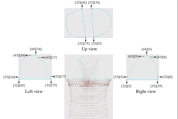
There are four open sections in the chest_waist segment. Two sections are sliced

(24)

through at different girths, and the other two belong to the same girth shown in Figure 2.7. In left and right sides of the chest, the open sections are sliced through at different girths. The closed left section starts at the point [32][75] and ends at the point [32][45], while the left side closing section starts at point [32][35] and ends at point [32][5].

The sequences of points are listed in Table 3. The remaining two open sections in the same girth are easy to arrange, because their point indexes are continuous. Thus, the sequence of points in the left side are [32][45~75], and the sequence of points in the right side are [32][5~35].

[32][5]

[32][75]

[32][35]

[32][45]

[32][5] [32][35]

[33][5]

[43][5]

[44][5]

[43][6]

[33][6]

[32][45] [32][75]

[33][16] [33][17]

[43][16]

[43][17]

[44][16] Up view

Figure 2.7 Chest_waist segment.

Table 2.3 Point indexes of connecting open sections of chest_waist segment.

(25)

Left view Right view [32][75]

[33][17]

[34][17]

[35][17]

[36][17]

[37][17]

[38][17]

[39][17]

[40][17]

[41][17]

[42][17]

[43][17]

[44][16]

[43][16]

[42][16]

[41][16]

[40][16]

[39][16]

[38][16]

[37][16]

[36][16]

[35][16]

[34][16]

[33][16]

[32][45]

[32][35]

[33][6]

[34][6]

[35][6]

[36][6]

[37][6]

[38][6]

[39][6]

[40][6]

[41][6]

[42][6]

[43][6]

[44][5]

[43][5]

[42][5]

[41][5]

[40][5]

[39][5]

[38][5]

[37][5]

[36][5]

[35][5]

[34][5]

[33][5]

[32][5]

There are two armholes in the left and right shoulders as shown in Figure 2.8 and

(26)

Figure 2.9. In left armhole of left shoulder, the start point is [0][0], and the end point is [0][30], as listed in Table 2.4. In right armhole, the start point is [0][12], and the final point is [1][11], as listed in Table 2.5.

[0][12] [0][18]

[1][12]

[2][11]

[7][11]

[6][10]

[2][10]

[1][11]

[0][0]

[1][23]

[0][30]

[12][0]

[2][21]

[11][21]

Right view Left view

Figure 2.8 Left shoulder segment.

Table 2.4 Point indexes of connecting open sections of left shoulder segment.

[0][0]

[1][0]

[2][0]

[3][0]

[4][0]

[5][0]

[6][0]

[7][0]

[8][0]

[9][0]

[10][0]

[11][0]

[12][0]

[11][21]

[10][21]

[9][21]

[8][21]

[7][21]

[6][21]

[5][21]

[4][21]

[3][21]

[2][21]

[1][23]

[0][30]

[0][12]

[0][13]

[0][14]

[0][15]

[0][16]

[0][17]

[0][18]

[1][12]

[2][11]

[3][11]

[4][11]

[5][11]

[6][11]

[7][11]

[1][10]

[1][11]

For the right shoulder, the closing method is similar to that of the left shoulder. In

(27)

left view of the right shoulder, the start point is [0][12], and the end point is [1][11].

In right view, the start point is [0][12], and the final point is [1][11]. The structure points in both shoulders are symmetric, so the point indexes of the connecting open sections can be interchanged as well.

[0][0]

[12][0]

[1][23]

[0][30]

[2][21]

[11][21]

[0][12] [0][18]

[1][12]

[2][11]

[7][11]

[6][10]

[2][10]

[1][11]

Right view Left view

Figure 2.9 Right shoulder segment.

Table 2.5 Point indexes of connecting open sections of right shoulder segment.

[0][12]

[0][13]

[0][14]

[0][15]

[0][16]

[0][17]

[0][18]

[1][12]

[2][11]

[3][11]

[4][11]

[5][11]

[6][11]

[7][11]

[6][10]

[5][10]

[4][10]

[3][10]

[2][10]

[1][11]

[0][0]

[1][0]

[2][0]

[3][0]

[4][0]

[5][0]

[6][0]

[7][0]

[8][0]

[9][0]

[10][0]

[11][0]

[12][0]

[11][21]

[10][21]

[9][21]

[8][21]

[7][21]

[6][21]

[5][21]

[4][21]

[3][21]

[2][21]

[1][23]

[0][30]

The algorithm Lee

[16] developed is employed to calculate the geometric

parameters of body segments after closing up the open sections of each segment.

(28)

Chapter 3. Two-Phases Inverse Kinematics

Relationships between the links in the Type_2 model are modeled using D&H notation [17]. In the Type_0 model, 6 DOFs exist between adjacent links. However, in the Type_2 model, the jointed links have less than 4 DOF. Thus, they have an insufficient number of DOFs to replicate the posture of the Type_0 model directly.

Therefore, an inverse kinematics optimization procedure is performed to determine the appropriate joint angles. In the first step, an optimization method is used to obtain an initial fit of the joint angles for the Type_2 model calculated from the optical motion data. In the second step, the end-effector positions are adjusted iteratively such that the pose of the Type_2 model approaches that of the Type_0 model.

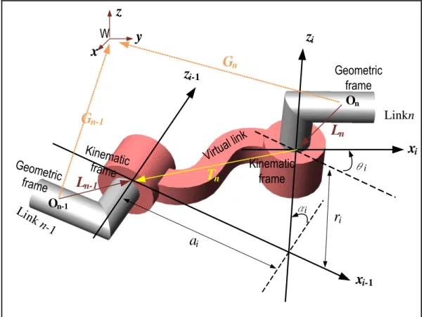
3.1 Forward Kinematics

According to the D&H conventions, the relationship between two pair-axes can be completely defined by four parameters: [



_i,

a ,

_i



_i,

r ], where

_i



_i is the twist angle of axis i,

a is the link length,

_i

r is the offset, and

_i



_i is the rotating angle of the axis. A transformation Ki from the frame of axis i to that of axis i-1 can be written as

[

18

]:

0 0 0 0 1

i i i

i i i i i i i

Cos Sin a

Sin Cos Cos Cos Sin r Sin Sin Sin Cos Sin Cos r Cos

 

     

  

   

 

  

 

 

K

i (3.1)

(29)

z

i-1

z

i

Link n

Lin k n- 1

x

i-1

x

i

α

i

a

i

r

i

x

y z

G

n

G

n-1

T

n

L

n

L

n-1

O

n

O

n-1

Virt ual link Geometric frame

W

Kinematic frame

Geometric frame

Kinematic frame

i

θ

Figure 3.1 D&H parameters of a two-freedom joint between two adjacent links.

For a kinematic chain in the Type_2 model, there are fn pair-axes between link n and n-1, as shown in Figure 3.1. The transformation matrix Tn across all the axes between links n and n-1 is given by

13 14

11 12

23 24

21 22

1 31 32 33 34

0 0 0 1

n

i

i f

t t t t

 

 

 

 

 

 



n i

T K

(3.2)

3.2 The 1

^st

Phase Inverse Kinematics

The 1st-phase of the IK optimization method can be formulated as follows:

(30)

 

' '

13 14

11 12

' '

1 1 21 22 23 24

' ' '

1 1 ' ' ' '

31 32 33 34

0 0 0 1

n n n n n

t t t t

 

 

 

 

    

 

 

T L G G L

, (3.3)

where the superscript [′] denotes the coordinates obtained from the optical system, while G

'

_n and G

'

_n-1 are the transformations of links n and n-1, respectively, with respect to the world frame as shown in Figure 3.1. Furthermore, Ln and Ln-1 are the transformations from the kinematic frames of links n and n-1, respectively, to the geometric frames. In practice, T

'

n is a transformation matrix which requires a 6-DOF joint to reproduce the related motion. However, as described above, the joints between adjacent links in the Type_2 model have less than 4 DOF, and are therefore unable to match the required poses.

In the present study, the Newton method and Fletcher-Reeves method [19] are used to optimize the joint variables such that the position of the links in the Type_2 model approximate those in the Type_0 model to the greatest extent possible. More specifically, the discrepancy between the transformation matrices, Tn, computed from the first stage of the IK optimization process and those derived from the raw data, T

'

n, are minimized so as to satisfy the following equation:

∆E = min[Tn

- T '

n]. (3.4)

(31)

3.2.1 One Degree of Freedom

In 1-DOF joint case, the transformation matrix of a 1-DOF joint is written as:

 

   

13 14

11 1 12 1

23 24

21 1 22 1

1 1

33 34

31 1 32 1

0 1

0 0

t t

 

  

 

 

  

 

 





Tn K . (3.5)

The translation components of the matrix are all constants, and so the only variable available for optimization is the rotation angle θ1 in the orientation. The objective function in Eq. (3.6), for the orientation error R(θ1) based on Eq. (3.4), is designed as the dot product of the component vectors in Eq. (3.5):

 

     

 

     

 

1

2 2

' ' '

11 1 11 21 1 21 31 1 31

' ' ' 2

1 12 1 12 22 1 22 32 1 32

' ' ' 2

13 13 23 23 33 33

1 1 1

t t t t t t

R t t t t t t

t t t t t t

  

   

     

 

     

 

   

 





. (3.6)

Finally the Fletcher-Reeves optimization method is used to solve the above expression.

3.2.2 Two Degree of Freedom

The transformation matrix of a 2-DOF joint is given by

 

   

       

   

       

11 1 2 12 1 2 13 1 14 1

21 1 2 22 1 2 23 1 24 1

1 2 1 2

31 1 2 32 1 2 33 1 34 1

, ,

, , ,

0 0 0 1

t t t t

     

       

 

 

   

 

 

Tn K K , (3.7)

(32)

where

14 2 1 2 1 2 1

24 2 1 1 2 1 2 2 2 1 2 1 1

34 2 1 1 2 1 1 2 2 1 2 1 1

cos sin sin

sin cos cos sin cos sin cos sin sin sin cos sin sin cos cos cos

t a r a

t a r r r

  

       

  

   

   

In an inverse kinemics process, the position error is more important than the orientation error. Therefore, the variables in a traslation component have a high priority to be solved in general cases. There are two cases for solving θ1. In the first case, the origins of two kinematic frames are not coincident. An object function to minimize the position error P(θ1) is defined by Eq. (3.8). In the other case, a objective function for θ1 must be set as Eq. (3.9) to minimize the differences of w-components of link orientations, since the offset parameter a2 and the slide parameter r2 both are zero. Notice that t14 = a1, t24 = -r1 sinα1

and t

34 = -r1 cosα1, while the origins of two kinematic frames are coincident. Eq. (3.8) is useless for solving θ1 due to the translation component always being constant and not truely a function of θ1. Thus, Eq. (3.9) is used to solve θ1.

 ¹



¹⁴ ¹ ¹⁴^'



²



²⁴^{ }¹ ²⁴^'



²



³⁴^{ }¹ ³⁴^'



² ¹²

P  ^ t  t  t  t  t  t ^ (3.8)

 

1



13 13^'

 

² 23 23^'

 

² 33 33^'



²

R



 t t  t t  t t (3.9)

Newton’s method is used to optimize θ1. The rotational part in Eq. (3.7) is reduced to a single variable problem after obtaining joint angle θ1. And then, the same process as Eq. (3.9) is applied again to get θ2.

(33)

3.2.3 Three Degree of Freedom

The transformation matrix of a 3-DOF joint is written as:

 

   

       

   

       

11 1 2 3 12 1 2 3 13 1 2 14 1 2

21 1 2 3 22 1 2 3 23 1 2 24 1 2

1 2 3 1 2 3

31 1 2 3 32 1 2 3 33 1 2 34 1 2

, , , , , ,

, ,

, , , , , ,

0 0 0 1

t t t t

         

  

         

 

 

   

 

 

Tn K K K (3.10)

The orientation parts in the matrix have three variables θ1,

θ

2 and

θ

3, while the translation parts have two variables θ1 and

θ

2. The objective function for position error

P(θ

1, θ2) is given by



¹^, ²

 

¹⁴



¹^, ²



¹⁴^'



²



²⁴

^

¹^, ²

^

²⁴^'



²



³⁴

^

¹^, ²

^

³⁴^'



² ¹²

P

 

^ t

 

t  t

 

t  t

 

t ^ . (3.11)

The objective function for the orientation error R(θ1, θ2, θ3) which is dot product of vectors, is given by

 

     

 

     

 

     

 

1

2 2

' ' '

11 1 2 3 11 21 1 2 3 21 31 1 2 3 31

' ' ' 2

1 2 3 12 1 2 3 12 22 1 2 3 22 32 1 2 3 32

' ' ' 2

13 1 2 13 23 1 2 23 33 1 2 33

, , , , , , 1

, , , , , , , , 1

, , , 1

t t t t t t

R t t t t t t

t t t t t t

        

           

     

    

 

    

 



 

 

 

(3.12)

If the origins of the third and the second kinematic frames are coincident, a redundant problem will occur. Once θ1 becomes the best value in Eq. (3.11), P(θ1, θ2) will always have the same error value no matter how θ2 changes. Thus, variables θ1

and θ2 can not be solved in accordance with the translation part. It should be given priority to decrease the orientation error, so as to be directly solved in Eq. (3.12).

(34)

Finally, Fletcher-Reeves method is used to solve this multivariable problem.

3.2.4 Four Degree of Freedom

The transformation matrix of a 4-DOF joint, between two adjacent links, can be given as

 

   

       

   

       

11 1 2 3 12 1 2 3 13 1 2 14 1 2 4

21 1 2 3 22 1 2 3 23 1 2 24 1 2 4

1 2 3 4 1 2 3 4

31 1 2 3 32 1 2 3 33 1 2 34 1 2 4

, , , , , , ,

, , ,

, , , , , , ,

0 0 0 1

t t t t r

r t t t t r

         

  

         

 

 

   

 

 

Tn K K K K . (3.13)

K

4 is the transformation matrix of the prismatic axis, and r4 is a variable. The orientation component has three variables θ1, θ2 and θ3, while translation has variables

θ

1, θ2 and r4. The objective function for position error P(θ1, θ2, r4) is given by

 



 

 

 

 

 



1

2 2 2 2

' ' '

1, 2, 4 14 1, 2, 4 14 24 1, 2, 4 24 34 1, 2, 4 34

P   r ^ t   r t  t   r t  t   r t ^ . (3.14)

The objective function for the orientation error is the same as Eq. (3.13). For a 4- DOF joint, since the prismatic axis lies along the direction toward the next link, the orientation part must be solved first. After obtaining orientaion variables θ1, θ2 and

θ

3, the variable r4 can be solved by Eq. (3.14). The Fletcher-Reeves method is used to produce optimized solutions.

3.3 The 2

^nd

Phase Inverse Kinematics

In the 2^nd phase of IK, there are two procedures to make end-effectors of the Type_2

(35)

model reach targets, end-effectors of the Type_0 model. The 2^nd phase IK takes the whole kinematic chain into account rather than just the adjacent links. The aim of the optimization procedures is to solve the joint variables in such a way that the end- effector of each chain is placed in a specific location. Note that the initial guess of the joint variables is set in accordance with the results obtained in the first phase of the IK optimization process.

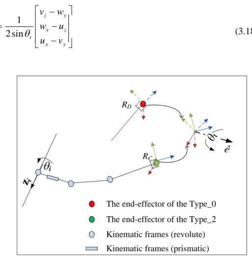
At the first procedure, the axis-angle method

[20] is used to estimate how many

degrees each joint axis zi should move by Eq. (3.15) to make orientations of the end- effectors of the Type_2 model approach orientations of the targets.

A rotation transformation RT means a desired orientation RD with respect to a current orientation RC as Eq. (3.16). In Figure 3.2, θt represents how many degrees the end-effector of the Type_2 should move according to the rotation axis ê, which is calculated by the axis-angle method. Accordingly, the matrix RT is converted to axis- angle by Eqs. (3.17) and (3.18). Since joint axis zi and the ideal rotation axis ê are not coaxial, the angle θi which joint axis zi moves should equal to θt multiply a dot product with joint axis zi and rotation axis ê. This procedure is complete if all joints renew once.

θ

i = θt * (ȇ ∙ zi) (3.15)

    

T D C ¹ ^xy ^xy ^xy

z z z

u v w

R R R u v w

u v w



 

 

   

 

 

(3.16)

1 1

cos [ ]

2

x y z

t

u v w



 ^ ^ ^ ^ (3.17)

(36)

ˆ 1

2 sin

z y

x z

t

x y

v w

e w u

u v



  

 

   

  

 

(3.18)

z

ⁱ

The end-effector of the Type_0 The end-effector of the Type_2 Kinematic frames (revolute) Kinematic frames (prismatic)



^t

ê



i

R

D

R

C

Figure 3.2 Axis-angle method to approach a target.

The second procedure is based on the CCD (Cyclic Coordinate Descent) method

[21] for a chain with N joints between the chain base and the end-effector, the

optimization process consists of N steps per iteration. In performing the optimization procedure, only the i^th variable is changed in the i^th step. The posture of the end- effector is then updated accordingly.

In optimizing the joint angles, the objective function is specified as the error E^* between the Type_2 model and the captured data (i.e. the Type_0 model), as shown in Eq. (3.19). Note that “e” denotes the end-effector, while we and wn are the weighting factors of the end-effector and inboard links, respectively. As shown in Eq.

(3.20), the summation of the weighting factors is equal to unity. Furthermore, “En” in

(37)

Eq. (3.19) represents the total error of the n^th link and is defined in Eq. (3.21). As shown in computing the error, the angles in the orientation part are multiplied by the link length ln and added to the position error of the frame origin dn.

* 1 e

n n n

E w E





^, ^(3.19)

1

e n n

w



 

^, ^(3.20)

2 2 2

n n x y z n

E  l       d

, (3.21)

' 1

cos ^k ^k' , , ,

k

k k

V V k x y z V V

 ^ ^^_ ^^_

 

 

 

 (3.22)

The angle φk between the two unit vectors is given by Eq. (3.22). Let Vk be the unit vectors in the x-, y-, and z-axes for the n^th link of the Type_2 model, and V’k be the corresponding unit vectors of the Type_0 model.

3.4 Error Analysis

In Figures 3.3 ~ 3.5, models in right side are Type_2, and models in left side are Type_0. During IK processes, the weighting factor of the end-effector is set to 1. In

(38)

every process, postures of the Type_2 models are always according to the posture of the Type_0 model. Figure 3.3 shows the 1^st phase IK result of the Type_2 model, which errors are listed in Table 3.1.

Figure 3.3 1^st phase IK result.

Table 3.1 Errors of 1^st phase IK result

End-effector Orientation error Position error Total error

Head 41.804 1.65713 43.4611

Left hand 175.098 109.412 284.51

Right hand 87.2219 135.945 223.167

Left foot 20.0985 83.6125 103.711

Right foot 67.8721 37.8328 105.705

(unit: mm )

The result of the axis-angle method in 2^nd phase IK is shown in Figure 3.4. Plots in Tables 3.2 ~ 3.6 show error trends of all end-effectors. In the plots recording orientation errors, all error trends show orientation errors decrease along with loop counts. It is seen that the axis-angle method can improve orientation accuracies of

(39)

end-effectors. The last total errors of all end-effectors are less than the beginnings although some position errors rise. According to Figure 3.3 and Figure 3.4, the orientations of the end-effectors of the Type_2 model replicate the orientations of the end-effectors of the Type_0 model truly better after using the axis-angle method.

Figure 3.4 The result after adjusting the joints using the axis-angle method.

Table 3.2 Error trends of the head based on the axis-angle method

(40)

last orientation error is 0.047 mm after 8 loops

last position error is 42.786 mm after 8 loops

last total error is 42.833 mm after 8 loops

Table 3.3 Error trends of the left hand based on the axis-angle method

(41)

Table 3.4 Error trends of the right hand based on the axis-angle method

(42)

Table 3.5 Error trends of the left foot based on the axis-angle method

(43)

Table 3.6 Error trends of the right foot based on the axis-angle method

(44)

The result of the CCD procedure in 2^nd phase IK is shown in Figure 3.5. In

(45)

performing the CCD procedure, the criterions are set as follows: (1) accuracy 2 mm, (2) loop limit 100 counts, and (3) continuous two error differences not over 0.001 mm. Tables 3.7 ~ 3.11 show error trends of all end-effectors during the CCD procedure. In plots recording position errors, the error trends decrease along with loop counts although there are tiny oscillations in the right foot. During the front section of the CCD procedure, orientation errors almost rise. However, the total errors, orientation errors and position errors all converge stably in the rear section of the CCD procedure. Figure 3.5 shows that the end-effectors of the Type_2 reach the targets with precise orientations and correct positions.

Figure 3.5 The result after applying the CCD method.

Table 3.7 Error trends of the head based on the CCD method

(46)

Table 3.8 Error trends of the left hand based on the CCD method

(47)

Table 3.9 Error trends of the right hand based on the CCD method

(48)

Table 3.10 Error trends of the left foot based on the CCD method

(49)

Table 3.11 Error trends of the right foot based on the CCD method

(50)

Figure 3.6 shows the end-effector error is related to the end-effector weighting at

(51)

the CCD procedure for the case of the left hand. The criterions are set as follows: (1) accuracy 0.01 mm, and (2) loop limit 10000 counts. Note that we is the end-effector weighting and wi is the weighting of each link in the left hand. There are a total of five links in the left hand, and the sum of all the link weightings is equal to 1. It is seen that as we increases, the end-effector error is reduced.

After 1^st stage wi = 0.2 we =0.2 E_e = 191.354

w_i= 0.15 w_e= 0.4 Ee = 182.873

w_i= 0.1 we =0.6 E_e = 15.8123

w_i= 0.0 we = 1.0 E_e = 0.00959733

Table 3.12 2^nd stage IK with different weighting factors.

(52)

Chapter 4. Calculation of Whole Body Dynamics

This chapter proposes a method for determining the dynamic parameters of human motion using a 3D whole human body model. The geometric parameters of the whole body are derived by integrating the geometric parameters of the constitutive links. In addition, the dynamic parameters of the whole body are calculated by deriving the time variant of the dynamic frame defined by the geometric parameters. Finally, a new approach based on the screw method is presented for tracking the ZMP of the human body during motion. The validity of the proposed approach is demonstrated by evaluating the whole body dynamics over the course of a 25-second sequence of continuous moves and postures.

4.1 Geometric Parameters of Whole body

To calculate the geometric parameters of the whole body, it is necessary to integrate the geometric parameters of each link in the model. The geometric parameters of each link are obtained using the algorithm developed by Lee [22]. In this section, the method to compute the geometric parameters of the whole body will be derived.

4.1.1 Mass and centroid

The mass of the whole body M is computed by summing the masses of all the links, as shown in Eq. (4.1), in which mi represents the mass of the i^th link. Finally, the centroid of the whole body, G, is calculated as shown in Eq. (4.2). Note that the centroid G is nominated as the origin of the dynamic frame of the whole body, and pi

is the centroid of the i^th link.

(53)

1 n

i i

m M



 

, (4.1)

1 n

i i

G i

M

p m

 



. (4.2)

4.1.2 Principal Axes of Inertia

The principal axes of the whole body are determined from Eq. (4.3) in accordance with matrix transformation theory and the parallel theorem [23]. Note that Ri is the rotation of the i^th link with respect to the world coordinate frame, Ii is the principal MOI of the i^th link, and di is the skew symmetric matrix associated with the relative position vector (xi, yi, zi). The principal moments of inertia, Ix, Iy and Iz, are eigenvalues of ICoM, while the eigenvectors of ICoM form the orientation of the dynamic frame of the whole body.

[I_CoM]



[R_i][ ][I_i R_i]^T m d_i[ ]_i 2^, ^(4.3)

0

[ ] 0

0

i i

i i i

i i

z y

d z x

y x

  

 

  

 

 

. (4.4)

全身人體運動力學之靜不定問題探討

科技部補助專題研究計畫成果報告 期末報告