煙霧偵測上的時空分析

(1)

國立交通大學

電機與控制工程學系

碩士論文

煙霧偵測上的時空分析

Spatio-Temporal Analysis in Smoke Detection

研究生：李鎮宇

指導教授：林進燈博士

(2)

煙霧偵測上的時空分析

Spatio-Temporal Analysis in Smoke Detection

研究生：李鎮宇 Student：Chen-Yu Lee

指導教授：林進燈博士

Advisor：Dr. Chin-Teng Lin

國立交通大學

電機與控制工程學系

碩士論文

A Thesis

Submitted to Department of Electrical and Control Engineering

College of Engineering and Computer Science

National Chiao Tung University

in Partial Fulfillment of the Requirements

for the Degree of Master

in

Electrical and Control Engineering

June 2009

Hsinchu, Taiwan, Republic of China

(3)

煙霧偵測上的時空分析

學生：李鎮宇

指導教授：林進燈博士

國立交通大學電機與控制工程研究所

Chinese Abstract

摘要

近年來，基於影像式的煙霧偵測技術在智慧型監控系統中受到廣泛的重視與研究。然而，在給定一個廣大的開放空間中來處理煙霧事件與其他的常見的干擾物例如行人和車輛，建立一個穩定且有效率的煙霧偵測系統仍難是一個困難且具有挑戰性的問題。在本篇論文中，我們提出了一個創新與可靠的自動化煙霧偵測架構。本篇論文提出三種重要的特徵：邊緣模糊化、能量的逐步變化與色彩結構的逐步變化。接下來，在考量實際火災與煙霧事件的影片與資料的稀少性下，為了獲得更佳的一般性，我們採用基於支持向量機(Support Vector Machines)的分類器將三種特徵結合。此系統在各種環境與干擾下執行超過六小時以上，並且證明在實際防災應用上的穩健性與可靠性。

本篇論文的目標是在時間域與空間域上分析煙霧的特性，由此系統所得到的實驗結果將可以提供煙霧偵測領域上更深入的理解，並且有助於處理高誤判率和較長的反應時間等問題。

(4)

Spatio-Temporal Analysis in Smoke Detection

Student: Chen-Yu Lee

Advisor: Dr. Chin-Teng Lin

Department of Electrical and Control Engineering

National Chiao Tung University

English Abstract

ABSTRACT

Visual-based smoke detection techniques in surveillance systems have been studied for years. However, given an image in open or large spaces with typical smoke and disturbances of commonly moving objects such as pedestrians or vehicles, robust and efficient smoke detection is still a challenging problem. In this paper, we present a novel and reliable framework for automatic smoke detection. It exploits three features: edge blurring, the gradual change of energy and the gradual change of chromatic configuration. In order to gain proper generalization ability with respect to sparse training samples, the three features are combined using a support vector machine based classifier. This system has been run more than 6 hours in various conditions to verify the reliability of fire safety in the real world.

The objective of this paper is to analyze the characteristic of smoke in spatial and temporal domains. The results obtained from this novel approach would provide better insight to operators in the field of smoke detection to handle the problems of high false alarm rate and long reaction time.

(5)

Chinese Acknowledgements

致

謝

本論文的完成，首先要感謝指導教授林進燈博士這兩年來的悉心指導，讓我學習到許多寶貴的知識，在學業及研究方法上也受益良多。另外也要感謝口試委員們的建議與指教，使得本論文更為完整。其次，感謝超視覺實驗室的大家長鶴章，還有剛維、建霆、肇廷及東霖學長、提供許多寶貴的意見與耐心的指導。宣輯、哲銓及耿為同學的相互砥礪，及所有學長、學弟們在研究過程中所給我的鼓勵與協助。尤其是肇廷學長，在理論及程式技巧上給予我相當多的幫助與建議，讓我獲益良多。感謝我的父母親對我的教育與栽培，並給予我精神及物質上的一切支援，使我能安心地致力於學業。此外也非常感謝妹妹欣潔與女友苑如對我不斷的關心與鼓勵。謹以本論文獻給我的家人女友及所有關心我的師長與朋友們。

(6)

List of Tables

Table 4-1 Properties of the testing videos ... 44

Table 4-2 Experimental results without ADU based on single frame ... 45

Table 4-3 Experimental results with ADU based on single frame ... 46

(9)

List of Figures

Fig. 1-1 Processing diagram of fire development... 1

Fig. 1-2 Four categories of video smoke detection ... 2

Fig. 2-1 System overview ... 5

Fig. 3-1 Block processing ... 6

Fig. 3-2 GMM background model construction ... 7

Fig. 3-3 Background image construction by GMM ... 9

Fig. 3-4 Foreground image obtained by background subtraction ... 9

Fig. 3-5 Smoke regions come into existence and disappear continuously ... 10

Fig. 3-6 Results of block processing ... 11

Fig. 3-7 Horizontal wavelet transform ... 12

Fig. 3-8 Vertical wavelet transform ... 13

Fig. 3-9 Original image and its single level wavelet subimages ... 14

Fig. 3-10 Two-dimension wavelet transform and its coefficients ... 15

Fig. 3-11 Blurring in the edges is visible by single level wavelet subimages ... 16

Fig. 3-12 Demonstration of (a) a Wave and (b) a Wavelet ... 17

Fig. 3-13 Block diagram of 1-D DWT ... 18

Fig. 3-14 Comparison of changes in value of energy ratio at the passage of ... 19

Fig. 3-15 RGB color histogram of a specific block (a) original image (b) covered by ordinary moving objects (c) covered by smoke ... 21

Fig. 3-16 Comparison of changes in value of details in rgb color space at the passage of (a) ordinary moving objects (b) smoke ... 22

Fig. 3-17 Separating hyperplanes ... 24

Fig. 3-18 The optimal separating hyperplane ... 24

Fig. 3-19 Inseparable case in a two-dimensional space ... 27

Fig. 3-20 Transformation of feature space. ... 27

Fig. 3-21 Distribution of the support vectors ... 29

Fig. 3-22 Block-wise output of SVM classifiers ... 29

Fig. 3-23 (a) Arrangement of pixels (b) pixels that are 4-connectivity (c) pixels that are 8-connectivity (d) m-connectivity ... 31

Fig. 3-24 Connected components labeling ... 32

Fig. 3-25 Regard a block as a pixel unit ... 33

Fig. 3-26 Connected blocks labeling ... 33

Fig. 3-27 The adjustment on photo timer ... 34

Fig. 3-28 Alarm decision unit ... 34

Fig. 3-29 System output after alarm decision unit ... 35

(10)

Fig. 4-2 Indoor environment ... 38

Fig. 4-3 Pedestrians ... 39

Fig. 4-4 Outdoor environment with vehicles ... 40

Fig. 4-5 Tunnel environment situations ... 43

Fig. 4-6 The experimental result in [2] ... 47

(11)

1

Chapter 1 Introduction

1.1 Motivation

In last few years, there were average 5622.8 fire accidents per year according to the statistic report from the National Fire Administration. The number of dead and injured people was nearly 700 and the property loss was about 2 billion NT dollars each year. If the fire accident could be found much earlier, it is more likely to reduce the loss of life.

The process of fire development mostly divided into four periods: Ignition, Fire Growth Period, Fully Developed Period and Decay Period as shown in Fig.1-1.

Fig. 1-1 Processing diagram of fire development

In general occurrences of fire, a great quantity of thick smoke instead of fire is produced in the initial stage. After flashover, fire spreads quickly and burns all spaces continuously. If people don’t escape from the scene of a fire before flashover, they

(12)

probably wouldn’t save their life. Therefore, the duration of flashover is the prime time for people to flee from fire.

Conventional point-based smoke and fire detectors typically detect the presence of certain particles generated by smoke and fire by ionization or photometry. An important weakness of point detectors is that in large space, it may take a long time for smoke particles to reach a detector and they can’t be operated in open spaces such as hangers, tunnels, storage, and offshore platform.

Owing to the limitation of the traditional concept, point-based detectors can’t detect fires or smokes in early stage. In recent years, many researches are devoted to video smoke detection that doesn’t rely on proximity of smoke to the detector. This enables it to incorporate standard video surveillance cameras with sophisticated image recognition and processing software to identify the distinctive characteristics of smoke patterns. In most cases, smoke usually appears before ignition. Therefore, the beginning of fire can be observed soon before it causes any real damage.

1.2 Related Work

(13)

There are four categories of video smoke detection in the literature as shown in Fig. 1-2. The first category is Motion-Based approaches. Kopilovic et al. [1] observed that the irregularities in motion due to non-rigidity of smoke. They apply a multiscale optical flow computation and the entropy of the motion distribution in Bayesian classifier to detect the special motion of smoke. In order to save computational time, Yuan [2] proposed a fast orientation model that produces more effective way to extract the motion characteristics. Although significant advances have been made in the development of this work, their adoption in general surveillance systems is not widely reported.

The second one is Appearance-Based approaches. Toreyin et al. [3] indicated that smoke of an uncontrolled fire expands in time which results in regions with convex boundaries. Chen [4] found that airflows will make the shape of smoke to be variously changed at any time. Therefore, a disorder measure, the ratio of circumference to area for the extracted smoke region, is introduced to analyze shape complexity. Growth rate is obtained by increment of smoke pixels due to the diffusion process existed in generation of smoke. Two thresholds are determined by the statistical data of experiments to verify the real smoke; furthermore, the changing unevenness of density distribution is proposed in [5]. The difference image provides a natural way to represent the attribute which has more internal information in smoke frames than non-smoke frames. While much research has been devoted to these techniques, few studies have investigated the situation that smoke and non-smoke objects exist in the same time and the presence of moving objects from the outside of video scenes.

The third one is Color-Based approaches. Smoke usually displays grayish colors during the burning process [4]. Two thresholds of I (intensity) component of HSI color space depend on statistical data and this implies that three components R, G and

(14)

B of the smoke pixel are equal or so. Since smoke color can’t be represented accurately by a single unimodal, the 3D joint probability density function can be decomposed in three marginal unidimensional distributions over each color axis to accommodate different ranges of color [6]. Independent of the fuel type, smoke naturally decreases the chrominance channels U and V values of the candidate region [3]. In spite of the early alarm capability, few experimental results have been conducted in the range of grayish or dull non-smoke objects.

The fourth one is Energy-Based approaches. It is well-known that wavelet coefficients contain the high frequency information of the original image [7]. Since smoke obstructs the texture and edges in the background of an image [3], a decrease in wavelet energy is an important clue for smoke detection. Piccinini et al. [8] further improved the concept by on-line modeling the ratio between the current input frame energy and the background energy. This method performs well in many real cases but needs long reaction time and more exact validation of the input data extracted from surveillance systems that operate 24 hours a day.

1.3 Thesis Organization

The remainder of this thesis is organized as follows. Chapter 2 describes system overview. Chapter 3 shows smoke detection algorithm including background modeling, candidate selection, feature extraction, classification and verification. Chapter 4 shows experimental results and comparisons. Finally, the conclusions of this system and future work will be presented in chapter 5.

(15)

2

Chapter 2 System Overview

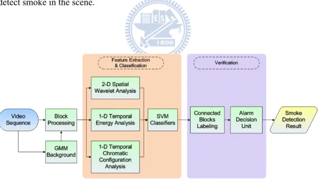
The presented system is an ensemble of different modules as depicted in Fig. 2-1. The main scope of this paper is the feature extraction and classification with respect to candidate region of moving objects.

Foreground segmentation is achieved by using the background suppression approach presented in [9]. After background elimination, foreground is further analyzed to identify moving property. Moreover, feature extraction is processed in candidate regions. The extracted information by the system is further analyzed to detect smoke in the scene.

(16)

3

Chapter 3 Smoke Detection Algorithm

3.1 Block Processing

Figure 3-1 is the flow chart of block processing. The input is the gray level image sequence, and the output is candidate blocks with moving property. There are two common methods for obtaining foreground image. One is temporal difference, the other is background subtraction. Temporal difference method is that we subtract frame

t-1 from frame t, and the regions with a obvious intensity variation are considered as

foreground region. Background subtraction is also in similar way but we use a constructed background image instead of frame t-1.

Generally, cameras are usually set fixedly by considering surveillance monitoring system. Therefore, background subtraction is a better choice for our proposed algorithm. Foreground regions can be found by background subtraction, but they could also include static objects. Next, temporal difference of two successive frames will be calculated. The two methods are combined to further filter out static objects.

(17)

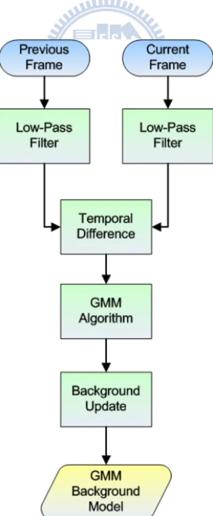
3.1.1 Background Modeling

Gaussian Mixture Model (GMM) [9] is a common and robust method in background construction, and we choose GMM to build the background image. It will be described as follows.

Generally speaking, the intensity of each pixel varies in a small interval except the region of foreground objects. It is proper to use a Gaussian model to construct the background image. But in many surveillance videos, we would observe that there are waving leaves, sparking light, etc. In these situations, some background pixels would vary in several specific intervals. In other words, using two, three or more Gaussian distributions to model a pixel will obtain a better performance. We present the flow chart of GMM background construction in Fig. 3-2.

(18)

Firstly, we use a low-pass filter to reduce the noise. The GMM method models intensity of each pixel with K Gaussian distributions. The probability that a certain pixel has a value of X at time t can be written as. t

K , , , 1

( )

t k t

( ,

t k t

,

k t

)

k

P X

ω

η

X

μ

=

∑

⋅

∑

_(3.1)

where K is the number of distributions that we used,

ω

k t, represents the weight of

k-th Gaussian in the mixture at time t,

μ

k t, is the mean of k-th Gaussian in the

mixture at time t, ∑ is the covariance matrix of the k-th Gaussian in the mixture at k t,

time t, and η is a Gaussian probability density function shown in Eq. (3.2)

( )

/ 2 _{1/ 2} 1 1 1 ( , , ) exp{ ( ) ( )} 2 2 | | T t t t _n t t t t t t X X X η π

μ

_{∑ =} ₋ ₋

μ

_∑ − ₋

μ

∑ (3.2)

where n is the dimension of data. In order to simplify the computation, it assumed that each channel of data are independent and have the same variance, and then can assume the covariance matrix as Eq. (3.3):

2

, I

k t σ_k

∑ = (3.3) Temporal difference is applied to extract the possible background regions, and update pixels inside these regions. Then, we sort Gaussian distributions by the value of ω σ , and choose the first B distributions to be the background model, i.e. shown /

as Eq. (3.4): , 1 arg min( b k t ) b _k B

ω

T = =

∑

> (3.4) When a new pixel is inputted (intensity is Xt+1), it will be checked against the K

distributions by turns. If the probability value is within 2.5 standard deviations, and this pixel is considered as background. Then, we update weight, mean, variance by Eq. (3.5), (3.6), (3.7):

(19)

, 1 (1 ) , ( , 1) k t k t Mk t ω + = −α

ω

+α + (3.5) 1 (1 ) 1 t ρ t ρXt

μ

+ = −

μ

+ + (3.6) 2 2 1 1 1 1 1 (1 ) ( t t ) (T t t ) t t X X σ ₊ = −ρ σ +ρ + −μ + + −μ + (3.7)

where α is a learning rate, Mk t, +1 is 1 for the model which matched and 0 for

remaining models, and Eq. (3.8) shows the second learning rate ρ.

1 , ,

(Xt | k t, k t)

ρ = αη + μ σ (3.8)

Besides, the remaining Gaussians only update the weight. If there is no any distribution is matched, we replace the mean, variance and weight of the last distribution by Xt+1, a high variance and a low weight value, respectively. Figure

3-3 shows the constructed background image by GMM. Figure 3-4 shows the foreground image obtained by background subtraction.

(a) Video sequence (b) GMM Background Image Fig. 3-3 Background image construction by GMM

(a) Current image (b) Foreground image Fig. 3-4 Foreground image obtained by background subtraction

(20)

3.1.2 Candidate Selection

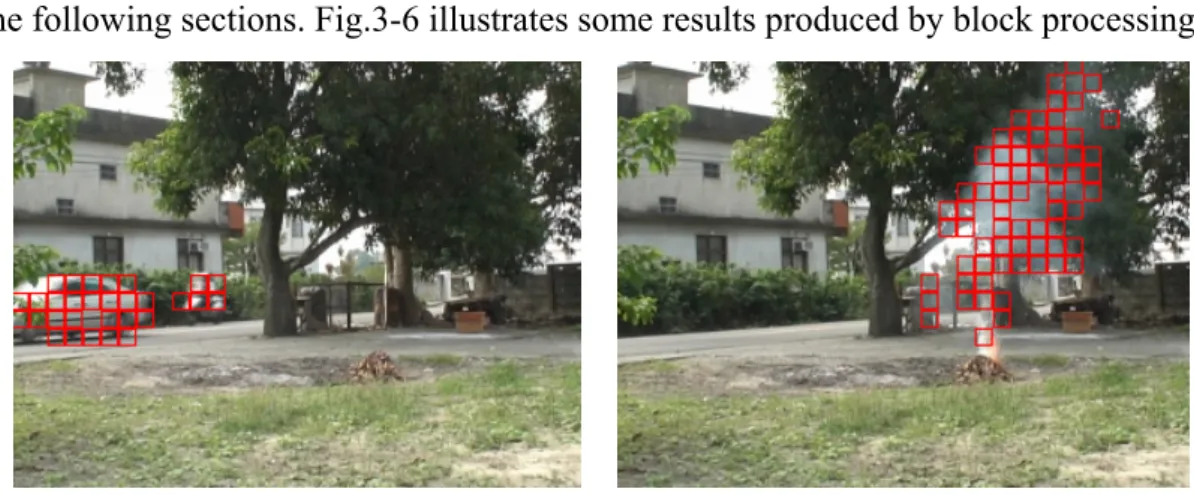
Smoke regions come into existence and disappear continuously because of the special particle property during ignition and combustion as shown in Fig.3-5. It is inefficient to track or analyze the target using object-based method. Block-based technique provides a better way to solve this problem. The image will be divided into non-overlapped blocks, and each block has the same size in a same image. First, we will find out the blocks with a gray-level change. The foreground image will be obtained by the GMM approach, and we compute the summation of foreground image for each block as shown in Eq. (3.9)

(

)

1 , 1, , , 0, k x y S k if foreground x y t T S otherwise ∈ ⎧ ⎡ ⎤ > ⎪ _⎣ _⎦ = ⎨ ⎪ ⎩

∑

_(3.9)

where Sk is the kth block and x,y is the coordinates of the scene. T1 is the predefined

threshold.

(21)

Foreground regions can be found by the GMM approach, but they could also include static objects. Next, temporal difference of two successive frames will be calculated. In dynamic image analysis, all pixels in the difference image with value “1” are considered as moving objects in the scene. As we know, video images usually have a great amount of noises due to intrinsic electronic noises and quantification. So the difference of two successive frames pixel inevitably produces false segmentation. To reduce the disturbance of noises, we also compute its summation for each block to determine the moving property. The block difference is defined as

(

)

(

)

2 , 1, , , , , 0, k x y T k if f x y t f x y t t T T otherwise ∈ ⎧ ⎡ − − Δ ⎤ > ⎪ _⎣ _⎦ = ⎨ ⎪ ⎩

∑

_(3.10)

where Tk is the kth block and x,y is the coordinates of the scene, f is the input image

and T2 is the predefined threshold.

In order to reduce the computational cost, only when the value of background subtraction and temporal difference lager than the predefined thresholds will be regarded as candidates containing moving objects by Eq. (3.11).

1, 1 0, k k k if S AND T B otherwise = ⎧ = ⎨ ⎩ (3.11)

We consider the information of a particular block over time as a “block process” in the following sections. Fig.3-6 illustrates some results produced by block processing.

(22)

3.2 2-D Spatial Wavelet Analysis

Although the Fourier transform has been the mainstay of transform-based image processing since the late 1950s, a more recent transformation, called the wavelet transform, is now making it even easier to compress, transmit, and analyze many images. Unlike the Fourier transform, whose basis functions are sinusoids, wavelet transforms are based on small waves, called wavelets, of varying frequency and limited duration. This allows them to provide the equivalent of a musical score for an image, revealing not only what notes (frequencies) to play but also when to play them. Conventional Fourier transforms, on the other hand, provide only the notes or frequency information; temporal information is lost in the transform process.

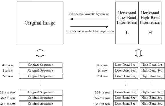
Now we want to transform an image (M by N) into wavelet domain. The whole 2-D spatial wavelet transform can be decomposed by the horizontal wavelet transform and the vertical wavelet transform. Fig. 3-7 is the diagram of horizontal wavelet transform. The direction from left to right is the wavelet decomposition, and the direction from left to right is the wavelet synthesis.

(23)

Each row of the image will be regarded as mutual independent image sequences and each independent row will process wavelet transform respectively. Briefly, a original image will be decomposed into low-band information on the left side and high-band information on the right side after horizontal wavelet transform. We used L and H stand for low-band and high-band information, respectively.

Vertical wavelet transform will process on L and H obtained by horizontal transforms and the whole wavelet transform will be done. Fig. 3-8 is the diagram of vertical wavelet transform. The direction from left to right is the wavelet decomposition, and the direction from right to left is the wavelet synthesis. The data on the left side was processed by horizontal wavelet transform but not vertical wavelet transform yet. Each column of the image will be regarded as mutual independent image sequences and each independent column will process wavelet

(24)

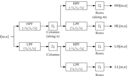
transform, respectively. Anyhow, the data can further separate into upside and underside after vertical wavelet transform. The upside is the vertical low-band information and the underside is the vertical high-band information as shown on the right side of Fig. 3-8. To operate in coordination with horizontal transform, the whole image data can separate into four regions, which are horizontal low-band vertical low-band (LL), horizontal low-band vertical high-band (LH), horizontal high-band vertical low-band (HL), and horizontal high-band vertical high -band (HH).

It is well-known that wavelet subimages contain the texture and edge information of the original image. Edges produce local extreme in wavelet subimages [7]. Wavelet subimages LH, HL, and HH contain horizontal, vertical and diagonal high frequency information of the original image, respectively. Fig. 3-9 is the original image and its single level wavelet subimages.

(25)

Because smoke blurs the texture and edges in the background of an image, high-frequency information becomes much moreinvisiblewhen smoke covers part of the scene. Therefore, details will be an important indicator of smoke due to the decrease in value of high-frequency information. Energy of details is calculated for each candidate block:

(

)

( )

2

( )

2

( )

2 , , , , , k k t x y B E B I LH x y HL x y HH x y ∈ ⎡ ⎤ =

∑

_⎣ + + _⎦ (3.12) where Bk is the kth block of the scene, It is the input image at time t and the wavelet

transform coefficients are shown in Fig. 3-10.

Fig. 3-10 Two-dimension wavelet transform and its coefficients

Instead of using energy of the input directly, we prefer computing the energy ratio of the current frame to the background model due to the cancelation of negative effect on different conditions and the capability of impartial measurement in the decrease:

( )

₍

(

,

)

₎

, k t k k t E B I B E B BG α = (3.13)

where BGt is the mean value of the distribution with a highest weight in the GMM

background model. The value of the energy ratio α is our first feature in spatial domain, which supports the fact that the texture or edges of the scene observed by the

(26)

camera are no longer visible as they used to be in the current input frame. It is also possible to determine the location of smoke using the wavelet subimages as shown in Fig. 3-11.

(a) Original frame without smoke

(b) Frame with smoke

Fig. 3-11 Blurring in the edges is visible by single level wavelet subimages

3.3 1-D Temporal Energy Analysis

A wave is an oscillating function of time or space and is periodic. In contrast, wavelets are localized waves. They have their energy concentrated in time or space and are suited to analysis of transient signals. While wavelet transform and STFT (Short Time Fourier Transform) use waves to analyze signals, the wavelet transform uses wavelets of finite energy (Fig. 3-12). The wavelet analysis is done similar to the STFT analysis. The signal to be analyzed is multiplied with a wavelet function just as it is multiplied with a window function in STFT, and then the transform is computed

(27)

(a) (b) Fig. 3-12 Demonstration of (a) a Wave and (b) a Wavelet

for each segment generated. However, unlike STFT, in wavelet transform, the width of the wavelet function changes with each spectral component. The wavelet transform, at high frequencies, gives good time resolution and poor frequency resolution, while at low frequencies, the wavelet transform gives good frequency resolution and poor time resolution.

Here we only use one level of the transform for fast computation. The 1-D wavelet transform of a signal x is calculated by passing it through a series of filters. First the

samples are passed through a low pass filter with impulse response g resulting in a

convolution of the two:

[ ]

(

)

[ ]

[ ] [

]

k

y n x g n ∞ x k g n k

=−∞

= ∗ =

∑

− (3.14) The signal is also decomposed simultaneously using a high-pass filter h. The outputs

giving the detail coefficients (from the high-pass filter) and approximation coefficients (from the low-pass filter). It is important that the two filters are related to each other and they are known as a quadrature mirror filter.

However, since half the frequencies of the signal have now been removed, half the samples can be discarded according to Nyquist’s rule. The filter outputs are then subsampled by 2.

(28)

[ ]

[ ] [

2

]

low k y n ∞ x k g n k =−∞ =

∑

− (3.15)

[ ]

[ ] [

2 1

]

high k y n ∞ x k h n k =−∞ =

∑

+ − (3.16) This decomposition has halved the time resolution since only half of each filter output characterizes the signal. Each output has half the frequency band of the input so the frequency resolution has been doubled.

Fig. 3-13 Block diagram of 1-D DWT

With the subsampling operator ↓

(

y k n↓

)

[ ] [ ]

=y kn (3.17) the above summation can be written more concisely :

(

)

2 low y = x g∗ ↓ (3.18)

(

)

2 high y = x h∗ ↓ (3.19) Ordinary moving objects such as pedestrians or vehicles have solid characteristic so we can’t see details behind through the bodies. If there is an ordinary moving object going through the candidate block then there will be a sudden energy change because of the transition from the background to the foreground object. On the contrary, initial smoke has semi-transparent nature and becomes less visible as time goes by.

A gradual change of energy is guaranteed to this process and any abrupt variation will be regarded as a noise caused by common disturbance. One-dimension temporal

(29)

wavelet analysis of energy ratio α provides a proper evaluation of this phenomenon. We obtain high-band (details) and low-band (approximations) information by the 1-D DWT shown in Fig.3-13. Therefore, the disturbance can be measured by computing the summation of details for a predefined time interval. Obviously, ordinary solid moving objects produce a great quantity of details in Fig. 3-14(a). Smoke has smooth variation in value of energy ratio and produces few details shown in Fig. 3-14(b). The likelihood of the candidate block to be a smoke region is in inverse proportion to the parameter β

( )

n

[ ]

k D n B n β =

∑

(3.20)

where D[n] is the high-frequency information of energy ratio α and n is the number of time with a non-zero value of details.

(a) (b) Fig. 3-14 Comparison of changes in value of energy ratio at the passage of

(30)

3.4 1-D Temporal Chromatic Configuration Analysis

Smoke can’t be defined by a specific color appearance. However, it is possible to characterize smoke by considering its effect on the color appearance of the region on which it covers. Besides the gradual change of energy, smoke has the same property of color configuration.

Color analysis is performed in order to identify those pixels in the image that respect chromatic properties of smoke. The RGB color space and photometric invariant features are considered in the analysis. Photometric invariant features are functions describing the color configuration of each image coordinate discounting local illumination variations. Hue and saturation in the HSV color space and the normalized-RGB color space are two photometric invariant features in common use. We decided to use the normalized-RGB color space for its fast computation since it can be obtained by dividing the R, G and B coordinates by their total sum. The transfer function is given by

B G R B b B G R G g B G R R r + + = + + = + + = , , (3.21) This transformation projects a color vector in the RGB cube into a point on the unit plane described by r + g + b = 1.

From the empirical analysis, smoke lightens or darkens each component in RGB color space of the covered point but smoke doesn’t severely change the values of the

rgb color system. However, the values are likely to change in case of a material

change. This constrain can be represented by

(

) (

)

(

)

(

)

(

) (

)

, , , , , , , , , k k k r B t r x y t t g B t g x y t t b B t b x y t t ≅ + Δ ≅ + Δ ≅ + Δ (3.22) when the candidate blocks covered by smoke region instead of ordinary moving

(31)

objects. To this end, we draw the RGB color histogram of a specific block in three different situations of a video sequence in order to characterize the presence or absence of smoke. Obviously, the color histogram distribution in Fig. 3-15 (c) is similar to the one in Fig. 3-15 (a). However, the presence of pedestrian produces totally different color histogram distributions between Fig. 3-15 (b) and Fig. 3-15 (a).

(a)

(b)

(c) Fig. 3-15 RGB color histogram of a specific block (a) original image (b) covered by

(32)

The details (high-frequency information) of the three channels in the rgb color

system are obtained by the 1-D DWT again in Fig. 3-13. We can obviously see that ordinary solid moving objects produce a great quantity of details in Fig. 3-16 (a). Smoke has smooth variation in rgb color space and produces few details shown in Fig.

3-16 (b). Therefore, the third feature ρ will be calculated by

( )

(

[ ]

)

2 interval , , max D n D n D n B _r _g _b n k = _∈ ρ (3.23) where Dr[n], Dg[n], and Db[n] stand for details of r, g and b channels respectively and

the value of r, g and b are averages of candidate blocks. Again, the likelihood of the

candidate block to be a smoke region is in inverse proportion to the parameter ρ.

Fig. 3-16 Comparison of changes in value of details in rgb color space at the passage

(33)

3.5 Classification

The difficulty in acquiring smoke or fire accident video should be concerned with practicality. Consequently, the complementary characteristic of the three features extracted from candidate blocks must be learned by a powerful classification model with robust generalization ability.

Support Vector Machines (SVMs) have considerable potential as classifiers of sparse training data which are developed to solve the classification and regression problems. SVMs have similar roots with neural networks, and it demonstrates the well-known ability of being universal approximates of any multivariable function to any desired degree of accuracy. This approach is produced by Vapnik et al. using some statistical learning theory [10][12][13].

3.5.1 Support Vector Machines

Hard-Margin Support Vector Machines

SVM is a way which starts with a linear separable problem. First, we discuss hard-margin SVMs, in which training data are linearly separable in the input space. Then we extend it to the case where training data cannot be linearly separable.

For classification, the objective of SVM is to separate the two classes by a function which is induced from available example. Consider the example in Fig. 3-17, there are two classes of data and many possible linear classifiers that can separate these data. However, only one of them is the best classifier which can maximize the distance between the two classes - margin, this linear classifier is called optimal separating hyperplane.

Given a set of training data

{

xi,yi

}

,i=1, ,… m, where

p i∈R

(34)

where the associate labels are y_i = for class1 and -1 for class2. If the data are 1 linearly separable, the decision function can determined by

( )

T f x =w x−b (3.24) 4 Class 1 Class 2 Optimal Hyperplane

Fig. 3-17 Separating hyperplanes

5

Fig. 3-18 The optimal separating hyperplane

Let 0 1 0 1 T i i T i i b for y b for y − > = + − < = − w x w x (3.25)

(35)

The vector w is a normal vector; it is perpendicular to the hyperplane. The parameter b determines the offset of the hyperplane from the origin along the normal vector w as shown in Fig. 3-18.

Because the training data are linearly separable, without error data satisfying 0

T _{− =}_b

w x , we can select two hyperplanes that maximize the distance between two classes. The two hyperplanes include the closest data points which are named support vectors, and also called support hyperplanes. Therefore, the problem can be described by the following equation, after scaling:

1 1 1 1 T i T i b for y b for y − ≥ + = + − ≤ − = − w x w x (3.26)

The distance between the two support hyperplanes is 2 / w . We want to maximize the margin which means to minimize w . Thus, the problem becomes the following optimization equations:

(

)

2 1 , minimize 2 _i _i 1 0 choose b to subject to y − − ≥b ∀i w w wx (3.27)

In order to solve the above primal problem of the SVM, we using the method of Lagrange multipliers (Minoux, 1986), and the function will be constructed:

(

)

2

(

)

1 1 , , 1 2 m i i i i L b α λ y b = = −

∑

⎡_⎣ − − ⎤_⎦ w w wx (3.28) λ are the Lagrange multipliers. The Lagrangian has to be minimized with respect to

,b

w and be maximized with respect to α ≥0.

arg : _i 0

L range Multiplier Condition ≥ (3.29) λ

(

)

: T 1 0

i i i

Momplementary Slackness λ ⎡_⎣y w x − − =b ⎤_⎦ (3.30) Minimization with respect to w and b of Largrangain L is given by:

1 0 N _{i i} 0 i L y λ = ∂ _{= ⇒} ₌ ∂w

∑

(3.31)

(36)

1 0 N _{i i i} i L y b = λ ∂ _{= ⇒ =} ∂ w

∑

x (3.32)

Equation (3.29)-(3.32) are called the KKT conditions (Karush- Kuhn- Tucker conditions). The points of training data which satisfied KKT conditions are the support vectors, and the solution to the problem is given by,

* 1 1 1 1 arg min 2 m m m T i j i j i j k i j k y y λ λ λ λ λ = = = =

∑∑

x x −

∑

(3.33) * 1 m i i i i y λ = =

∑

w x (3.34) * 1 *T i i i S b y S ∈ =

∑

−w x (3.35) S is the set of support vectors. Hence, the classifier is simply,

( )

_sgn

(

* *

)

f x = w x+b (3.36)

Soft-Margin Support Vector Machines

However, training data are not linearly separable in most situations as shown in Fig. 3-19. There are some training data points on the opposite side. In order to correctly separate the data, a method of introducing an additional cost function associated with misclassification is appropriate as the following equation, where ξi ≥ . 0

1 1 1 1 T i i T j i b for y b for y ξ ξ − ≥ + − = + − ≤ − + = − w x w x (3.37)

In this situation, the classifier becomes more powerful when the residual value ξ_i becomes smaller, thus we need to minimize the cost function.

k i i

Cost C_{= ⎜}⎛ ξ ⎞_⎟

⎝

∑

⎠ (3.38)

(37)

(

)

2 1 , minimize 2 1 0 0 i i i i i choose b to C subject to y b i i ξ ξ + − − ≥ ∀ ≥ ∀

∑

w w wx (3.39) 6 7 i

ξ

j ξ 8

Fig. 3-19 Inseparable case in a two-dimensional space

9

x

1

2 x

1 x

2 x

1 z

2 z

1 z

2 z

( )

x

→

φ

x

Fig. 3-20 Transformation of feature space.

Mapping to a High-Dimensional Space

If the training data are not linearly separable, we can enhance the linear separability in a feature space by mapping the data from the input space into the high-dimensional

(38)

feature space. Here we show an example in Fig. 3-20. The resulting algorithm is formally similar except that every dot product is replaced by a non-linear kernel function k. It allows the algorithm to fit the maximum-margin hyperplane in the transformed feature space.

In the following are some kernels that are in common use with support vector machines.

Linear kernels: _k

(

_{x x}, '

)

₌_{x x}T '

Polynomial kernels: _k

(

_{x x}, '

)

₌

( )

_{x x}T ' d

Radial basis function kernels: _k

(

_{x x}_{, '}

)

₌_exp

(

₋_γ _{x x}₋ ' 2

)

_,_for₀_γ _>

Sigmoid: _k

(

_{x x}, '

)

₌tanh

(

_k_{x x}T '₊_c

)

3.5.2 Smoke Classification Using SVMs

In our system, we use the LIBSVM tools [14] to train the classifier for smoke detection. The training data are manually labeled for each candidate block and a RBF kernel function is chosen. There are two important parameters need to be set, the first one is gamma (-g) value of the kernel function, and the second one is the cost (-c) value of penalty for misclassified data. Cross-validation is performed to avoid over-fitting situation and the parameters for our training data are –g = 8, and –c = 32768.

35 support vectors (SVs) are selected for our model according to the training result of SVM. Figure 3-21 illustrates the distribution of SVs.

(39)

5 10 15 x 10-3 0 0.5 1 1.5 2 x 10-3 0 0.02 0.04 0.06 0.08 0.1

Fig. 3-21 Distribution of the support vectors

After off-line training, on-line block-wise output of SVM has shown in Fig. 3-22. Yellow blocks stand for possible regions of smoke objects and blue blocks stand for possible regions of non-smoke objects.

(40)

3.5 Verification

3.6.1 Connected Components Labeling

Connectivity between pixels is a fundamental concept that simplifies the definition of numerous digital image concepts, such as regions and boundaries. To establish whether these two pixels are connected, it is determined by their neighbors and finds their gray levels satisfy a specified criterion or similarity [15]. For instance, in binary image with values 0 and 1, two pixels maybe 4-neighbors, but they are said to be connected only if they have the same value.

Let V be the set of gray-level values used to define adjacency. In a binary image, V = {1} if we are referring to adjacency of pixels with value 1. We consider three types of adjacency/connectivity [15]:

1. 4-connectivity

Two pixels p and q with values from V are 4-connectivity if q is in the set N4(p). 2. 8-connectivity

Two pixels p and q with values from V are 8-connectivity if q is in the set N8(p). 3. m-connectivity

Two pixel p and q with values from V are m-connectivity if (i) q is in N4(p), or

(ii) q is in ND(p) and the set N4(p) ∩ N4(q) has no pixels whose values are from V.

(41)

Fig. 3-23 (a) Arrangement of pixels (b) pixels that are 4-connectivity (c) pixels that are 8-connectivity (d) m-connectivity

Figure 3-23(a) shows a binary image which uses to find the connectivity between every pixel. Figure 3-23 (b) shows the 4-connectivity, pixel p has 4-connectivity to its neighbor which in horizontal or vertical position and contain V= {1}. If pixel p has connectivity to neighbor pixel in horizontal, vertical or diagonal position, it will define as 8-connectivity. The last figure is m-connectivity is a modification of 8-connectivity introduced to eliminate the ambiguities that often arise when 8-connectivity is used. The three pixels at the top of Fig. 3-23 (c) show ambiguous of 8-connectivity, as indicated by the dashed lines. This ambiguity is removed by using m-connectivity, as shown in Fig. 3-23 (d).

Connected component works by scanning an image, pixel-by-pixel in order to identify connected pixel regions [15]. Its works on binary or gray-level images and different measures connectivity are possible. Choice of the connectivity is among 4, 8, 6, 10, 18, 26 connectivity which are 4 and 8-connectivity for 2D connected component extraction and the others for 3D connected component extraction. The connected components labeling operator scans an image by moving a row along until it comes to a point p where denotes the pixel to be labeled at any stage in the scanning process for which V= {1}. When this constrain is satisfied, it examines the four neighbors of p which already been encountered in the scan. Based on this information,

(42)

the labeling of p occurs as follows:

(i) If all four neighbors are 0, assign a new label to p, else (ii) If only one neighbors has V={1}, assign its label to p, else

(iii) If one or more of the neighbors have V = {1}, assign one of the labels to p and make a note of the equivalence. For this case, we are labeling p with minimum label value.

Fig. 3-24 Connected components labeling

Once all groups have been determined, each pixel is labeled with a gray level or a color according to the component it was assigned to as shown in Fig. 3-24.

3.6.2 Connected Blocks Labeling

The further verification for the presence of smoke is connected blocks labeling, which scans an image and groups its blocks into components based on block connectivity which is similar to connected components labeling in section 3.6.1. We demonstrate the concept in Fig. 3-25. Different colors stand for different components respectively.

(43)

Fig. 3-25 Regard a block as a pixel unit

Finally, we mark each component with red color when over 25% of its blocks are classified as smoke and mark with green color otherwise.

(44)

3.6.3 Alarm Decision Unit

Sometimes the camera is set too close to the road in video surveillance systems. In this case, the presence of a huge vehicle will produce an adjustment on photo timer, which is a photoelectric device that automatically controls photographic exposures due to the whole brightness of the circumstance. Figure 3-27 illustrates the miscalculation caused by the adjustment on photo timer.

Fig. 3-27 The adjustment on photo timer

Because smoke doesn’t suddenly appear or disappear in time sequence, the miscalculation could be solved by a smooth filter as shown in Fig. 3-28. This filter gathers statistic alarm data in video sequences and calculates the ratio between alarm issue and the total number of video sequences.

Fig. 3-28 Alarm decision unit

If the alarm presents over 50% for a predefined time interval, the smoke detection system will send out a real alarm. This approach can properly deal with sudden photo

(45)

timer changes or transient noise caused by cameras. Figure 3-29 illustrates the desired output after alarm decision unit. It is obviously that miscalculations or transient noise will be eliminated by this smooth filter and the enhancement of system stability is self-evident.

(46)

4 Chapter 4

Experimental Results

In this chapter, several results of smoke detection will be presented. Our algorithm was implemented on the platform of PC with Intel Core2 Duo 2.2GHz and 2GB RAM. Borland C++ Builder is our complier and operated on Windows XP. All of our testing inputs are uncompressed AVI video files and DVD video data acquired by USB video capture. The resolution of video frame is 320*240.

In section 4.1, we will show the experimental results of the proposed algorithm on different scenes. Besides, accuracy rate and comparison between features are demonstrated in section 4.2. In section 4.3, we have a brief discussion of efficiency of our proposed algorithm.

4.1 Experimental Results of Smoke Detection

In the following, we use “red” blocks to represent smoke regions and “green” blocks represent non-smoke regions. The columns of left side contain original video sequence and the columns of right side contain detection results of the proposed algorithm.

Figure 4-1 illustrates the outdoor environment situation. There is no wind in Fig. 4-1(a). But the wind is blowing hard in Fig. 4-1(b)(c)(d) and the smoke strongly floats in the air. Our features wouldn’t be affected by the external environment and smoke regions can be detected correctly.

(47)

(a) (b) (c) (d)

(48)

Figure 4-2 illustrates the indoor environment situation. Smoke regions can be detected correctly. (a) (b)

Fig. 4-2 Indoor environment

Figure 4-3 illustrates the outdoor environment with pedestrians. Smoke regions can be detected correctly even when people walk around.

(a)

(49)

(b)

(c)

Fig. 4-3 Pedestrians

Figure 4-4 illustrates the outdoor environment with vehicles. Smoke regions can be detected correctly even when vehicles go through the scene. There are cars, motorcycles and bicycles in our testing data.

(a) Cars

(50)

(b) Motorcycles

(c) Bicycles

Fig. 4-4 Outdoor environment with vehicles

In the following, we will discuss the testing results of real traffic situations in tunnels. The input data are acquired from DVD video files by USB video capture. There are several traffic conditions in these data including traffic jams and presences of huge tourist coaches, etc. The total length of the testing data is 4 hours and smoke regions can be detected correctly as well as a small quantity of the false alarm issues is in our testing results.

Figure 4-5(a)(b)(c) illustrate the tunnel environment with smoke objects. The proposed algorithm can detect smoke precisely and issue alarms in time. Figure 4-5(d)(e)(f)(g) show different vehicles presence in a tunnel and they don’t activate the alarm system. Figure 4-5(h)(i) show cars in a tunnel at night. Figure 4-5(j)(k) show cars in a tunnel in day time. Both situations don’t produce false alarms.

(51)

(a) Smoke objects in a tunnel

(b) Smoke objects in a tunnel

(c) Smoke objects in a tunnel

(52)

(e) Real traffic situations in a tunnel

(f) Real traffic situations in a tunnel

(g) Real traffic situations in a tunnel

(53)

(i) Real traffic situations in a tunnel

(j) Real traffic situations in a tunnel

(k) Real traffic situations in a tunnel Fig. 4-5 Tunnel environment situations

A large variety of conditions are tested including indoor, outdoor and sunlight variation each containing smoke events, pedestrians, bicycles, motorcycle, tourist coaches, trailers, waving leaves, etc in Table 4-1. In our experiments, there are 18352 positive samples (smoke events) and 81503 negative samples (ordinary moving objects).

(54)

Table 4-1 Properties of the testing videos

Movie List Descriptions

Movie_01 Light smoke with a pedestrian

Movie_02 Light smoke with pedestrians, bicycles, cars and waving leaves Movie_03 Fast smoke with a pedestrian

Movie_04 Light smoke with a pedestrian and a car Movie_05 Pedestrians walk through smoke

Movie_06 Light smoke with pedestrians and a car Movie_07 Dark smoke with pedestrians and a car Movie_08 Light smoke with pedestrians

Movie_09 Smoke in a room

Movie_10 Smoke in a room with a pedestrian Movie_11 Light smoke in tunnel with pedestrians Movie_12 Dark smoke in tunnel with pedestrians Movie_13 A trailer tow away a truck with pedestrians Movie_14 Cars with dark shadow

Movie_15 Cars in tunnel in day time Movie_16 Cars in tunnel at night

Movie_17 Cars in tunnel with photo timer adjustment Movie_18 Cars in tunnel's entrance with sunlight variations Movie_19 Cars in tunnel's entrance with sunlight variations Movie_20 Cars in tunnel's exit with sunlight variations

4.2 Accuracy Discussion

Data in Table 4-2 show the evaluations of each feature and the global testing result without ADU (Alarm Decision Unit). The reaction time is obtained by the ratio between frames to detect and frames per second. The detection rate and the false alarm rate are calculated as follow:

detected smoke Detection Rate N 100% N = × (4.1) false detected non-smoke

False Alarm Rate N 100%

N

(55)

2-D spatial wavelet analysis can successfully extract candidate blocks with energy drop. However, pedestrians wearing flat clothing or long vehicles with flat roofs also produce energy drop. To overcome this drawback, we use 1-D temporal wavelet analysis which can express the gradual change of the energy ratio of smoke regions. This approach can adequately simulate the temporal characteristic of smoke. In some real cases, background model and foreground objects are so flat that there is no apparent high frequency information. It is difficult to separate smoke from non-smoke regions in this situation so we use the 1-D temporal chromatic configuration analysis to further describe the smoke’s behavior and this feature operates properly.

Although the detection rates are desirable by using three features individually, we are not satisfied with the false alarm rates. The SVM classifier can learn the complementary relationship among three features and gains the extremely low false alarm rate without losing the detection rate.

Table 4-2 Experimental results without ADU based on single frame Detection Rate False Alarm Rate Reaction Time (sec) 2-D Spatial Wavelet Analysis 93.5% 38.0% - 1-D Temporal Wavelet Analysis 91.7% 13.1% - 1-D Temporal Chromatic Configuration Analysis 85.5% 11.2% - Global Analysis 85.2% 1.7% 0.86

Data in Table 4-3 show the global testing result with ADU (Alarm Decision Unit). Although the final verification step might lose some detection rate, the false alarm rate can further decrease from 1.7% to 0.1%.

(56)

Table 4-3 Experimental results with ADU based on single frame Detection Rate False Alarm Rate Reaction Time (sec) Global Analysis 85.2% 1.7% 0.86

Global Analysis + ADU 83.5% 0.1% 1.34

We utilize DVD video files acquired by USB video capture to evaluate execution efficiency. The average processing time is 32.27 milliseconds per frame. In other words, the proposed algorithm can achieve 30.98 frames per second.

4.3 Comparison

The analysis of experiments implementing the proposed process derived in previous sections is presented in this section. Although most of the papers in the literature don’t provide experimental data, we implement some approaches and calculate the experimental results. The comparison results are presented in Table 4-4. We use the same testing video in [2] but not in [5] due to lack of video sources. The proposed approach outperforms the method in [2][5] with average detection rates of 30.1% and 80.1% as well as the false alarm rate of 39.0% and 22.8%.

This is because the method in [2] utilized the concept of optical flow, which calculates the upward motion degree of the moving objects. However, our testing samples contain lots of outdoor environments and there is no conspicuous upward motion of smoke objects. Besides, there are vehicles pass through from near position to far position in tunnel situations and produce upward motion in moving objects as shown in Fig. 4-6. Fake alarms are activated and result in high false alarm rate.

The method in [5] has superior performance than [2] owing to uncomplicated testing environments that there is no smoke and non-smoke objects in the same frame.

(57)

They just shot the smoke in a laboratory without any disturbances or they just shot the running people on the playground as non-smoke objects as shown in Fig. 4-7. Both of them are not common situation in real surveillance environments.

Table 4-4 Comparison between the proposed method and work in [2][5] Detection Rate False Alarm Rate Reaction Time (sec) Proposed 83.5% 0.1% 1.34 [2] 30.1% 39.0% 5.56 [5] 80.1% 22.8% - (a) (b) Fig. 4-6 The experimental result in [2]

(58)

(59)

5 Chapter 5

Conclusions and Future Work

It is inefficient to track or analyze the target using object-based method. Block-based technique provides a better way to solve this problem; 1-D Temporal analysis is introduced to express gradual changes of energy and chromatic configuration in smoke regions and the features would not be affected by the external environment; SVMs have considerable potential as classifiers of sparse training data and provide robust generalization ability.

Most of other’s algorithms are only seeking higher detection rate. It does not provide enough information on how accurate the system might be. When considering accuracy of smoke detection, people care more about how to decrease the false alarm rate and detect smoke events quickly, rather than just increase the detection rate. Here the false alarm rate of the proposed system is significantly lower than other’s and the reaction time is extremely short. This system can also detect correctly even when both smoke and non-smoke objects exist in the same frame due to block processing while other systems only detect whether there is smoke existing in the whole video or the single frame.

So far, the proposed smoke detection algorithm can operate well in variant conditions in the real environment. However, to further improve the performance of our system, some enhancements or trials can be made in the future. Firstly, the reflection of light in a wet ground would meet our features and produce smoke alarm in our testing samples due to a decrease in energy and the similarity in chromatic configuration. Secondly, the presence of too many huge tourist coaches would bring a continuous adjustment on exposure and passes alarm decision unit. Therefore, if these

(60)

problems can be solved, our algorithm will be more applicable.

This paper demonstrates a robust and efficient system for smoke detection, and it involves the spatial and temporal analysis for each candidate block and the SVM classifications. Experimental results show the opportunity of the real-time operation of surveillance systems and advanced applications.

(61)

References

[1] I Kopilovic, B. Vagvolgyi and T. Sziranyi, “Application of panoramic annular lens for motion analysis tasks: surveillance and smoke detection,” In Proc. ICPR, Barcelona, 2000.

[2] Feiniu Yuan, “A fast accumulative motion orientation model based on integral image for video smoke detection,” Pattern Recognition Letters, vol. 29, pp.925-932, May 2008.

[3] B. U. Toreyin, Y. Dedeoglu, and A. E. Cetin, “Wavelet based real-time smoke detection in video,” in EUSIPCO ’05, 2005.

[4] Thou-Ho(Chao-Ho) Chen, Yen-Hui Yin, Shi-Feng Huang and Yan-Ting Ye, “The smoke detection for early fire-alarming system base on video processing,”

Proceeding of the 2006 international Conference in intelligent information Hiding and Multimedia Signal Processing (IIH-MSP’06).

[5] Jing Yang, Feng Chen and Weidong Zhang, “Visual-based smoke detection using support vector machine,” Fourth International Conference on Natural

Computation, vol. 4, pp.301-305, ICNC '08, 2008.

[6] Capitan. J, Mantecon. D, Soriano. P and Ollero. A, “Autonomous perception techniques for urban and industrial fire scenarios,” IEEE International Workshop

on Safety, Security and Rescue Robotics, pp.1-6, SSRR 2007.

[7] A. E. Cetin and R. Ansari, “Signal recovery from wavelet transform maxima,”

IEEE Trans. on Signal Proc., vol.42 (1994), pp.194-196.

[8] Piccinini. P, Calderara. S and Cucchiara. R, “Reliable smoke detection in the domains of image energy and color,” 15th IEEE International Conference on

Image Processing, pp.1376-1379, ICIP 2008.

[9] Stauffer. C, Grimson. W.E.L, “Adaptive background mixture models for real-time tracking,” IEEE Computer Society Conference on Computer Vision and

Pattern Recognition, vol. 2, June 1999.

[10] G. Mercier and M. Lennon, “Support vector machines for hyperspectral image classification with spectral-based kernels,” in Proc. IGARSS, Toulouse, France, July 21–25, 2003.

[11] http://www.openvisor.org

[12] Abe, Shigeo, “Support Vector Machines for Pattern Classification,” London: Springer-Verlag London Limited, 2005.

[13] L Wang ed., “Support Vector Machines: Theory and Applications,” New York: Springer, Berlin Heidelberg, 2005.

(62)

[14] C.C. Chang and C.J. Lin, “LIBSVM: a Library for Support Vector Machines,” June 14, 2007. Software available at http://www.csie.ntu.edu.tw/~cjlin/libsvm. [15] R. C. Gonzales and R. C. Woods, Digital image processing, Prentice Hall, 2002.

(63)

Appendix

Smoke detection results of 20 testing videos.

2-D Wavelet Analysis 1-D Wavelet Analysis 1-D Chromatic Analysis Global Analysis Global + ADU Movie List Frame Number Frame To Detect Detection Rate False Alarm Rate Detection Rate False Alarm Rate Detection Rate False Alarm Rate Detection Rate False Alarm Rate Detection Rate False Alarm Rate Movie_01 3303 35 94.0% 4.2% 93.4% 0.0% 87.0% 5.9% 89.0% 0.0% 87.7% 0.0% Movie_02 4181 20 99.4% 25.5% 99.1% 3.2% 82.9% 3.2% 91.4% 0.0% 90.8% 0.0% Movie_03 5334 31 81.9% 2.6% 79.1% 0.0% 76.0% 7.9% 72.1% 0.0% 69.3% 0.0% Movie_04 1757 38 98.4% 27.8% 97.1% 5.2% 93.1% 18.3% 92.6% 0.0% 91.4% 0.0% Movie_05 1900 56 98.2% 59.8% 94.6% 12.2% 87.5% 12.2% 88.9% 0.8% 87.2% 0.0% Movie_06 1709 68 93.5% 68.7% 91.5% 32.5% 73.3% 7.2% 76.4% 0.6% 73.6% 0.0% Movie_07 1834 37 98.4% 24.9% 97.6% 0.0% 93.0% 2.0% 92.4% 0.0% 92.1% 0.0% Movie_08 1958 18 99.8% 69.4% 95.3% 24.4% 94.0% 16.3% 89.6% 6.3% 87.5% 0.0% Movie_09 2581 76 93.9% - 94.0% - 97.2% - 92.9% - 92.5% - Movie_10 2608 21 89.5% - 89.2% - 92.9% - 80.9% - 78.6% - Movie_11 3872 31 79.5% - 75.5% - 84.2% - 77.5% - 74.7% - Movie_12 4491 69 95.1% - 94.0% - 64.9% - 78.5% - 76.9% - Movie_13 10738 - - 55.7% - 51.6% - 9.3% - 7.4% - 2.0% Movie_14 440 - - 45.5% - 0.0% - 13.6% - 0.0% - 0.0% Movie_15 1936 - - 52.8% - 28.7% - 21.5% - 5.4% - 0.0% Movie_16 2930 - - 39.7% - 16.5% - 14.1% - 2.4% - 0.0% Movie_17 52500 - - 63.7% - 25.2% - 47.6% - 4.2% - 0.1% Movie_18 110000 - - 30.6% - 4.1% - 0.3% - 0.1% - 0.0% Movie_19 57000 - - 25.0% - 4.2% - 0.1% - 0.1% - 0.0% Movie_20 28000 - - 12.5% - 1.4% - 0.1% - 0.0% - 0.0% Avg. 14953.6 41.67 93.5% 38.0% 91.7% 13.1% 85.5% 11.2% 85.2% 1.7% 83.5% 0.1%

(64)

6 video samples randomly selected for training sample set which doesn’t included in testing samples. In our experiment, there are 500 positive samples (smoke blocks) and 500 negative samples (non-smoke blocks). After feature extraction and manually labeling, the three-tuple X =

{

α β ρ, ,

}

are used to train SVMs with RBF kernel function. We use 10-fold cross-validation for training and preventing from over-fitting. The training and testing results of SVMS have shown below:

Block-Based Training and Testing Results of SVMs Training Samples Testing Samples Accuracy Rate 88.1% 93.3%

Three-tuple feature X =

{

α β ρ, ,

}

煙霧偵測上的時空分析

國 立 交 通 大 學

電機與控制工程學系

碩 士 論 文