國 立 交 通 大 學
資訊科學與工程研究所
碩 士 論 文
應用於 LTE 收發器之多輸入多輸出正交分頻多工系統的
可適性通道估測設計
The Study Adaptive Channel Estimation in
MIMO-OFDM based LTE Modem
應用於 LTE 收發器之多輸入多輸出正交分頻多工系統的
可適性通道估測設計
The Study of Adaptive Channel Estimation
in MIMO-OFDM based LTE Modem
研 究 生:黃貴英 Student:Guei-Ying Huang
指導教授:許騰尹 Advisor:Terng-Yin Hsu
國
立 交 通 大 學
資
訊 科 學 與 工 程 研 究 所
碩
士 論 文
A ThesisSubmitted to Institute of Computer Science and Engineering College of Computer Science
National Chiao Tung University in partial Fulfillment of the Requirements
for the Degree of Master
in
Computer Science July 2010
Hsinchu, Taiwan, Republic of China
摘要
本論文研製了一個可應用於3GPP Long-Term Evolution(LTE) 無線網路標準 的可適性通道估計演算法,此可適性通道估測演算法可對抗時變之頻率選擇性快 速衰減通道。LTE 無線網路標準為設計時的參考平台,2 對 2 的多重輸入多重輸 出正交分頻多工系統被納入考慮。 本論文提出的通道估測演算法包含兩個步驟。第一個步驟利用 PDCCH 初步估 測通道後,再經由本論文所提出的可適性通道估計演算法做處理,以估計出包含 雜訊的時變通道,再由頻域上的一階低通濾波器濾去部分的雜訊,以降低演算法 對訊噪比的需求。 根據模擬的結果,此可適性等化器在 2 對 2 的多輸入多輸出系統下,可在傑 克斯模型 120km/hr、訊噪比 33dB 的條件下可達到與 One-shot 通道估測演算法 相同的效能,且與 One-shot 通道估測演算法比較,乘法數比 One-shot 通道估測 演算法減少 88%,且記憶體的容量為 One-shot 通道估測演算法的 1/14。Abstract
An adaptive channel estimation algorithm applied to 3GPP Long-Term Evolution (LTE) protocol under time-variant frequency-selective fast fading channels is proposed in this thesis. LTE wireless internet protocol is the design reference and 2x2 multiple inputs multiple outputs (MIMO) Orthogonal Frequency Division Multiplexing (OFDM) are considered.
There are two steps in the presented method. Firstly, the system estimates the channels by PDCCH. Secondly, the proposed adaptive channel estimation is applied to SFBC-decoded symbols in order to estimate the noisy time-variant channels, and a frequency domain first order low pass filter is applied to each estimated noisy time-variant channel in order to decrease the Signal-to-Noise Ratio (SNR) requirements that adaptive equalization requires.
As simulation result, the proposed adaptive channel estimation under 120km/hr
Jakes’ model at 33dB SNR for 22 MIMO-OFDM systems have the same
performance as One-shot channel estimation. Compare with One-shot channel estimation, the proposed algorithm has reduced 88% multiplier in channel estimate, and the memory size of proposed algorithm is 1/14 of One-shot channel estimations’.
誌謝
在碩士班兩年的生活,隨著論文的完成而告一段落,很高興能加入isIP實驗 室這個大家庭。能完成這篇論文,首先要感謝指導教授許騰尹老師。老師有耐心 的每周導引我論文的研究方向,並適時的提出問題訓練我獨立思考,培養解決問 題之能力。老師提供了實驗室所需的設備與資源,與盡力爭取實驗室所需的工具, 讓我們在研究道路上可以順利完成。謝謝老師的教導。 此外,感謝博班學長小賢、阿福、胖達、大洋、阿男、F龍、賴桑、Jason, 給我許許多多的研究方向與支援,特別是大洋學長與阿男學長,沒有他們的大力 指導,就沒有這篇論文的產生。同時亦感謝isIP 實驗室的所有成員,感謝卉萱、 于萱、鴻偉、建安、蘇書、阿德,我們一起熬夜寫code,一起參加比賽,一起修 課,謝謝你們的朝夕相伴與砥礪。感謝一起畢業的夥伴們,我們一起拼口試投影 片,一起拼論文,一起拼畢業。也要感謝學弟們,因為有了你們大家,實驗室的 氣氛變得相當有趣,研究的旅程更不覺得孤單。更感謝男朋友志忠在我念書寫 code時可以時時刻刻給我鼓勵,在我遇到瓶頸時支持我讓我堅持下去。 謝謝大家地無私互相分享知識及經驗才能順利完成這篇論文。感謝交通大學 提供相當良好的研究環境,讓我的碩士學業能順利的完成。最後,謹以這本論文 獻給我最摯愛的家人,在求學的路上,不論我遇到怎樣的挫折,你們都一直鼓勵 我、陪伴我、替我加油打氣,尤其是我的父親母親,總是在背後支持我,提供我 一個可以遮風蔽雨的港灣,所以我才能順利的完成碩士學位,真的很感謝你們,目錄
摘要 ... I ABSTRACT ... II 誌謝 ... III 目錄 ... IV 圖目錄 ... V 表目錄 ... VI CHAPTER 1 INTRODUCTION ... 1 1.1 DOPPLER SHIFT ... 21.2 TIME-VARIANT CHANNEL EFFECT ... 4
CHAPTER 2 SYSTEM PLATFORM ... 6
2.1 LTE PHY SPECIFICATION ... 6
2.1.1 Transmitter ... 7
2.1.2 Receiver ... 8
2.1.3 Frame Structure ... 9
2.1.4 Reference Signal... 10
2.2 SPACE-FREQUENCY BLOCK CODING ... 11
2.2.1 22 SFBC ... 12
2.3 CHANNEL MODELS ... 14
2.3.1 Jakes’ Model ... 14
CHAPTER 3 THE PROPOSED ALGORITHM ... 16
3.1 ADAPTIVE CHANNEL ESTIMATION OVERVIEW ... 16
3.2 USE PDCCH FOR CHANNEL ESTIMATION ... 19
3.3 FREQUENCY DOMAIN ADAPTIVE CHANNEL ESTIMATION ... 20
3.4 ADAPTIVE CHANNEL ESTIMATION FOR 22 SFBC ... 21
3.5 FIRST ORDER LOW PASS FILTER ... 23
CHAPTER 4 SIMULATION RESULTS ... 25
CHAPTER 5 CONCLUSION AND FUTURE WORK ... 30
5.1 CONCLUSION ... 30
5.2 FUTURE WORK ... 30
圖目錄
FIGURE 1-1 ILLUSTRATION OF DOPPLER EFFECT ... 3
FIGURE 1-2 THE OCCASION OF TIME-VARIANT CHANNELS ... 4
FIGURE 1-3 A 3-TAP FINITE IMPULSE RESPONSE (FIR) FILTER MODEL FOR TIME-VARIANT CHANNELS ... 4
FIGURE 1-4 (A) AMPLITUDE AND (B) PHASE VARIATIONS OF TIME-VARIANT CFR BY JAKES’ MODEL AT 120KM/HR... 5
FIG 2-2 LTE MIMO RECEIVER ... 8
FIGURE 2-3 LTE FRAME FORMAT ... 9
FIGURE 2-5 LTE RESOURCE BLOCK FORMAT ... 10
FIGURE 2-7 SPACE-FREQUENCY BLOCK CODING IN AN OFDM TRANSMITTER... 12
FIGURE 2-8 22 SFBC MIMO SYSTEMS FOR TWO RECEIVERS ... 13
FIGURE 2-9 FIR FILTER WITH RAYLEIGH-DISTRIBUTED TAP GAINS AT 120KM/HR ... 14
FIGURE 3-1 22 ADAPTIVE CHANNEL ESTIMATION BLOCK DIAGRAM ... 17
FIGURE 3-2 FUNCTIONALITY OF DECISION UNIT (QAM DECISIONING) ... 17
FIGURE 3-3 ADAPTIVE CHANNEL ESTIMATION FLOW CHART ... 18
FIGURE 3-4 PDCCH IN RESOURCE BLOCK ... 20
FIGURE 3-5 VIRTUAL PILOTS... 20
FIGURE 3-6 LOW PASS FILTER ... 24
FIGURE 4-1 MSE OF OFDM SYMBOL WITH STEP-SIZE 0, 0.1, 0.15, 0.2 ... 26
FIGURE 4-2 BER OF OFDM SYMBOL WITH STEP-SIZE 0.1, 0.15, 0.2 ... 26
FIGURE 4-3 BER OF OFDM SYMBOL WITH LOW PASS FILTER ... 27
表目錄
TABLE 2-1 MAPPING WITH SPACE-FREQUENCY BLOCK CODE AND TWO TRANSMIT ANTENNA ... 12
TABLE 3-1: SUPPORTED PDCCH FORMATS ... 19
TABLE 4-1 SIMULATION PARAMETERS... 25
TABLE 4-3 REQUIRED SNR FOR BER (64-QAM MODULATION) ... 28
Chapter 1
Introduction
As mobile communication demand grows, wireless communication systems are pushed to be more mobility. Transmission by means of orthogonal frequency division multiplexing (OFDM) is a spectrally efficient signaling method for communication over frequency-selective fading channels, which divides the given bandwidth into multiple orthogonal subcarriers. Recently, OFDM has been adopted as the downlink transmission scheme for 3GPP Long-Term Evolution (LTE).
Multiple-Input Multiple-Output (MIMO) system with antenna arrays is equipped at both the transmitter and receiver with a signal processor. The multiple transmission antennas at the station in combination with multiple receiver antennas at the mobile can be used to achieve higher peak data rates by enabling multiple data stream transmissions between the station and the mobile by use MIMO spatial multiplexing. Therefore, in addition to large bandwidths and high-order modulations, MIMO spatial multiplexing is used in LTE system to achieve the peak data rate targets. The MIMO spatial multiplexing also provides improvement in cell capacity and throughput as mobile with good channel conditions can benefit from multiple streams transmissions.
multipath, will change over time. In mobility system, a well-known effect called Doppler shift [1] reveals when relative motion between transmitter and receiver occurs to. Doppler shift suffer from the related variation of velocity. Unfortunately, the channel estimation is difficult issue in the Doppler shift effect. Channel state information is critical for the performance of time-varying MIMO-OFDM system and is obtained mainly by two ways: one-shot channel estimation based on reference signal and adaptive channel estimation. The disadvantage of one-shot channel estimation needs the large memory to store the channel information. Otherwise, the adaptive channel estimation requires lowers memory.
In this thesis, the contributions are that the novel adaptive channel estimation is proposed and the computing complexity is reduced. The major issues of complexity are memory size and multiplier number.
The effect of Doppler shift is introduced in section 1.1. Section 1.2 describes the time-variant channel effect induced by Doppler shift.
This thesis is organized as follows. Chapter 2 describes the introduction of Long-Term Evolution (LTE) platform. In chapter 3, the adaptive channel estimators are presented. Finally, the simulation results and conclusion are shown in chapter 4 and chapter 5.
1.1 Doppler shift
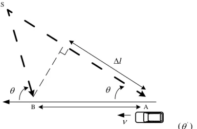
The relative motion between transmitter and receiver, consider a mobile moving at a constant velocity v , along a path segment having length d between points A and B, while it receives signals from a remote source S, as illustrated in Figure 1-1.
A B S l (')
Figure 1-1 Illustration of Doppler effect
The approximate path length traveled by the wave is represented as l while the
vehicle travels from point A to B, it can be expressed as:
l dc o s v tc o s (1.1) where t is the time required for the vehicle to travel from A to B. Since the source is assumed to be very far away, in order to simplify the deriving of Doppler shift, we
assumed that at point A and ' at point B is the same. The approximate amount of
phase shift and frequency shift fd experienced by the receiver can be described
as follows: 2 l 2v tcos (1.2) 1 cos . 2 d v f t (1.3)
stands for the wave length transmitted from the remote transmitter. Note that the
frequency shift fdand the phase shift are varying during the travel from point A
1.2 Time-Variant Channel Effect
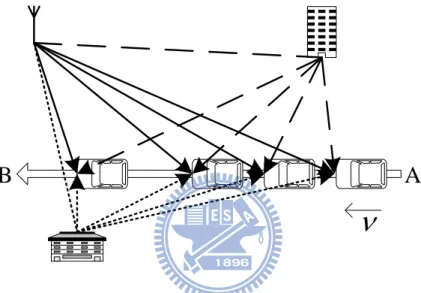
Multipath propagation with combination of Doppler shift induces time-variant channel effects. As the phenomenon shown in Figure 1-2, a vehicle receives three multipath components while it travels from point A to B. Each multipath component is affected by different time-varying frequency shift and phase shift, therefore the time-variant channel effect reveals.
B
A
Figure 1-2 The occasion of time-variant channels
The time-variant channel effect can also be described as a Finite Impulse Response (FIR) filter, which has three time-variant tap gains since there are three multipath components, as shown in Figure 1-3.
D D
w0(t) w1(t) w2(t)
s(t)
y(t)
Figure 1-3 A 3-tap Finite Impulse Response (FIR) filter model for time-variant channels
s t is the transmitted signal and the received signal y t
can be written as aconvolution sum
2
* kk=0
y t =
w t s t-k (1.4)Each time-variant tap gain wk
t is a complex number, which describes the phase andamplitude response of the kth path at time
t.
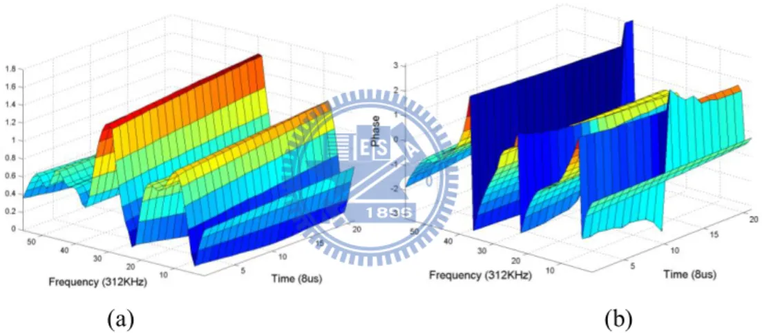
The time-variant tap gains, or Channel Impulse Response (CIR), can be transformed into Channel Frequency Response (CFR), which is also time-variant. Figure 1-4 shows the 15-tap noise-free time-variant CFR at 120km/hr by Jakes’ model [2].
(a) (b)
Figure 1-4 (a) Amplitude and (b) Phase variations of time-variant CFR by Jakes’ model at 120km/hr
Chapter 2
System Platform
3rd Generation Partnership Project (3GPP)[3][4][5] has recently specified an Orthogonal Frequency Division Multiplexing (OFDM) based technology, Evolved Universal Terrestrial Radio Access (E-UTRA), for support of wireless broadband data service up to 300 Mbps in the downlink and 75Mbps in the uplink [6]. In Long Term Evolution (LTE), MIMO technologies have been widely used to improve downlink peak rate, cell coverage, as well as average cell throughput. LTE is not only able to operate in different frequency bands but can also flexibly support different bandwidths.
A unique LTE possibility is to use different UL and DL bandwidths, allowing for asymmetric spectrum utilization. This is possible due to the support of both paired Frequency Division Duplexing (FDD) and unpaired Time Division Duplexing (TDD) band operations. In this thesis we concentrate on TDD.
2.1 LTE PHY Specification
Orthogonal Frequency Division Multiplexing (OFDM) is a popular method for high data rate wireless transmission. OFDM may be combined with antenna arrays at the transmitter and receiver to increase the diversity gain and to enhance the system capacity on time variant and frequency-selective channels, resulting in a multiple-input multiple-output (MIMO) configuration.
2.1.1 Transmitter
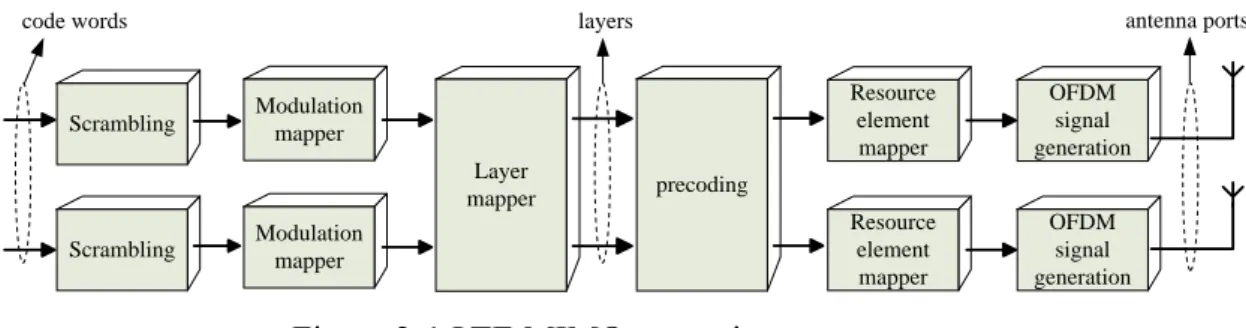
The transmitter block diagram of LTE MIMO specified is shown as Figure 2-1.
code words layers antenna ports
Scrambling Scrambling Modulation mapper Modulation mapper Resource element mapper Resource element mapper OFDM signal generation OFDM signal generation Layer mapper precoding
Figure 2-1 LTE MIMO transmitter
The baseband signal representing a downlink physical channel is defined in terms of the following steps:
- Scrambling of coded bits in each of the code words to be transmitted on a physical channel to prevent a succession of zeros or ones
- Modulation of scrambled bits from some modulation alphabet, e.g. BPSK, QPSK, 16QAM, 64QAM, to generate complex-values modulation symbols. - Mapping of complex-valued modulation symbols onto one or several
transmission layers. Basically a layer corresponds to a spatial multiplexing channel.
- The pre-coder extracts exactly one modulation symbol from each layer, jointly process these symbols, and maps the result in the frequency domain and antenna domain. The space-frequency block code (SFBC) as shown in section 2.2 is used if there has more than one transmit antennas.
- Mapping of complex-valued modulation symbols for each antenna port to the resource elements of the set of resource blocks assigned by the MAC scheduler for transmission of transport block(s).
signals appended to the Cyclic Prefix (CP) of 144 or 160 sub-carries are transmitted by RF modules.
2.1.2 Receiver
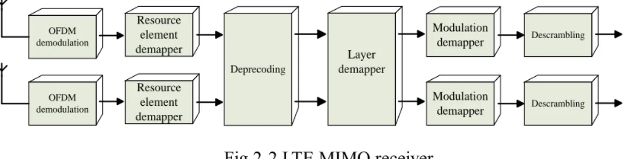
The receiver block diagram of MIMO-OFDM specified in LTE proposal is shown as Figure 2-2. OFDM demodulation OFDM demodulation Resource element demapper Resource element demapper Modulation demapper Modulation demapper Descrambling Descrambling Deprecoding Layer demapper
Fig 2-2 LTE MIMO receiver
The receive signals are first synchronized to recognize each OFDM symbol. Each OFDM symbols shall be processed and de-mapped to coded bits through the following steps:
- Each OFDM symbols is transformed to complex-valued frequency-domain OFDM signal by Fast Fourier Transform (FFT). If the OFDM symbol belongs to reference signal (described in section 2.1.4), then it is used for channel estimation.
- De-mapping complex-valued frequency-domain OFDM signal of each antenna port to complex-valued symbols.
- Complex-valued symbols are decoded by SFBC decoder, which needs the CFR information estimated by the channel estimation block. The SFBC decoder can be seen as the equalizer of MIMO-OFDM systems and it is introduced in section 2.2.
- After SFBC decoder, the spatial streams shall be Layer de-mapped and demodulation to complex-values modulation symbols.
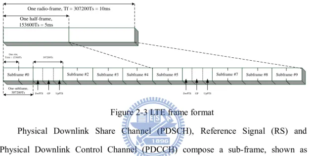
2.1.3 Frame Structure
Shown as Figure 2-3, frame structure is applicable to TDD. Each radio frame of
length Tf 307200 Ts 10ms consists of two half-frames of length
153600 Ts 5ms each. Each half-frame consists of five sub-frames of length
307200 Ts 1ms. One half-frame, 153600Ts = 5ms One radio-frame, Tf = 307200Ts = 10ms One slot, Tslot = 15360Ts 307200Ts One subframe, 307200Ts
Subframe #0 Subframe #2 Subframe #3 Subframe #4 Subframe #5 Subframe #7 Subframe #8 Subframe #9
DwPTS GP UpPTS DwPTS GP UpPTS
Figure 2-3 LTE frame format
Physical Downlink Share Channel (PDSCH), Reference Signal (RS) and Physical Downlink Control Channel (PDCCH) compose a sub-frame, shown as Figure 2-4. PDSCH is used for all user data, as well as for broadcast system information. Data is transmitted on the PDSCH in units known as transport blocks. A PDCCH carries a message known as Downlink Control Information (DCI), which includes resource assignments and other control information for a mobile or group of mobiles. RS(s) are known signals which do not carry any data. It can be used to do channel estimation. / / 7 OFDM symbols 1 OFDM symbol 1 OFDM symbol 2 OFDM symbols 2 OFDM symbols 1 OFDM symbol
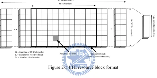
The transmitted signal in each slot is described by a resource grid of L M
subcarrier and N OFDM symbols, where L is downlink bandwidth configuration,
M is resource block size in the frequency domain, expressed as a number of
subcarriers, and N is the number of OFDM symbols in a downlink slot. Resource blocks are used to describe the mapping of certain physical channels to resource
elements. The resource grid structure is illustrated in Figure 2-5. In the thesis, Lis 50
blocks, Mrepresents 12 subcarriers, and N denotes 14 OFDM symbols.
O n e d o w n lin k s lo t T slo t N O F D M s y m b o ls Resource block (N*M resource elements) M subcarriers Resource element L*M subcarriers
N = Number of OFDM symbol L = Number of resource block M = Number of subcarrier
Figure 2-5 LTE resource block format
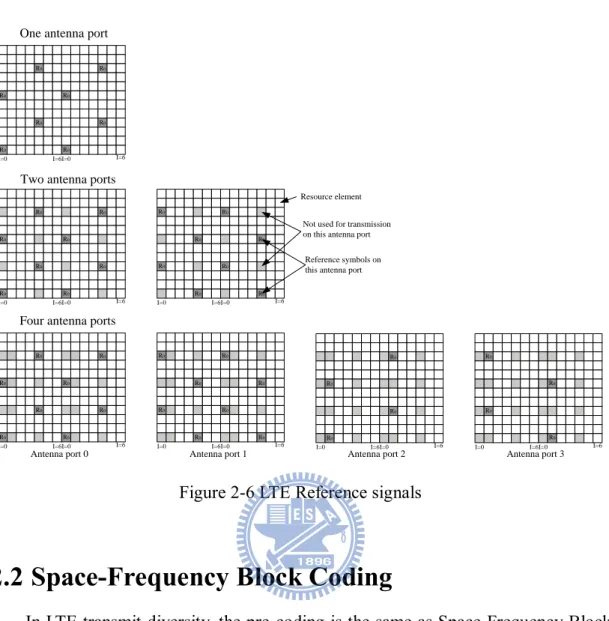
2.1.4 Reference Signal
LTE downlink reference signals have three types, Cell-specific reference signals, MBSFN reference signals, and UE-specific reference signals. In this thesis we concentrate on Cell-specific reference signals.
The mapping of downlink reference signals is shown in Figure 2-6. Resource element used for reference signal transmission on any of the antenna ports in a slot shall not be used for any transmission on any other antenna port in the same slot and set to zero.
One antenna port R0 R0 R0 R0 R0 R0 R0 R0
I=0 I=6I=0 I=6
R0 R0 R0 R0 R0 R0 R0 R0
I=0 I=6I=0 I=6
R0 R0 R0 R0 R0 R0 R0 R0
I=0 I=6I=0 I=6
Two antenna ports
Resource element
Not used for transmission on this antenna port
Reference symbols on this antenna port
R0 R0 R0 R0 R0 R0 R0 R0
I=0 I=6I=0 I=6
R0 R0 R0 R0 R0 R0 R0 R0
I=0 I=6I=0 I=6
Four antenna ports
R0
R0 R0
R0
I=0 I=6I=0 I=6
R0
R0 R0
R0
I=0 I=6I=0 I=6
Antenna port 0 Antenna port 1 Antenna port 2 Antenna port 3
Figure 2-6 LTE Reference signals
2.2 Space-Frequency Block Coding
In LTE transmit diversity, the pre-coding is the same as Space-Frequency Block Coding (SFBC) [7], it has been applied to frequency selective channels by using OFDM with cyclic prefix, which transforms a frequency selective channel into flat fading sub-channels. The SFBC coding is done across the sub-carriers inside one
OFDM symbol. In 22 SFBC, SFBC encodes two components onto two antennas
over two different frequencies, these two frequencies are chosen to correspond to adjacent subcarriers. Since channel realizations on adjacent subcarriers may differ, SFBC is more sensitive to large delay spreads.
2.2.1 2
2 SFBC
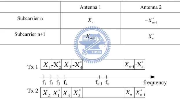
The block diagram on a transmitter using OFDM and space-frequency block coding is shown in Figure 2-7. The mapping scheme of the data symbols Xn for SFBCs with 2 transmit antennas is shown in Table 2-1. The mapping scheme for SFBCs is chosen such that on the first antenna the original data is transmitted without any modification so that the scheme is compatible to systems without SFBC where the second antenna is not implemented or switched off.
Table 2-1 Mapping with space-frequency block code and two transmit antenna
Antenna 1 Antenna 2 Subcarrier n n X * 1 n X Subcarrier n+1 1 n X Xn*
Tx 1
Tx 2
frequency
f
1f
2f
3f
4f
n-1f
n 1X
-X
*2X
3-X
*4X
n1-X
*n 2X
* 1X
X
3* * 1 nX
nX
4X
Figure 2-7 Space-frequency block coding in an OFDM transmitter
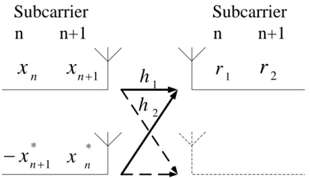
Two subcarriers x1 and x2 are about to be transmitted in two subcarriers periods
from two transmit antennas. The SFBC-encoded codeword is shown as Figure 2- 2-8. At frequency f1, x1 and
* 2
-x are transmitted through channels h1
andh2. And at frequency f2, x2 and * 1
x are transmitted through channels h1 andh2, respectively.
Subcarrier
n n+1
Subcarrier
n n+1
1 nx
nx
* nx
* 1 nx
1h
2h
1r
r
2Figure 2-8 22 SFBC MIMO systems for two receivers
Therefore the received signals r1 and r2 at time f1 and f2 can be expressed as
1 1 1 2 2 * 2 1 2 2 1 r =h x -h x r =h x +h x (2.1)
Rewrite in matrix form
1 1 2 1 * * * 2 2 1 2 r h -h x = , or R=H X r h h x (2.2)
The channel matrix H can be estimated using reference signals, hence the transmitted
symbols can be calculated by
-1 1 1 2 1 -1 * * * 2 2 1 2 x h -h r = , or X=H R x h h r (2.3)
Note that the dash-lined components, the second receiver and the two corresponded channels, are ignored during the derivation of the decoding process, since the decoding method is the same as the first receiver. In simulation platform, two receivers are deployed and the SFBC-decoded symbols for each receiver are averaged
2.3 Channel Models
In this section, the time-variant channel models are introduced, this channel model [2] is the well-known Jakes’ mode. It will describe as following.
2.3.1 Jakes’ Model
Time-variant channel effect can be modeled as a FIR filter with time-variant tap gains. For Jakes’ model, the variance of each tap gain obeys Rayleigh distribution. Figure 2-9 shows an n-tap FIR filter with Rayleigh-distributed tap gains, and the corresponded velocity is 120km/hr, shown for50ms .
Figure 2-9 FIR filter with Rayleigh-distributed tap gains at 120km/hr
D D w0(t) w1(t) wn-1(t)
...
...
s t
y t 50 ms - 10dB 0dB -10dB -30dB 0 Pha se A m pl itud e
s t is the transmitted signal and the received signal y t
can be written as a convolution sum
n-1
*k k=0
y t =
w t s t-k (2.4)The Rayleigh-distributed tap gains wk
t can be expressed as the sum ofsinusoids [8], that is
o o k c c s c N c n n m n=1 N s n n m n=1 w t =X (t)cos2 f t + X (t)sin2 f tX t =2 cos cos 2 f t + 2 cos cos 2 f t
X t =2 sin cos 2 f t + 2 sin cos 2 f t
(2.5) cf is the carrier frequency, and it equals to 2.4GHz in 802.11n. fm is the maximum
Doppler frequency shift described in equation (1.1) for =0 . No is the number of
oscillators that generate the sinusoid waveforms of angular frequencyn. Detail
Chapter 3
The Proposed Algorithm
In this chapter, an adaptive channel estimation technique is proposed. 22
SFBC for MIMO-OFDM systems is considered. The proposed algorithm consists of three parts, the channel estimation of initial channel, the decision-feedback adaptive channel estimation for estimating the noisy time-variant channel, and the frequency domain lose-pass filter for decreasing the SNR requirement.
Section 3.1 gives an overview of proposed decision-feedback adaptive channel estimation and the use PDCCH for channel estimation and frequency domain adaptive
channel estimation is proposed in section 3.2 and 3.3, the22SFBC is proposed in
3.4, and the lose-pass filter is discussed in section 3.5.
3.1 Adaptive Channel Estimation Overview
The synchronized time-domain signals are transformed into frequency-domain
OFDM symbols by FFT. Figure 3-1 describes the data path after FFT for 22 LTE
FFT Resource Element de-mapping Channel Estimation SFBC Decoder Adaptive channel Estimation Decision unit Low pass filter (PDCCH) M U X 1 r 2 r 1 h h2 1 X 2 X ' 1 (X)Decision ' 2 (X )Decision ' 2 X ' 1 X h1 2 h ' 1 h ' 2 h ' 2 ( )h filtered ' 1 ( )h filtered
Figure 3-1 22 adaptive channel estimation block diagram
After FFT, OFDM symbols classified as Physical Downlink Control Channel
(PDCCH) are used for channel estimation. The 22 SFBC decoder operates for every
two payload symbols, as shown as r1 and r2 above. Then the decoded symbols,
' 1
x
and '
2
x , are decided by decision unit. The functionality of the decision unit is illustrated in Figure 3-1, it uses QAM constellation for decisioning.
Decision Unit
Decoded symbol Decided symbol
' Decision X ' X XThe decided symbols are averaged with which of the second receiver. x1 and
2
x
are the differences between decided symbols and decoded symbols, and they are
used by adaptive channel estimation to obtain the variances of the time-variant
channels. After adding up with h1andh2, the time-variant channels,
' 1
h andh'2, are ready to update the channel information stored in channel estimation block. The usage of Low pass filter is to mitigate the influence of Additive White Gaussian Noise (AWGN), since the adaptive channel estimation algorithm is sensitive to noise.
The flow chart for adaptive channel estimation is show below.
PDCCH Channel N=1 N+1th OFDM Symbol has pilot? Use pilot to interpolation Nth OFDM Symbol channel ∆H N+1th OFDM Symbol Channel Channel Equalizer Adaptive Channel Estimation Step-size yes No N=N+1
Figure 3-3 Adaptive channel estimation flow chart
After use PDCCH to do initial channel estimation, the OFDM symbols can only be one of the following categories: reference signal (RS) for channel estimation, or
adaptive channel estimation. If the N1th OFDM symbol has RS, use these RS to
do interpolation, otherwise, use Nth OFDM symbol channel to do adaptive channel
3.2 Use PDCCH for Channel Estimation
Before adaptive channel estimation, it is necessary to estimation an OFDM symbol channel as initial channel. In this thesis, the PDCCH is used. Physical Downlink Control Channel (PDCCH) carries scheduling assignments and other control information. A physical control channel is transmitted on an aggregation of one of or several consecutive control channel elements (CCEs), where a control channel element corresponds to 9 resource element groups. The number of
resource-element groups not assigned to PCFICH or PHICH isNREG. The CCEs
available in the system are numbered from 0 andNCCE1, whereNCCE NREG/9. The
PDCCH supports multiple formats as listed in Table 3-1. Table 3-1: Supported PDCCH formats PDCCH format Number of CCEs Number of resource-element groups Number of PDCCH bits 0 1 9 72 1 2 18 144 2 4 36 288 3 8 72 576
As above describe, PDCCH are known signals which do not carry any data. In transmitted resource block, shows in Figure3-4. The PDCCH are second OFDM symbol and third OFDM symbol. We use the third OFDM symbol and zero forcing to
R0 R0 R0 R0 R0 R0 R0 R0
I=0 I=6 I=0 I=6
PDCCH
PDSCH
Third PDCCH OFDM symbol
Figure 3-4 PDCCH in resource block3.3 Frequency Domain Adaptive Channel Estimation
Each noisy time-variant channel estimated by adaptive channel estimation is then filtered by Low pass filter. For 2x2 LTE MIMO-OFDM systems, In an OFDM symbol, have 600 subcarriers. After SFBC decoder, there are 300 subcarriers. We get the 50 subcarriers, show in Figure 3-5, as virtual pilot to be adaptive channel estimation, pass through the SFBC coder and interpolation to 600 subcarriers, and then filtered by Low pass filter.OFDM symbol (600 subcarriers) Virtual pilot (50 subcarriers)
3.4 Adaptive Channel Estimation for 2
2 SFBC
In this section, the adaptive channel estimation algorithm can be seen as a transformation of the variances of SFBC-decoded symbols into the variances of time-variant channels. When we finish the one-shot channel estimation, if without adaptive channel estimation, we should keep a large memory to store the channel information until the step of channel equalizer. In architecture level, it will result huge number of gate count. The adaptive channel estimation algorithm applies to each frequency component individually for MIMO-OFDM systems.
For each receiver, the received signal within one SFBC block contains two subcarriers, r1andr2, which can be expressed as
1 1 1 2 2 2 1 2 2 1 ( ) r h x h x r h x h x (3.1) f
r indicates the received signal at frequency index f within SFBC block and the
channel from transmitter j is calledhj, which are assumed to be known. x1andx2
stands for the transmitted 2 2 SFBC codeword which are wanted.
By defining 1 * 2 r R r , 1 2 * * 2 1 h -h H h h and 1 2 x X x
, the received SFBC block
can be expressed in matrix form, that is
1 1 2 1 * * * 2 2 1 2 r h -h x = , or R=H X r h h x (3.2)
Due to time-variant channel effect, the channels of the consecutive SFBC block are not consistent with the previous ones. For the consecutive SFBC block, the channels
are assumed to be '
1
h andh'2, which are defined as
' 1 1 1 ' 2 2 2 h =h + h h =h + h (3.4) 1
h and h2 indicate the channel variance during one SFBC block duration.
Therefore, the received consecutive SFBC block in matrix form becomes
' ' 1 1 2 1 1 1 2 2 1 * * * '* '* * * * * 2 2 2 2 1 2 2 1 1 1 2 1 1 2 1 * * * * * * 2 2 2 1 2 1 1 2 2 r h -h x h + h -h - h x = = x x r h h h + h h h h -h x h - h x = + , x x h h h h or R=H X+ H X h - h where H h * * 1 h (3.5)
Applying the decoding process again, that is, multiplying the inverted channel
matrix -1
H on both left side of equation (3.5), hence
-1 -1 ' 1 1 ' DF DF 2 DF 2 H R=X+H H X X x x where X X + X= + x x (3.6)As shown above, in consequence of the time-variant channel effect, the decoded
symbol '
X contains a residual part with compared toX. The residual part X
indicates the variance of the decoded symbol due to time-variant channel effect. X
can be obtained if the time-variant channel effect is not strong enough to make for a
decision error on the decoded symbol '
X. That is, if the decision feedback result ofX',
which is defined asXDF, is equal to the ideal decoded symbolX, then the relationship
DF -1 DF DF DF -1 DF DF ' DF if X=X X +H H X =X + X H H X = X H X =H X where X=X -X (3.7)
H can be solved since it is the only unknown matrix in equation (3.7). Further
more, by defining 1 2 r R =H X r and 1 conj * 2 r R - r , equation (3.7) can be rewritten as
DF 1 2 1 1 DF * * 2 2 2 1 DF 1 DF 2 DF 1 1 * * * 2 2 1 2 DF DF -1 1 DF 2 DF 1 1 * * * 2 2 DF 1 DF 2 R=H X= H X h - h x r = x r h h x -x r h = h x x - r x -x r h = h x x - r (3.8)Since h1 and h2 are solved, ' 1
h and h'2 can be obtained by equation (3.4). Note that equation (3.8) uses the same process as which used in equation (3.3) for SFBC decoding.
3.5 First Order Low Pass Filter
Low pass filter is used on frequency domain to decrease the SNR requirements that adaptive channel estimation needed since it is sensitive to noise. The functionality of frequency domain Low pass filtering is illustrated below
a and b are vectors of low pass filter. It is show as Figure 3-6. Z-1 Z-1 Z-1
( )
x m
( ) b n b(3) b(2) b(1) ( ) y m ( ) a n a(3) a(2) 1( ) n Z m Z2( )m Z m1( )Chapter 4
Simulation Results
To evaluate the proposed algorithm, a typical MIMO-OFDM system based on
LTE is used as the reference design platform. Performance of the proposed 2 2
adaptive channel estimation under time-variant frequency-selective fast-fading channels is simulated. The parameters used in the simulation platform are: OFDM symbol length is 14 and 600 subcarriers in an OFDM symbol. The major parameters are summarized in Table 4-1.
Table 4-1 Simulation parameters
Parameter Value Number of taps 6 Doppler speed 120km/s Modulation 64-QAM Equalization Zero-Forcing FFT size 1024 Bytes Signal Bandwidth 20 MHz Subframe size 1ms
The results show that the best step-size in simulation is 0.1. Figure 4-2 expresses the Bit Error Rate (BER) performance with different step-size of the proposed adaptive
channel estimation for 22 LTE MIMO-OFDM systems under time-variant channels
for 120km/hr Jakes’ model.
Figure 4-1 MSE of OFDM symbol with step-size 0, 0.1, 0.15, 0.2
Figure 4-3 addresses the Bit Error Rate (BER) performance of the proposed
adaptive channel estimation 22 LTE MIMO-OFDM systems, which use the low pass
filter to filter the noisy.
Figure 4-3 BER of OFDM symbol with Low pass filter
Figure 4-4 indicates the Bit Error Rate (BER) performance of the proposed
adaptive channel estimation 22 LTE MIMO-OFDM systems, which use the different
initial channel estimation. The first one is use first OFDM symbol’s reference signal, and be interpolation as initial channel, the other one use the PDCCH to estimate the initial channel. The results show that use PDCCH to estimate the initial channel has the better performance.
Figure 4-4 BER of OFDM symbol with two channel estimation methods. The required SNR for BER of the proposed algorithm among various configurations are summarized in Table 4-3.
Table 4-3 Required SNR for BER (64-QAM modulation)
Simulation configurations Jakes’ model 120km/hr with step-size 0.1 Jakes’ model 120km/hr with step-size 0.15 Jakes’ model 120km/hr with step-size 0.2 2 2 MI MO -O F D M s y st e m
s One-shot channel estimation
One-tap compensation
27 dB 27 dB 27 dB
Adaptive channel estimation Direct compensation
38 dB 40 dB 45 dB
Adaptive channel estimation low pass filter compensation
As introduction described, the contribution of proposed adaptive channel estimation is computing complexity reduced which compared with one-shot channel estimation. Table 4-2 exhibits the comparison between the one-shot channel and proposed adaptive channel estimation. The result shows that the one-shot channel estimation needs 600×14 storages to store the channel information, but proposed adaptive channel estimation only needs 600 storages. In channel estimation, the multiplier number of one-shot channel estimation needs 650000, but the proposed algorithm which use PDCCH only needs 900, and in adaptive channel estimation, one-shot channel estimation needs zero multiplier and proposed algorithm needs 75000 multipliers. For estimate channel, the total multiplier number of one-shot channel estimation is 650000, and proposed algorithm is 75900. The computing complexity of proposed algorithm is reduced.
Table 4-2 complexity comparison between two channel estimation
Channel Estimation One-shot Adaptive (use first OFDM
symbol) Adaptive (use PDCCH) Storages 600 × 14 600 600 Multiplier (channel Estimation) 650000 1800 900 Multiplier (Adaptive channel Estimation) 0 75000 75000
Chapter 5
Conclusion and Future Work
5.1 Conclusion
In this thesis, adaptive channel estimation is proposed to oppose the Doppler effect under high velocity environments, and make full use of the time- and frequency-domain correlation of the frequency response of time-varying multipath fading channels without requirement of accurate channel statistics.
The presented 22 adaptive channel estimation scheme achieves. It is a
prototype algorithm for SFBC-coded MIMO-OFDM systems. The distance between QAM constellation points dominates the maximum tolerance to time-variant channels; therefore lower modulation scheme provides higher velocity tolerance. Further more, the proposed adaptive channel estimation algorithm shares the same process with SFBC decoding. It is a significant feature in hardware implementation phase.
5.2 Future Work
High QAM constellation like 256-QAM for higher data rate is going to be deployed. As a result, the distance between constellation points shrinks; therefore a robust decision scheme is demanded. Since QAM decisioning simply outputs the closest constellation points to the input as its decision, FEC-feedback decisioning can be considered.
Bibliography
[1] Theodore S. Rappaport, “Wireless Communications – Principles and Practice,
2nd edition”, chapter 5, Prentice-Hall, 2002
[2] P. Dent, G. Bottomley and T. Croft, “Jakes Fading Model Revisited”, IEE Electronics Letters, p.1162~p.1163, June 1993
[3] 3GPP, “Evolved universal terrestrial radio access (E-UTRA); long term evolution (LTE) physical layer; general description,” 36.201,V8.3.0.
[4] “Evolved universal terrestrial radio access (E-UTRA) and evolved universal terrestrial radio access network (E-UTRAN); overall descrip- tion; stage 2,” 36.300,V9.0.0.
[5] 3GPP, TS 36.211, “Evolved Universal Terrestrial Radio Access(E-UTRA); LTE Physical Channel and Modulation (Release8)”
[6] 3GPP, TS 36.201, “Evolved Universal Terrestrial Radio Access(E-UTRA); LTE Physical Layer-General Description (Release8)”.
[7] S. M. Alamouti, “A Simple Transmitter Diversity Scheme for Wireless Communications,” IEEE J. Select. Areas Communication, vol. 16, no. 8, pp. 1451-1458, 1998.
[8] W. C. Jakes, Ed., “Microwave Mobile Communications”, IEEE Press, Piscataway, NJ, 1974
[9] Ming-Yeh Wu, “Design of Pilot-based Adaptive Equalization for Wireless
OFDM Baseband Applications”, NCTU thesis, 2004
[10] Jos Akhtman and Lajos Hanzo, “Advanced Channel Estimation for , IEEE Transactions, Mar. 2007
[13] Chia-Chun Hung, “On the Detection of Coded MIMO-OFDM Signals in
Time-Varying Channels”, NCTU thesis, 2005
[14] Chin-Jung Tsai, “Design of Channel Estimation and Data Detection for OFDM