粒子群演算法於多目標排程問題之研究

國 立 交 通 大 學

工 業 工 程 與 管 理 學 系

博士論文

粒子群演算法於多目標排程問題之研究

A Study of Particle Swarm Optimization for

Multi-objective Production Scheduling Problems

研究生 ： 林信宏

指導教授 ： 沙永傑 教授

洪瑞雲 教授

粒子群演算法於多目標排程問題之研究

A Study on Particle Swarm Optimization for Multi-objective

Production Scheduling Problems

研 究 生： 林信宏

Student： Hsing-Hung Lin

指導教授： 沙永傑

Advisor： Dr. D. Y. Sha

洪瑞雲

Dr. R. Y. Horng

國 立 交 通 大 學

工 業 工 程 與 管 理 學 系

博 士 論 文

A Dissertation

Submitted to Department of Industrial Engineering and Management

College of Management

National Chiao Tung University

in Partial Fulfillment of the Requirements

for the Degree of

Doctor of Philosophy

in

Industrial Engineering and Managemen

June 2010

Hsinchu, Taiwan, Republic of China

I

粒子群演算法於多目標排程問題之研究

研究生：林信宏 指導教授： 沙永傑博士 洪瑞雲博士 國立交通大學工業工程與管理系

摘

摘

摘

摘 要

要

要

要

以往學術上排程問題的研究主流是尋找單一目標的最佳解(如: 最小完工時 間) ，然而，實務上生產製造系統的排程需求是達成多目標最佳化。由於運算時 間與成本的考量，過去的許多研究已經發展出許多演算法則以搜尋最佳解或近似 最佳解。 在 本 篇 論 文 中 ， 我 們 分 別 提 出 適 合 求 解 流 程 型 排 程 問 題 (Flow Shop Scheduling Problem, FSSP)、零工型排程問題(Job Shop Scheduling Problem, JSSP)

與開放型排程問題(Open Shop Scheduling Problem, OSSP)的粒子群最佳化演算法 (Particle Swarm Optimization, PSO)。本研究所提出的演算法針對三種典型排程問

題，以同時達到最小完工時間(Makespan)、總流程時間(Total flow time)與機器閒 置時間(Machine idle time)作為目標。

粒子群演算法是一種群體搜尋最佳化演算法，於 1995 年被提出。原始的 PSO 是應用於求解連續最佳化問題。因為排程問題為一離散最佳化問題，我們必須修 改粒子位置、粒子移動以及粒子速度的表達方式，讓 PSO 更適於求解排程問題。

對於 FSSP 與 JSSP，本研究比較 PSO 與文獻中的基因演算法(Genetic Algorithm, GA)搜尋三大目標的結果，顯示本文提出的 PSO 優於基因演算法。本

研究另行發展求解多目標 OSSP 的基因演算法並與 PSO 進行 Benchmark 問題的 比較，計算結果顯示，修改後的 PSO 所搜尋到的解，在品質與效率上優於基因 演算法。

A Study on Particle Swarm Optimization for Multi-objective

Production Scheduling Problems

Student：Hsing-Hung Lin Advisor： Dr. D. Y. Sha

Dr. R. Y. Horng Department of Industrial Engineering and Management

National Chiao Tung University

ABSTRACT

The academic approach of discovering the single optimal solution (ex. makespan) of

scheduling for production system is the mainstream although the empirical

requirement of production system is to achieve multi-objective optimization. Many

algorithms have been developed to search for optimal or near-optimal solutions due to

the computational cost of determining exact solutions.

This study provides a Particle Swarm Optimization (PSO) to elaborate

multi-objective flow shop scheduling problem (FSSP), job shop scheduling problem

(JSSP) and open shop scheduling problem (OSSP). The proposed evolutionary

algorithm searches the optimal solution for objectives by considering the makespan,

total flow time, and machine idle time simultaneously.

Particle Swarm Optimization (PSO) is a population-based optimization algorithm,

which was developed in 1995. The original PSO is used to solve continuous

optimization problems. Due to the discrete solution spaces of scheduling optimization

problems, the authors modified the particle position representation, particle movement,

and particle velocity in this study. The modified PSO could be applied for solving

various benchmark problems; moreover, the results demonstrated that the modified

PSO outperformed traditional evolutionary heuristics – Genetic Algorithm in

searching quality and efficiency.

Keywords: Particle swarm optimization, Multi-objective, Flow shop scheduling, Job shop scheduling problem, Open shop scheduling

III

致

致

致

致 謝

謝

謝

謝

時光荏苒，一轉眼已經過了六年，終於我也可以寫下論文的致謝辭。在博士 求學過程間，首先要感謝的是指導教授沙永傑老師，除了在研究期間給我精神上 的支持外，也在出國參加研討會發表論文時，給予相當多的實質幫助。其次，必 須感謝的是共同指導教授洪瑞雲老師，協助處理校內相關的行政規定與作業，使 我得以順利取得學位。另外，感謝論文口試委員，系上老師彭德保教授、中華大 學謝玲芬教授、台灣科技大學王孔政教授、以及雲林科技大學駱景堯教授，在論 文計劃書及最後口試期間提供許多寶貴的建議，由於他們的意見，使本篇論文更 加豐富與完善。 感謝論文研究期間一直提供幫助的誠佑學長，還要感謝共同修課，一起打球 的同學們：新恩、家寧、國良、崑智、俊雄、彰孚、雅甄、惠誠、志偉、清章。 最後要感謝家人支持，父母親六年間不辭辛勞的協助照顧襁褓中的兒女，也 感謝儀鵑一路以來的陪伴，工作同時還要花費心思照料家庭，更付出許多心力叮 嚀剛開始學習成長的女兒，有了家人的協助，使我可以在無後顧之憂下，全力完 成學業。

CONTENTS

中文摘要 中文摘要 中文摘要 中文摘要 ... ⅠⅠⅠ Ⅰ ABSTRACT ... ⅡⅡⅡ Ⅱ 致謝 致謝 致謝 致謝 ….………. ⅢⅢⅢⅢ CONTENTS ... ⅣⅣⅣ Ⅳ LIST OF FIGURES ... ⅥⅥⅥ Ⅵ LIST OF TABLES ... ⅦⅦⅦ Ⅶ CHAPTER 1 INTRODUCTION ... 1 1.1 Research Motivations ... 1 1.2 Research Objectives ... 2 1.3 Research Process ... 2 1.4 Organization ... 3

CHAPTER 2 LITERATURE REVIEW ... 4

2.1 Particle Swarm Optimization ... 4

2.2 Genetic Algorithm ... 6

2.3 Flow Shop Scheduling Problem ... 7

2.4 Job Shop Scheduling Problem ... 10

2.5 Open Shop Scheduling Problem ... 13

2.6 Multiple Objective Programming... 15

CHAPTER 3 PSO FOR MULTI-OBJECTIVE FSSP ... 19

3.1 Problem Formulation ... 19

V

3.3 Particle Velocity ... 23

3.4 Particle Movement ... 24

3.5 Pareto optimal set maintenance ... 26

3.6 Computational Results ... 28

CHAPTER 4 PSO FOR MULTI-OBJECTIVE JSSP ... 48

4.1 Problem Formulation ... 48

4.2 Particle Position Representation... 48

4.3 Particle Velocity ... 51

4.4 Particle Movement ... 52

4.5 Diversification strategy ... 54

4.6 Computational Results ... 55

CHAPTER 5 PSO FOR MULTI-OBJECTIVE OSSP ... 74

5.1 Problem Formulation ... 74

5.2 Particle Position Representation... 74

5.3 Particle Velocity ... 76

5.4 Particle Movement ... 77

5.5 Computational Results ... 79

CHAPTER 6 CONCLUSIONS AND FUTURE STUDIES ... 96

6.1 Conclusions ... 96

6.2 Future Studies ... 98

Appendix ……….……….100

LIST OF FIGURES

FIGURE 1.1THE FLOW CHART OF THIS DISSERTATION _{... 3}

FIGURE 3.1THE CONVERSION BETWEEN INTEGERS AND FLOAT-POINT NUMBERS _{... 22}

FIGURE 3.2THE PRIORITY LIST STORED IN THE ARRAY ... 22

FIGURE 3.3THE PRIORITY LIST CHANGED AS PARTICLE MOVEMENT _{... 22}

FIGURE 3.4A NEW PERMUTATION LIST ... 23

FIGURE 4.1EXAMPLE OF _{JSSP ... 54}

FIGURE 4.2FINDING THE LOCATION TO EXCHANGE _{... 54}

FIGURE 4.3EXCHANGE OPERATION OF _{PSO ... 54}

FIGURE 4.4THE FACTOR RESPONSE DIAGRAM OF S/N RATIO DIAGRAM OF 15×15 PROBLEM _{... 57}

FIGURE 4.5THE FACTOR RESPONSE DIAGRAM OF S/N RATIO DIAGRAM OF 20×15 PROBLEM _{... 58}

FIGURE 4.6THE FACTOR RESPONSE DIAGRAM OF S/N RATIO DIAGRAM OF 20×20 PROBLEM _{... 59}

FIGURE 4.7THE FACTOR RESPONSE DIAGRAM OF S/N RATIO DIAGRAM OF 30×15 PROBLEM _{... 61}

FIGURE 4.8THE FACTOR RESPONSE DIAGRAM OF S/N RATIO DIAGRAM OF 30×20 PROBLEM _{... 62}

FIGURE 4.9THE FACTOR RESPONSE DIAGRAM OF S/N RATIO DIAGRAM OF 50×15 PROBLEM _{... 63}

FIGURE 4.10THE FACTOR RESPONSE DIAGRAM OF S/N RATIO DIAGRAM OF 50×20 PROBLEM _{... 65}

FIGURE 5.1THE SCATTER DIAGRAMS OF GP8 ... 94

FIGURE 5.2THE SCATTER DIAGRAMS OF GP9 ... 95

VII

LIST OF TABLES

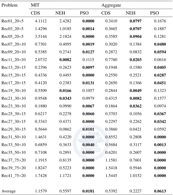
TABLE 3.1THE AVERAGE RELATIVE ERROR IN CMAX AND MFT OF PROBLEM RECXX .... 31

TABLE 3.2THE AVERAGE RELATIVE ERROR IN MIT AND AGGREGATE OF PROBLEM REC ... 32

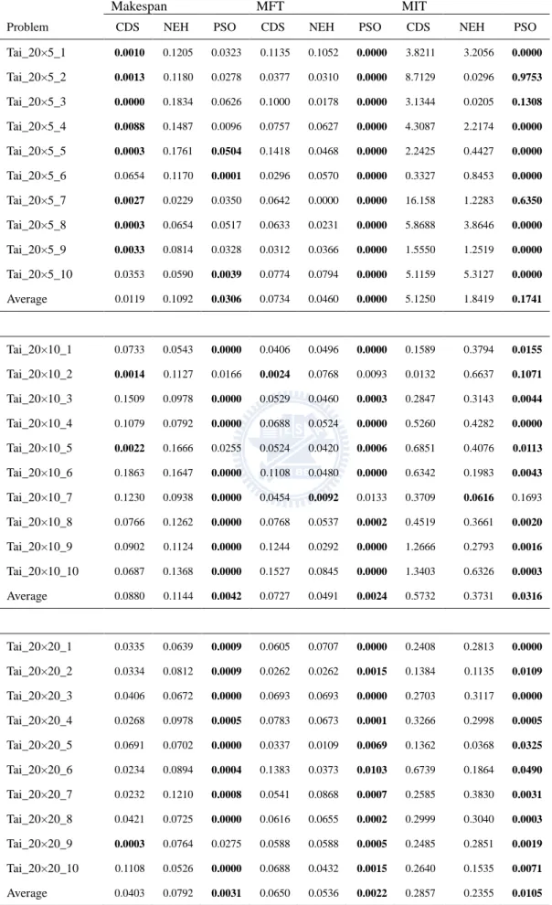
TABLE 3.3THE AVERAGE RELATIVE ERROR IN CMAX ,MFT AND MIT OF PROBLEM TAI_20 ... 33

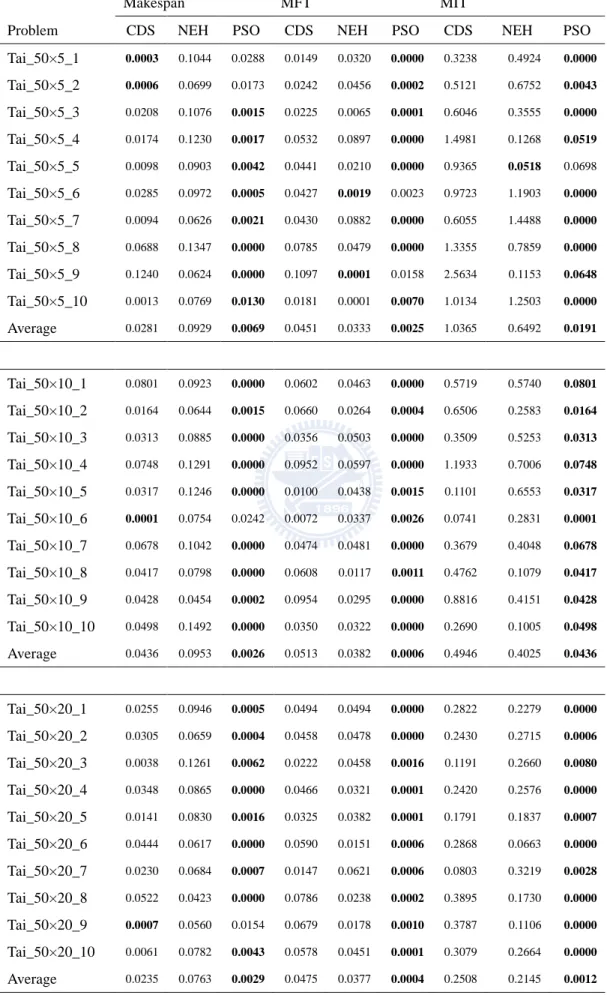
TABLE 3.4THE AVERAGE RELATIVE ERROR IN CMAX ,MFT AND MIT OF PROBLEM TAI_50 ... 34

TABLE 3.5THE AVERAGE RELATIVE ERROR IN CMAX ,MFT AND MIT OF PROBLEM TAI_{_100 ... 35}

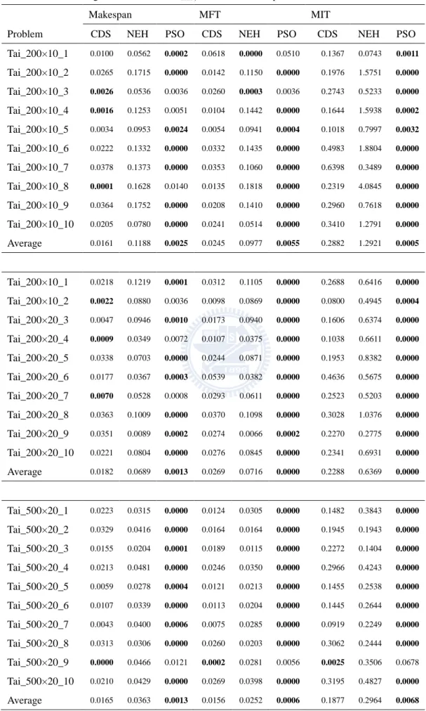
TABLE 3.6THE AVERAGE RELATIVE ERROR IN CMAX ,MFT AND MIT OF PROBLEM TAI_200 AND TAI_{_500 ... 36}

TABLE 3.7THE AGGREGATE PERFORMANCE OF PROBLEM TAI20×5 TO TAI_{50×20 ... 37}

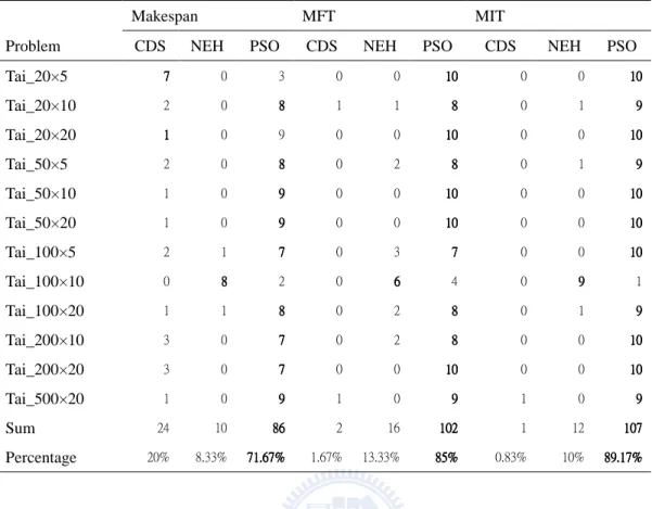
TABLE 3.8THE NUMBER AND PERCENTAGE OF PROBLEMS FOR DIFFERENT OBJECTIVE WITH SUPERIOR RESULTS _{... 39}

TABLE 3.9THE NUMBER OF PROBLEMS FOR AGGREGATE OBJECTIVES WITH SUPERIOR RESULTS _{... 39}

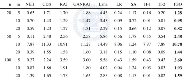
TABLE 3.10COMPARISON OF MAKESPAN(MS) FOR DIFFERENT HEURISTICS_{. ... 42}

TABLE 3.11COMPARISON OF TOTAL FLOW TIME (TFT) FOR DIFFERENT HEURISTICS _{... 42}

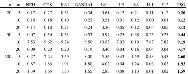
TABLE 3.12COMPARISON OF MACHINE IDLE TIME (MIT) FOR DIFFERENT HEURISTICS _{. 43} TABLE 3.13SUMMATION OF MS,TFT AND MIT FOR DIFFERENT HEURISTICS _{... 43}

TABLE 3.14AVERAGE CPU TIME (IN SECONDS_{) ... 44}

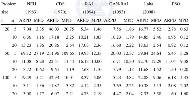
TABLE 3.15COMPARISON OF TOTAL FLOW TIME (TFT) FOR HEURISTICS IN _{ARPD ... 44}

TABLE 3.16COMPARISON OF TOTAL FLOW TIME (TFT) FOR HEURISTICS IN _{MPD ... 45}

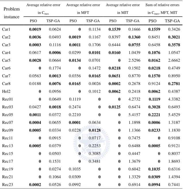
TABLE 3.17THE RESULTS OF _{TSP_GA ... 45}

TABLE 3.18THE AVERAGE RELATIVE ERROR OF PSO AND _{TSP-GA ... 47}

TABLE 4.1AN 2×2 EXAMPLE ... 50

TABLE 4.2THE PARAMETER OF PSO ... 56

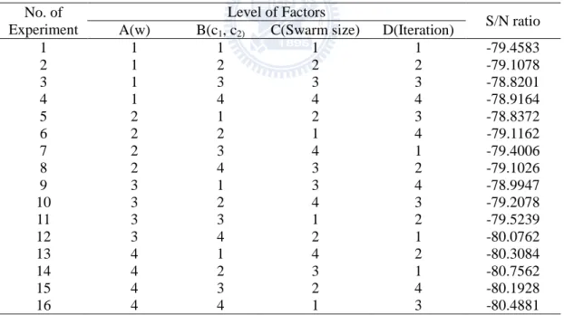
TABLE 4.3THE L16 ORTHOGONAL ARRAY AND S/N RATION OF 15×15 PROBLEM ... 56

TABLE 4.4THE FACTORS RESPONSE OF 15×15 PROBLEM ... 56

TABLE 4.5THE BEST LEVEL OF FACTORS OF 15×15 PROBLEM ... 57

TABLE 4.6THE L16 ORTHOGONAL ARRAY AND S/N RATION OF 20×15 PROBLEM ... 57

TABLE 4.7THE FACTORS RESPONSE OF 20×15 PROBLEM ... 58

TABLE 4.8THE BEST LEVEL OF FACTORS OF 20×15 PROBLEM ... 58

TABLE 4.9THE L16 ORTHOGONAL ARRAY AND S/N RATION OF 20×20 PROBLEM ... 59

TABLE 4.11THE BEST LEVEL OF FACTORS OF 20×20 PROBLEM _{... 59}

TABLE 4.12THE L16 ORTHOGONAL ARRAY AND S/N RATION OF 30×15 PROBLEM ... 60

TABLE 4.13THE FACTORS RESPONSE OF 30×15 PROBLEM _{... 60}

TABLE 4.14THE BEST LEVEL OF FACTORS OF 30×15 PROBLEM _{... 61}

TABLE 4.15THE L16 ORTHOGONAL ARRAY AND S/N RATION OF 30×20 PROBLEM ... 61

TABLE 4.16THE FACTORS RESPONSE OF 30×20 PROBLEM _{... 62}

TABLE 4.17THE BEST LEVEL OF FACTORS OF 30×20 PROBLEM _{... 62}

TABLE 4.18THE L16 ORTHOGONAL ARRAY AND S/N RATION OF 50×15 PROBLEM ... 63

TABLE 4.19THE FACTORS RESPONSE OF 50×15 PROBLEM _{... 63}

TABLE 4.20THE BEST LEVEL OF FACTORS OF 50×15 PROBLEM _{... 64}

TABLE 4.21THE L16 ORTHOGONAL ARRAY AND S/N RATION OF 50×20 PROBLEM ... 64

TABLE 4.22THE FACTORS RESPONSE OF 50×20 PROBLEM _{... 64}

TABLE 4.23THE BEST LEVEL OF FACTORS OF 50×20 PROBLEM _{... 65}

TABLE 4.24COMPARISON OF MOGA AND MOPSO FOR MAKESPAN _{... 67}

TABLE 4.25COMPARISON OF MOGA AND MOPSO FOR TOTAL IDLE TIME _{... 68}

TABLE 4.26COMPARISON OF MOGA AND MOPSO FOR TOTAL TARDINESS _{... 69}

TABLE 4.27COMPARISON OF MOGA AND MOPSO WITH THREE OBJECTIVES _{... 70}

TABLE 4.28THE RESULTS OF SOLVING FT,ABZ,ORB AND YN WITH _{MOPSO ... 71}

TABLE 4.29THE RESULTS OF SOLVING LA WITH _{MOPSO ... 72}

TABLE 4.30THE RESULTS OF SOLVING SWV WITH _{MOPSO... 73}

TABLE 5.1THE RESULTS OF THE FIRST EXPERIMENT CONSIDERING THREE OBJECTIVES AS PARETO SET ... 80

TABLE 5.2THE RESULTS OF THE FIRST EXPERIMENT CONSIDERING MAKESPAN AND TOTAL FLOW TIME AS PARETO SET ... 80

TABLE 5.3THE RESULTS OF THE FIRST EXPERIMENT CONSIDERING MAKESPAN AND MACHINE IDLE TIME AS PARETO SET ... 81

TABLE 5.4THE RESULTS OF THE FIRST EXPERIMENT CONSIDERING TOTAL FLOW TIME AND MACHINE IDLE TIME AS PARETO SET ... 81

TABLE 5.5SUMMARY OF THE RESULTS OF THE FIRST EXPERIMENT ... 82

TABLE 5.6THE RESULTS OF THE SECOND EXPERIMENT CONSIDERING THREE OBJECTIVES WITH THREE SUB-SWARMS ... 82

TABLE 5.7THE RESULTS OF THE SECOND EXPERIMENT CONSIDERING MAKESPAN WITH ONE SWARM ... 83

TABLE 5.8THE RESULTS OF THE SECOND EXPERIMENT CONSIDERING TOTAL FLOW TIME WITH ONE SWARM ... 83

TABLE 5.9THE RESULTS OF THE SECOND EXPERIMENT CONSIDERING MACHINE IDLE TIME WITH ONE SWARM ... 84

IX

TABLE 5.10THE RESULTS OF THE SECOND EXPERIMENT CONSIDERING MAKESPAN AND

TFT WITH TWO SUB-SWARMS _{... 84}

TABLE 5.11THE RESULTS OF THE SECOND EXPERIMENT CONSIDERING MAKESPAN AND MIT WITH TWO SUB-SWARMS _{... 85}

TABLE 5.12THE RESULTS OF THE SECOND EXPERIMENT CONSIDERING TFT AND MIT WITH TWO SUB-SWARMS _{... 85}

TABLE 5.13SUMMARY OF THE RESULTS OF THE SECOND EXPERIMENT _{... 86}

TABLE 5.14THE RESULTS OF MOPSO FOR BENCHMARK PROBLEMS GP03-GP_{10 ... 87}

TABLE 5.15THE RESULTS OF MOGA FOR BENCHMARK PROBLEMS GP03-GP_{10 ... 90}

TABLE 5.16THE COMPARISON OF MOPSO AND MOGA FOR MAKESPAN _{... 93}

TABLE 5.17THE COMPARISON OF MOPSO AND MOGA FOR MACHINE IDLE TIME _{... 93}

CHAPTER 1

INTRODUCTION

1.1 Research Motivations

Scheduling is an optimization process by which limited resources are allocated over

time among parallel and sequential activities. Such situations develop routinely in

factories, publishing houses, shipping universities, hospitals, airports, etc. Solving

such a problem amounts to making discrete choice such that an optimal solution is

found among a finite or a countable infinite number of alternatives. Such problems are

called combinational optimization problems. Typically, the task is complex, limiting

the practical utility of combinatorial, mathematical programming and other analytical

methods in solving scheduling problems effectively.

To find exact solutions of scheduling problems a branch-and-bound or dynamic

programming algorithm is often used. However, many shop scheduling problems are

NP-hard, which means that the problem cannot be exactly solved in a reasonable

computation time. Using problem-specific information sometimes reduces search

space, even though the problem is still difficult to solve exactly. Therefore, heuristic

algorithms and dispatching rules are developed to obtain the approximate optimal

solution. Meta-heuristic is one of the most popular and the most efficient method to

obtain the approximate optimal solution. Among the meta-heuristics, particle swarm

optimization (PSO) is new and extensively implemented in recent years. However, the

original intent of PSO is to solve continuous optimization problems, and PSO

1.2 Research Objectives

The objective of this work is to development PSOs for two shop scheduling problems:

the flow shop scheduling problem (FSSP) and the job shop scheduling problem

(JSSP). In the work of FSSP, the problem is to find a schedule to minimize the

makespan (C_max), mean flow time and machine idle time. In the work of JSSP, we attempt to search a schedule to minimize the makespan (Cmax), machine idle time and

total tardiness.

Since the original intent of PSO is to solve continuous optimization problems,

we have to modify the original PSO when we implement PSO to a combinatorial

optimization problem. PSO can be separated several parts to discuss: position

representation, particle velocity, and particle movement. We will develop various PSO

designs in this work. On the other hand, the PSO developed in this work can be an

example of PSO design for other discrete optimization problems.

1.3 Research Process

The research of this dissertation begins with the determination of research topic. The

literature consists with flow shop scheduling, job shop scheduling, open shop

scheduling, particle swarm optimization and genetic algorithms. The programs of

particle swarm optimization and genetic algorithm are coded with programming

language C according to the types of scheduling problem. Then, the experiments are

compared to evaluate the performance of each algorithm to different problem types.

Figure 1. 1 The flow chart of this dissertation

1.4 Organization

The organization of the remaining chapters for this research is as follows. Chapter 2

reviews the literatures of the background of shop scheduling problems and PSO.

Chapter 3 describes the factors of PSO design and PSO for FSSP. PSO for JSP is

modified and illustrated in Chapter 4. We also proposed a novel PSO for OSSP in

Chapter 5. In chapter 6 we draw our conclusion and indicate the direction for further

research. Research Topic Literature Review PSO Algorithm Coding Experiment Comparison Conclusion

CHAPTER 2

LITERATURE REVIEW

2.1 Particle Swarm Optimization

Particle swarm optimization (PSO) is an evolutionary technique for unconstrained

continuous optimization problems proposed by Kennedy and Eberhart (1995). The

PSO concept is based on observations of the social behavior of animals such as birds

in flocks, fish in schools, and swarm theory. The advantages of the PSO method:

simple structure, immediate applicability to practical problems, ease of

implementation, quick solution, and robustness. Particle swarm optimization proposed

recently for unconstrained continuous optimization problems is one of the latest

evolutionary techniques. PSO has been successfully applied to different field of

applications due to the easy implementation and computational efficiency.

Nevertheless, the applications of the PSO on the combination optimization problem

are still scarce.

The major idea of PSO is based on observations of the social behaviors of

animals such as bird flocking, fish schooling, and swarm theory. The population is

initialized by random solutions. The population consists with individuals (i.e.

particles). Each particle is assigned with a randomized velocity according to its own

and populations’ movement experience. The relationship between swarm and particles

in PSO is similar to the relationship between population and chromosomes in GA.

In PSO, the problem solution space is formulated as a search space. Each

position of the particles in the search space is a correlated solution of the problem.

Particles cooperate to find out the best position (solution) in the search space (solution

Suppose that the searching space is D-dimensional and ρ particles comprise the

swarm. Each particle locates at the position say Xi={x1i, x2i, …, xDi} with the velocity

Vi={v1i, v2i, …, vDi}, where i=1, 2, …,ρ. Based on the PSO algorithm, each particle

move toward its own best position (pbest) denoted as Pbesti={pbest1i, pbest2i,…,

pbestni} and the best position of the whole swarm (gbest) denoted as Gbest={gbest1,

gbest2, …, gbestn}with each iteration. Each particle changes its position according to

its velocity which is randomly generated toward pbest and gbest positions. For each

particle r and dimension s, the new velocity vsr and position xsr of particles can be

calculated by the following equations:

) ( ) ( 2 2 1 1 kj kj j kj kj

kj w v c rand pbest x c rand gbest x

v ← × + × × − + × × − (2.1)

kj kj kj x v

x ← + (2.2)

In Eqs. (2.1) and (2.2), τ means the iteration number. The inertia weight w is

employed to control exploration and exploitation. A large w keeps particles with high

velocity and prevents particles from trapping in local optima. A small w maintains low

velocity of particles and urges particles to exploit the same search area. The constant

c1 and c2 are acceleration coefficients to determine whether particles prefer to move closer to pbest position or gbest position. The rand1 and rand2 are two independent

random numbers uniformly distributed between 0 and 1. The termination criterion of

the PSO algorithm includes the maximal number of generations, designated value of

pbest and no further improved pbest. The standard process of PSO is outlined as follows:

(1)Initialize a population of particles with random positions and velocities on d

dimensions in the search space.

(3)Update the position of each particle, according to Eq. (2.2).

(4)Map the position of each particle into solution space and evaluate its fitness

value according to the desired optimization fitness function. Meanwhile,

update pbest and gbest position if necessary.

(5)Loop to Step2 until a criterion is met, usually a sufficient good fitness or a

maximum number of iterations.

The original PSO is designed to suit continuous solution space. For better

applying to combinational optimization problems, we have to modify PSO position

representation, particle velocity, and particle movement.

2.2 Genetic Algorithm

The concept of genetic algorithms (GA) was introduced by Holland (1975) as a

general search technique which mimics biological evolution, with the survival of the

fittest individuals and a structured, yet randomized, information exchange like in

population genetics. GAs have been applied with a growing success to combinational

problems (Reeves, 1996). GAs works on a set (population) of solutions. Each solution

is encoded as a string of symbols called chromosome, and is associated with a

measure of adaptation, the fitness, often related to the objective function. Starting

from an initial population, new solutions are generated by selecting some parents

randomly, but with a probability growing with fitness, and by applying genetic

operators such as crossover (an exchange of substrings of the parent chromosomes)

and mutation (a random perturbation of a chromosome). Some existing solutions are

then selected at random and replaced by some of the offspring, to keep a constant

For solving optimization problems, genetic algorithms have been investigated

and shown to be effective at exploring a large and complex space in an adaptive way

guided by the equivalent biological evolution mechanism (Huang and Adeli, 1994).

Many conventional optimization methods start from one point in the search area and

then move sequentially to achieve the optimal solution, thereby operating rather

locally and highly prone to falling inside a coincidental local optimum.

GAs are known for their robustness: they can be applied to a wide range of

problems without special knowledge about the problem structure. The price to pay is

that they cannot compete with meta-heuristics which explore problem-specific

neighborhoods. However, more and more paper have showed that GAs can

outperform meta-heuristics on some problems, when they are enriched by some

problem-specific knowledge, or when they are hybridized with other improvement

techniques such as local search.

2.3 Flow Shop Scheduling Problem

Production scheduling in real environments has become a significant challenge in

enterprises maintaining their competitive positions in rapidly changing markets. Flow

shop scheduling problems have attracted much attention in academic circles in the last

five decades since Johnson’s initial research. Most of these studies have focused on

finding the exact optimal solution. A brief overview of the evolution of flow shop

scheduling problems and possible approaches to their solution over the last fifty years

has been provided by Gupta and Stafford (2006). That survey indicated that most

research on flow shop scheduling has focused on single-objective problems, such as

techniques have been developed for obtaining the approximate optimal solution to

NP-hard scheduling problems. A complete survey of flow shop scheduling problems

with makespan criterion and contributions, including exact methods, constructive

heuristics, improved heuristics, and evolutionary approaches from 1954 to 2004, was

offered by Hejazi and Saghafian (2005). Ruiz and Maroto (2004) also presented a

review and comparative evaluation of heuristics and meta-heuristics for permutation

flowshop problems with the makespan criterion. The NEH algorithm (Nawaz,

Enscore and Ham, 1983) has been shown to be the best constructive heuristic for

Taillard’s benchmarks (Taillard, 1993) while the iterated local search (Stützle, 1998)

method and the genetic algorithm (GA) (Reeves, 1995) are better than other

meta-heuristic algorithms.

Most studies of flow shop scheduling have focused on a single objective that

could be optimized independently. However, empirical scheduling decisions might not

only involve the consideration of more than one objective, but also require

minimizing the conflict between two or more objectives. In addition, finding the exact

solution to scheduling problems is computationally expensive because such problems

are NP-hard. Solving a scheduling problem with multiple objectives is even more

complicated than solving a single-objective problem. Approaches including

meta-heuristics and memetics have been developed to reduce the complexity and

improve the efficiency of solutions.

Hybrid heuristics combining the features of different methods in a

complementary fashion have been a hot issue in the fields of computer science and

operational research (Liu et al., 2007). Ponnambalam et al. (2004) considered a

weighted sum of multiple objectives, including minimizing the makespan, mean flow

multi-objective algorithm using a traveling salesman algorithm and the GA for the

flow shop scheduling problem. Rajendran and Ziegler (2004) approached the problem

of scheduling in permutation flow shop using two ant colony optimization (ACO)

approaches, first to minimize the makespan, and then to minimize the sum of the total

flow time. Yagmahan and Yenisey (2008) was the first to apply ACO meta-heuristics

to flow shop scheduling with the multiple objectives of makespan, total flow time, and

total machine idle time.

The literature on multi-objective flow shop scheduling problems can divided into

two groups: a priori approaches with assigned weights of each objective, and a

posteriori approaches involving a set of non-dominated solutions (Pasupathy et al.,

2006). There is also a multi-objective GA (MOGA) called PGA-ALS, designed to

search non-dominated sequences with the objectives of minimizing makespan and

total flow time. The multi-objective solutions are called non-dominated solutions (or

Pareto-optimal solutions in the case of Pareto-optimality). Eren and Güner (2007)

tackled a multi-criteria two-machine flow shop scheduling problem with minimization

of the weighted sum of total completion time, total tardiness, and makespan.

To minimize the objective of maximum completion time (i.e., the makespan), Liu

et al. (2007) invented an effective PSO-based memetic algorithm for the permutation

flow shop scheduling problem. Jarboui et al. (2008) developed a PSO algorithm for

solving the permutation flow shop scheduling problem; this was an improved

procedure based on simulated annealing. PSO was recommended by Tasgetiren et al.

(2007) to solve the permutation flow shop scheduling problem with the objectives of

minimizing makespan and the total flow time of jobs. Rahimi-Vahed and Mirghorbani

(2007) tackled a bi-criteria permutation flow shop scheduling problem where the

simultaneously. They exploited a new concept called the ideal point and a new

approach to specifying the superior particle’s position vector in the swarm that is

designed and used for finding the locally Pareto-optimal frontier of the problem. Due

to the discrete nature of the flow shop scheduling problem, Lian et al. (2008)

addressed permutation flow shop scheduling with a minimized makespan using a

novel PSO.

2.4 Job Shop Scheduling Problem

Job shop scheduling problem (JSSP) has been studied for more than 50 years in both

academic and practical fields. Jain and Meeran (1999) gave a concise overview of

JSSP over the last decades and highlighted the main techniques. JSSP is the toughest

class in the combinational optimization. Garey et al. (1976) demonstrated that JSSP is

NP-hard (NP stands for non-deterministic polynomial), hence we cannot find the

exact solution of it in reasonable computation time. The single objective JSSP has

attracted researching concentration widely. Most studies of single objective JSSP are

discovering a schedule to minimize the time required to complete all jobs, namely

makespan (Cmax). In order to conquer the limitation the exact enumeration

techniques, many approximate methods have been developed in the last decades.

These approximate approaches includes simulated annealing (Lourenco, 1995), tabu

search (Sun et al., 1995; Nowicki and Smutnicki 1996; Pezzella and Merelli 2000)

and genetic algorithm (Bean, 1995; Kobayashi et al., 1995; Wang and Zheng, 2001;

Goncalves et al., 2005). However, in real world, the multi-objectives requirements of

production system should be achieved at the same time. This makes the academic

concentration of objectives in JSSP has been extended from single to multiple.

below.

Ponnambalam et al. (2001) has offered a multi-objective genetic algorithm to

derive the optimal machine-wise priority dispatching rules to resolve the job shop

problems with the objective functions considered minimization of makespan,

minimization of total tardiness, and minimization of total idle time of machines.

Verified by the benchmark problem in the literatures, the proposed MOGA is capable

of providing optimal or near-optimal solutions. A Pareto front provides a set of best

solutions to determine the trade-offs between the various objects. Good parameter

settings and appropriate representations can enhance the behavior of an evolution

algorithm. Esquivel et al. (2002) conducted a study of the influence of distinct

parameter combinations as well as different chromosome representations. Initial result

shows that: (i)Larger numbers of generations favor the building of a Pareto front

because the search process (if rather slow) does not stagnate. (ii)Multi-recombination

helps to speed the search and to find a larger set size when seeking the Pareto optimal

set. (iii)Operation based representation is the best of the three representations selected

for contrast under both methods of recombination. A meta-heuristic procedure based

on the simulated annealing algorithm called Pareto archived simulated annealing

(PASA) is proposed by Suresh and Mohanasndaram (2006) to discover

non-dominated solution sets for the job shop scheduling problem with the objectives

of minimizing the makespan and the mean flow time of jobs. The superior

performance of the PASA can be attributed to its acceptance mechanism used to

accept the candidate solution. Candido et al. (1998) addressed job shop scheduling

problems with numbers of more realistic constraints such as job with several

subassembly levels, alternative processing plans for parts and alternative resources of

procedure worked well in all problem instances, showing to be a promising tool to

solve more realistic job shop scheduling problems. Lei and Wu (2006) firstly designed

a crowding-measure-based multi-objective evolutionary algorithm (CMOEA) which

makes use of the crowding measure to adjust the external population and assign

different fitness for individuals. The comparison between CMOEA and SPEA

demonstrates that CMOEA performs well in job shop scheduling with two objectives

including minimization of makespan and total tardiness.

Coello et al. (2004) provided an approach in which Pareto dominance is

incorporated into particle swarm optimization in order to allow the heuristic to handle

problems with several object functions. The algorithm used secondary repository of

particles to guide particle flight. The proposed approach is validated using several test

functions and metrics taken from the standard literature on evolutionary

multi-objective optimization. The results show that the approach is highly competitive.

Liang et al. (2005) have invented a novel PSO-based algorithm for job- shop

scheduling problems. The algorithm effectively exploits the capability of distributed

and parallel computing systems, with simulation result showing the possibility of high

quality solutions for typical benchmark problems. Lei (2008) presented a particle

swarm optimization for multi-objective job shop scheduling problem to

simultaneously minimize makespan and total tardiness of jobs. By constructing the

corresponding relation between real vector and the chromosome obtained by using

priority rule-based representation method, job shop scheduling is converted into a

continuous optimization problem. The global best position selection is combined with

the crowding measure-based archive maintenance to design a Pareto archive particle

swarm optimization. The proposed algorithm is capable of producing a number of

Incorporating different approaches to take the strength of them, some hybrid

algorithms have been proposed lately and lead to another research branch. Wang and

Zheng (2001) reasonably combined GA with SA to invent a hybrid framework, in

which GA was introduced to present a parallel search architecture, and SA was

introduced to increase escaping probability from local optimal at high temperatures.

Computer simulation results based on some b showed that the hybrid strategy was

very effective and robust, and could almost find optima for all benchmark instances.

Based on the hybridization of PSO and SA, Xia and Wu (2005) developed an easily

implemented approach for the multi-objective flexible job shop scheduling problem.

The results obtained from the computational study have shown that the proposed

algorithm is a viable and effective approach for the multi-objective FJSP, especially

for problems on a large scale. Ripon (2007) extends the idea called Jumping Genes

Genetic Algorithm (JGGA) to propose a hybrid approach which can search for the

near-optimal and non-dominated solutions with better convergence by optimizing

criteria simultaneously.

2.5 Open Shop Scheduling Problem

Shop scheduling problems, including flow-, job-, and open-shop problems, have

attracted the interest of many researchers. Shop scheduling has become a significant

factor used by shops to maintain their competitive position in a rapidly changing

marketplace. Most previous research into the open-shop scheduling problem has

concentrated on finding a single optimal solution (e.g., makespan). However, in the

real world, the multiple-objective requirements of shop scheduling must be achieved

simultaneously. Thus, the academic study of open-shop scheduling has been

Because the open-shop scheduling problem is non-deterministic polynomial-time

hard (NP hard) for more than two machines (m > 2) (Gonzalez and Sahni ,1976), we

cannot solve it exactly using a reasonable amount of computation time. Most

published research has concentrated on developing heuristic algorithms to search for

the optimal makespan of open-shop scheduling problems. A neighborhood search

algorithm based on the simulated annealing technique was proposed by Liaw (1999)

to addresses the problem of scheduling a non-preemptive open shop with the objective

of minimizing the makespan. An efficient local search algorithm based on the tabu

search technique was also proposed by Liaw (1999) to minimize the makespan.

Liaw (2000) developed and applied a hybrid genetic algorithm (HGA) to the

open-shop scheduling problem. The hybrid algorithm incorporated a local

improvement procedure based on the tabu search (TS) into the basic genetic algorithm

(GA). Blum (2005) proposed the Beam-ACO technique to tackle open-shop

scheduling; this technique consisted of a hybridized solution construction mechanism

for ant colony optimization (ACO) with a beam search. Several competitive GAs

have also been presented to detect global optimal values disseminated among many

quasi-optimal schedules of the open-shop problem (Prins, 2000). A heuristic

technique for the open-shop scheduling problem using the genetic algorithm to

minimize the makespan was developed by Senthilkumar and Shahbudeen (2006), and

Tang and Bai (2010) proposed a heuristic algorithm, known as the shortest processing

time block (SPTB), to solve the open-shop problem by minimizing the sum of the

completion time.

Liang (2005) considered the problem of scheduling preemptive open shops to

minimize the total tardiness. He developed an efficient constructive heuristic to

branch-and-bound algorithm that incorporated a lower bound scheme based on the

solution of an assignment problem as well as various dominance rules.

Blazewicz et al. (2004) applied a non-classical performance measure, the late

work criterion, to scheduling problems. They estimated the quality of the obtained

solution with regards to the duration of the late parts of the tasks, but did not take into

account the quality of these delays.

One of the latest evolutionary techniques, particle swarm optimization (PSO),

was recently proposed by Kennedy and Eberhart (1995) for unconstrained continuous

optimization problems. The idea behind PSO is based on observations of the social

behavior of animals such as flocks of birds or schools of fish, combined with swarm

theory. PSO has been successfully applied to different fields due to its easy

implementation and computational efficiency. Nevertheless, applications of PSO to

combinations of optimization problems are still scarce.

2.6 Multiple Objective Programming

There are several ways to classify the different approaches to multiobjective

optimization. Adulbhan and Tabucanon (1989) classified the techniques into three

main approaches based on the way the initial multiobjective problem is transformed

into a mathematically manageable format. These approaches are, respectively, (a)

conversion of secondary objectives into constraints, (b) development of a single

combined objective function, and (c) treatment of all objectives as constraints. Hwang,

Masud, Paidy and Yoon (1982), on the other hand, propose grouping of techniques

according to the stage at which the analyst needs information from the decision-maker.

The classification is divided into four approaches: (a) no articulation of decision

articulation of preference data, and (d) a posteriori articulation of preference data.

A recently proposed method for treating the analytical phase of the MCDM

process is called multiple criteria optimization or, in short, multiobjective

optimization (Seo and Sakawa, 1988). According to this viewpoint, multiple criteria

optimization contains two key concepts: (a) Pareto optimality and (b) the preferred

decision (or preferred solution). In general, the decisions with Pareto optimality are

not uniquely determined, unlike, for instance, what goal programming produces. In

multiobjective optimization problems, the usually exist many solutions that are

optimal in the Pareo sense, a concept put forth by economists. Owing to such plurality

of optimal decisions, the most desirable decision may be selected after one has

generated the Pareto optimal or nondominated solutions. The final solution thus

selected as the most desirable, or at least the best-compromised solution, is called

preferred solution.

Many approaches have been developed in the domain of multi-objective

meta-heuristic optimization. Hsu, Dupas, Jolly & Goncalves (2002) focus our

presentation on evolutionary approaches that can be classified into three types: (a)

The transformation towards a mono-objective problem consists of combining the

different objective into a weighted sum. (b) The non-Pareto approach utilizes

operators for processing the different objectives in a separated way. (c) The Pareto

approach is directly based on the Pareto optimization concept. It aims at satisfy two

goals: coverage to the Pareto front and obtain diversified solutions scattered all over

the Pareto front.

In real world, empirical scheduling decisions should not only involve the

deliberation of more than one objective at a time, but also need to prevent the conflict

with conflicting objective function consisted with the solutions that no other solution

is better than all other objective functions is called Pareto optimal. A multi-objective

minimization problem with m decision variables and n objectives is given below to

describe the concept of Pareto optimality.

n m n x F x where x f x f x f x F Minimize ℜ ∈ ℜ ∈ = ) ( , , )) ( ..., ), ( ), ( ( ) ( _{1 2}

A solution p is said to dominate solution q if and only if:

} ..., , 2 , 1 { ) ( ) ( } ..., , 2 , 1 { ) ( ) ( n k q f p f n k q f p f k k k k ∈ ∃ < ∈ ∀ ≤

The non-dominated solution is defined as solutions which dominate the others

but do not dominate themselves. Solution p is said a Pareto-optimal solution if there

exist no other solution q in the feasible space which could dominate p. The set

including all Pareto-optimal solutions is termed the Pareto-optimal Set, or the efficient

set. The graph plotted using collected Pareto-optimal solutions in feasible space is

designated as Pareto front.

The external Pareto optimal set is employed to deposit a limited size of

non-dominated solutions (Knowles et al., 2000; Zitzler et al. 2001). Maximum size of

archive set is specified in advance. This method is applied to forbid missing fragment

of non-dominated front during the searching process. The Pareto-optimal front is

getting formed as archive updated iteratively. While the archive set is empty enough

and a new non-dominated solution is detected, the new solution will enter the archive

set. As the new solution enters the archive set, any solution in the archive set

dominated by this solution will be withdrawn from the archive set. In case the

maximum archive size reaches its preset value, the archive set have to decide which

In this study, we propose a novel Pareto archive set updating process in order to

preclude from losing non-dominated solutions when the Pareto archive set is full.

When a new non-dominated solution is discovered, the archive set would be updated

when one of the following situation occurs: (a) number of solutions in the archive set

is less than the maximum value; (b) number of the solutions in the archive set is equal

to (greater than) the maximum value, then one of the solutions in the archive set that

is most dissimilar to the new solution will be replaced by the new solution. We

measure the dissimilarity by Euclidean distance. A longer distance implies a higher

dissimilarity is. The non-dominated solution in the Pareto archive set with the longest

CHAPTER 3

PSO for Multi-objective FSSP

In this chapter, we will discuss the probably success factors to develop a PSO design

for a discrete optimization problem. We will compare PSO with another

population-based meta-heuristic—genetic algorithm (GA). The principles of a GA

design may be also suitable to a PSO design.

There are two different representations of particle position associated with a

schedule. Zhang et al. (2005) demonstrated that permutation-based position

representation outperforms priority-based representation. While we have chosen to

implement permutation-based position representation, we must also adjust the particle

velocity and particle movement.

There are four types of feasible schedules in JSP, including inadmissible,

semi-active, active and non-delay. The optimal schedule is guaranteed to be an active

schedule. We can decode a particle position into an active schedule employing Giffler

and Thompson’s (1960) heuristic. There are two different representation of particle

position associated with a schedule. The results of Zhang (2005) demonstrated that

permutation-based position representation outperforms priority-based representation.

While choosing permutation-based position presentation to implement, we also have

to adjust the particle velocity and particle movement. In addition, the maintenance of

Pareto optima and diversification procedure are proposed finally for better

performance.

3.1 Problem Formulation

The primary elements of flow shop scheduling include a set of m machines and a

collection of n jobs to be scheduled on the set of machines. Each job follows the same

process of machines and passes through each machine only once. Each job can be

processed on one and only one machine at a time, whereas each machine can process

only one job at a time. The processing time of each job on each machine is fixed and

known in advance. We formulate the multi-objective flow shop scheduling problem

using the following notation:

n total number of jobs to be scheduled

m total number of machines in the process

t(i, j) processing time for job i on machine j (i=1,2,…n), (j=1,2,…m)

Li the lateness of job i

{π1, π2, …, πn} permutation of jobs

The objectives considered in this paper are formulated as follows:

Completion time (makespan) C(π, j)

) 1 , ( ) 1 , (π₁ tπ₁ C = _(3.1) n i t C C(π_i,1)= (π_i−1,1)+ (π_i,1) =2,..., _(3.2) m j j t j C j C(π₁, )= (π₁, −1)+ (π, ) =2,..., _(3.3) m j n i j t j C j C j C(π_i, )=max{ (π_i−1, ), (π_i, −1)}+ (π_i, ) =2,..., ; =2,..., _(3.4) Makespan, fCmax =C(

π

n,m) (3.5)

Mean flow time, f C m n n i i MFT [ ( , )]/ 1

∑

= = π (3.6) Machine idle time,

} ... 2 | }} 0 ), , ( ) 1 , ( {max{ ) 1 , ( { 2 1 1

∑

= − = − − + − = n i i i MIT C j C j C j j m f π π π (3.7)

3.2 Particle Position Representation

In the study of flow shop scheduling, we randomly generated a group of particles

(solutions) represented by a permutation sequence that is an ordered list of operations.

The following example is a permutation sequence for a six-job permutation flow shop

scheduling problem, where jn is the operation of job n.

Index: 1 2 3 4 5 6 Permutation: j4 j3 j1 j6 j2 j5

An operation earlier in the list has a higher priority of being placed into the schedule.

We used a list with a length of n for an n-job problem in our algorithm to represent the

position of particle k, i.e.

. particle in of priority the is , ] ... [ _{1 2} k j x x x x X i k i k n k k k =

Then, we convert the permutation list to a priority list. x is a value randomly _ik initialized to some value between (p – 0.5) and (p + 0.5). This means x ←p + rand – _ik 0.5, where p is the location (index) of ji in the permutation list, and rand is a random

number between 0 and 1. Consequently, the operation with smaller x has a higher _ik priority for scheduling. The permutation list mentioned above can be converted to

k

We describe the conversion between integers and float-point numbers as follows.

The permutation list is represented in integer, while the priority list is presented in

floating-point number. At first, we generate integers randomly for permutation list.

The permutation list could convert to priority list via the equationx_ik = p_i+rand()−0.5, where rand() is the random number between 0 and 1.

Figure 3.1 The conversion between integers and float-point numbers

The priority list contains real number is used in our PSO. The priority list stored in

the array is as follows.

3.9 6.3 0.6 1.8 5.2 2.7 Priority list 6 5 4 3 2 1 Index 3.9 6.3 0.6 1.8 5.2 2.7 Priority list 6 5 4 3 2 1 Index

Figure 3.2 The priority list stored in the array

As the particle move, the value of priority list may change. We assume that the

priority list change to be followed.

3.9 2.6 0.6 1.8 5.2 2.7 Priority list 6 5 4 3 2 1 Index 3.9 2.6 0.6 1.8 5.2 2.7 Priority list 6 5 4 3 2 1 Index

Figure 3.3 The priority list changed as particle movement

Finally, we sort the priority list and we can get a new permutation list. The new

3.9 2.6 0.6 1.8 5.2 2.7 Priority list 6 5 4 3 2 1 Index 3.9 2.6 0.6 1.8 5.2 2.7 Priority list 6 5 4 3 2 1 Index 2 6 1 5 3 4 Permutation list 4 3 5 1 6 2 Permutation list Sorting

Figure 3.4 A new permutation list

3.3 Particle Velocity

The original PSO velocity concept is that each particle moves according to the

velocity determined by the distance between the previous position of the particle and

the gbest (pbest) solution. The two major purposes of the particle velocity are to move

the particle toward the gbest and pbest solutions, and to maintain the inertia to prevent

particles from becoming trapped in local optima.

In the proposed PSO of flow shop scheduling, we concentrated on preventing

particles from becoming trapped in local optima rather than moving them toward the

gbest (pbest) solution. If the priority value increases or decreases with the present velocity in this iteration, we maintain the priority value increasing or decreasing at the

beginning of the next iteration with probability w, which is the PSO inertial weight.

The larger the value of w is, the greater the number of iterations over which the

priority value keeps increasing or decreasing, and the greater the difficulty the particle

has returning to the current position. For an n-job problem, the velocity of particle k

can be represented as . particle of of velocity the is where } 1 , 0 , 1 { ], ... [ 1 2 k j v v v v v V i k i k i k n k k k = ∈ −

The initial particle velocities are generated randomly. Instead of considering the

is larger or smaller than pbest_ik (gbest_i) If x has decreased in the present _ik iteration, this means that pbest_ik (gbest_i) is smaller than x , and _ik x is set moving _ik toward pbest_ik (gbest_i) by letting v ← –1. Therefore, in the next iteration, _ik x is _ik kept decreasing by one (i.e., x ← _ik x –1) with probability w. Conversely, if _ik x _ik has increased in this iteration, this means that pbest_ik (gbest_i) is larger than x , and _ik

k i

x is set moving toward pbest_ik (gbest_i) by letting v ←1. Therefore, in the next _ik iteration, x is kept increasing by one (i.e. _ik x ←_ik x + 1) with probability w. _ik

The inertial weight w influences the velocity of particles in PSO. We randomly

update velocities at the beginning of iterations. For each particle k and operation ji, if

k i

v is not equal to 0, v is set to 0 with probability (1–w). This ensures that _ik x _ik stops increasing or decreasing continuously in this iteration with probability (1–w).

3.4 Particle Movement

The particle movement of flow shop scheduling is based on the insertion operator

proposed by Sha and Hsu (2008). The insertion operator is introduced to the priority

list to reduce computational complexity. We illustrate the effect of the insertion

operator using the permutation list example described above. If we wish to insert j4

into the third location of the permutation list, we must move j6 to the sixth location,

move j1 to the fifth location, move j2 to the fourth location, and then insert j4 in the

third location. The insertion operation comprising these actions costs O(n/2) on

average. However, the insertion operator used in this study need only set

5 . 0 3+ −

← rand

This requires only one step for each insertion. If the random number rand equals 0.1,

for example, after j4 is inserted into the third location, then

k

X becomes X = [ 2.7 k 5.2 1.8 0.6 2.6 3.9].

If we wish to insert ji into the pth location in the permutation list, we could set

5 . 0 − + ←p rand

xik . The location of operation ji in the permutation sequence of the kth

pbest and gbest solutions are k i

pbest andgbesti, respectively. As particle k moves, if k

i

v equals 0 for all ji, then xik is set to pbest +rand−0.5 k

i with probability c1 and set

to gbesti +rand−0.5 with probability c2, where rand is a random number between 0

and 1, c1 and c2 are constants between 0 and 1, and c1+c2 ≤1. We explain this

concept by assuming specific values for Vk, Xk, pbestk, gbest, c1, and c2.

. 1 . 0 , 8 . 0 c 2], 1 5 4 3 6 [ 2], 3 6 4 1 5 [ 3.9], 6.3 0.6 1.8 5.2 7 . 2 [ 0], 0 1 0 0 1 [ 2 1= = = = = − = c gbest pbest X V k k k For j1, since 1 ≠0 k v and k k k v x x1 ← 1 + 1, then 1 =1.7 k x . For j2, since 2 =0 k

v , the generated random number rand1 =0.6. Since rand1≤c1, then

the generated random number rand2 =0.3. Since

k k x pbest2 ≤ 2, set 2 ←−1 k v and 5 . 0 2 2 2 ←pbest +rand − xk k , i.e., 2 =0.8 k x . For j3, since 3 =0 k

v , the generated random number rand1=0.93. Since rand1>c1+c2, k

x3 and k

v3 do not need to be changed.

For j4, since 4 =1 k v , then k k k v x x4 ← 4 + 4, i.e., 4 =1.6 k x . For j5, since 5 =0 k

v , the generated random number rand1 =0.85. Since

2 1 1

1 rand c c

c < ≤ + , the generated random number rand2 =0.7. Since

k x gbest5≤ 5 , set 1 5 ←− k

v . Then x5 ←gbest5 +rand2 −0.5

k , i.e., 5 =1.2 k x . For j6, since 6 =0 k

v , the generated random number rand1=0.95. Since rand1 >c1+c2, k

x6 and k

Therefore, after particle k moves, the Vk and Xk are 3.9] 1.2 1.7 1.8 0.8 6 . 1 [ ] 0 1 1 0 1 1 [ = − − − = k k X V

In addition, we use a mutation operator in our PSO algorithm. After moving a

particle to a new position, we randomly choose an operation and then mutate its

priority value x in accordance with _ik v . If _ik xik≤(n/2), we randomly set

k i

x to a

value between (n/2) and n, and set k i

v ← 1. If x_ik >(n/2), we randomly set k i

x to a

value between 0 and (n/2), and set k i

v ← –1.

3.5 Pareto optimal set maintenance

Real empirical scheduling decisions often involve not only the consideration of more

than one objective at a time, but also must prevent the conflict of two or more

objectives. The solution set of the multi-objective optimization problem with

conflicting objective functions consistent with the solutions so that no other solution

is better than all other objective functions is called Pareto optimal. A multi-objective

minimization problem with m decision variables and n objectives is given below to

describe the concept of Pareto optimality.

n m n x F x where x f x f x f x F Minimize ℜ ∈ ℜ ∈ = ) ( , , )) ( ..., ), ( ), ( ( ) ( _{1 2}

A solution p is said to dominate solution q if and only if

} ..., , 2 , 1 { ) ( ) ( } ..., , 2 , 1 { ) ( ) ( n k q f p f n k q f p f k k k k ∈ ∃ < ∈ ∀ ≤

Non-dominated solutions are defined as solutions that dominate the others but do

not dominate themselves. Solution p is said to be a Pareto-optimal solution if there

including all Pareto-optimal solutions is referred to as the Pareto-optimal or efficient

set. A graph plotted using collected Pareto-optimal solutions in feasible space is

referred to as the Pareto front.

The external Pareto optimal set is used to produce a limited size of

non-dominated solutions (Knowles and Corne (1999); Zitzler et al. (2001)). The

maximum size of the archive set is specified in advance. This method is used to avoid

missing fragments of the non-dominated front during the search process. The

Pareto-optimal front is formed as the archive is updated iteratively. When the archive

set is sufficiently empty and a new non-dominated solution is detected, the new

solution enters the archive set. As the new solution enters the archive set, any solution

already there that is dominated by this solution will be removed. When the maximum

archive size reaches its preset value, the archive set must decide which solution

should be replaced. In this study, we propose a novel Pareto archive set update

process to preclude losing non-dominated solutions when the Pareto archive set is full.

When a new non-dominated solution is discovered, the archive set is updated when

one of the following situations occurs: either the number of solutions in the archive

set is less than the maximum value, or if the number of solutions in the archive set is

equal to or greater than the maximum value, then the one solution in the archive set

that is most dissimilar to the new solution is replaced by the new solution. We

measure the dissimilarity by the Euclidean distance. A longer distance implies a

higher dissimilarity. The non-dominated solution in the Pareto archive set with the

longest distance to the newly found solution is replaced. For example, the distance (dij)

91 . 6 ) 2 . 1 3 . 6 ( ) 7 . 1 6 . 0 ( ) 8 . 0 2 . 5 ( ) 6 . 1 7 . 2 ( 3.9] 1.2 1.7 1.8 0.8 6 . 1 [ 3.9] 6.3 0.6 1.8 5.2 7 . 2 [ 2 2 2 2 2 1 = − + − + − + − = = = ij d X X

The Pareto archive set is updated at the end of each iteration in the proposed

PSO.

3.6 Computational Results

The proposed PSO algorithm was verified by benchmark problems obtained from the

OR-Library that were contributed by Carlier (1978), Heller (1960), and Reeves (1995).

The test program was coded in Visual C++ and run 20 times on each problem using an

Intel Pentium 4 3.0-GHz processor with 1 GB of RAM running Windows XP. We

used four swarm sizes N (10, 20, 60, and 80) to test the algorithm during a pilot

experiment. A value of N = 80 was best, so it was used in all subsequent tests. The

algorithm parameters were set as follows: c1 and c2 were tested over the range 0.1–0.7

in increments of 0.2, and the inertial weight w was reduced from wmax to wmin during

the iterations. Parameter wmax was set to 0.5, 0.7, and 0.9 corresponding to wmin values

of 0.1, 0.3, and 0.5. Settings of c1 = 0.7, c2 = 0.1, wmax= 0.7, and wmin= 0.3 worked

best.

The presented PSO algorithm is compared with two heuristic algorithms: CDS

and NEH. We briefly describe these two methods here. CDS heuristic named by the

three authors was proposed by Campbell, et al. (1970). The CDS procedure is a

heuristic generalization of Johnson’s algorithm. The process generates a set of m-1

artificial two-machine problem, each of which is then solved by Johnson’s rule. In this