針對IEEE 802.11無線區域網路的二段式通話允諾控制演算法

全文

(1)國立交通大學電子工程學系電子研究所碩士班碩士論文針對 IEEE 802.11 無線區域網路的二段式通話允諾控制演算法 A Two-tier Call Admission Control Algorithm in IEEE 802.11 WLAN 研究生：施雲懷指導教授：黃經堯. 博士. 李大嵩. 博士. 中華民國九十四年七月.

(2)

(3) 針對 IEEE 802.11 無線區域網路的二段式通話允諾控制演算法 A Two-tier Call Admission Control Algorithm in IEEE 802.11 WLAN 研究生：施雲懷指導教授：黃經堯李大嵩. Student： Yuan-Hwai Shih Advisor： Ching-Yao Huang Ta-Sung Lee. 國立交通大學電子工程學系電子研究所碩士班碩士論文. A Thesis Submitted to Department of Electronics Engineering & Institute of Electronics College of Electrical Engineering and Computer Science National Chiao Tung University in partial Fulfillment of the Requirements for the Degree of Master of Science in. Electronics Engineering. July 2005. HsinChu, Taiwan, Republic of China. 中華民國九十四年七月.

(4)

(5) 針對 IEEE 802.11 無線區域網路的二段式通話允諾控制演算法研究生: 施雲懷. 指導教授:. 黃經堯博士李大嵩博士. 國立交通大學電子工程學系電子研究所碩士班. 摘要近年來，使用無線寬頻的人口與日俱增。因此，使各種資料傳輸(例：語音、數據或多媒體)在隨時隨地能維持一定的服務品質，變得更為重要。為因應這項需求，整合各種不同的無線通訊系統逐漸演變成現今科技發展的潮流。在眾多整合技術中，IEEE 802.11 無線區域網路被廣泛地採用為整合的系統之一，它運用正交分頻多工的調變方法，因而提供了很高的傳輸速率（6Mbps~54Mbps）。然而，IEEE 802.11 無線區域網路能涵蓋的範圍非常有限，所以只設置在一些使用者較眾多的地方，例如辦公室、校園或機場；除此之外，IEEE 802.11 無線區域網路存在最另人詬病的一點－當使用者稍有一點移動速率，系統的傳輸效能往往也跟著大幅地降低。在本論文中，吾人對 IEEE 802.11 無線區域網路的實體層及媒介存取層進行分析，並檢視 IEEE 802.11 無線區域網的每一個模式，在不同的頻道下所能達到的最大傳輸流量。最後，吾人亦利用馬可夫鍊導出連線速率自動調節演算法的數學模型，並結合了所有分析而得的結果，提出了一套「針對 IEEE 802.11 無線區域網路的二段式通話允諾控制演算法」。此演算法不僅能提高 IEEE 802.11 無線區域網路系統的整體傳輸流量，更能使每一個在此系統中的使用者，均能得到一定的服務品質。 i.

(6) A Two-tier Call Admission Control Algorithm in IEEE 802.11 WLAN Student: Yuan-Hwai Shih. Advisor:. Dr. Ching-Yao Huang Dr. Ta-Sung Lee. Department of Electronics Engineering & Institute of Electronics National Chiao Tung University. ABSTRACT As the number of wireless subscribers rapidly increases, the demands for guaranteeing the quality of services for all types of traffic (e.g. voice, data, and multimedia) anytime and anywhere become more critical. Therefore, the integration of multiple communication systems has passed into the developing trend of today’s technology. IEEE 802.11a/WLAN is one of the major wireless networks being widely adopted to be part of the integration. It achieves high data rates ranging from 6Mbps to 54Mbps by using orthogonal frequency division multiplexing (OFDM). However, the coverage of 802.11a is basically from 30m to 50m only. Thus WLAN will be set up only at hotspots such as offices, campuses and airports. Besides, IEEE 802.11a supports poor mobility thus the performance declines while the movement arises. In this thesis, the first tier call admission control (CAC) analyzes the performance of the IEEE 802.11a physical layer (PHY) under various channel conditions and determines if the station may request for the association. Besides, analytical mathematical models of link adaptation techniques, Auto Rate Fallback (ARF) and its extension, Adaptive ARF (AARF), are derived from the proposed Markov chains; and it provides essential information when designing the Buffer Time (BT) based call admission control algorithm in the second tier. In the end, the first and the second tier CAC algorithms are combined and an idea called “A Two-tier Call Admission Control Algorithm” is given to improve the overall system throughput and guarantee the quality of service of every single user in the WLAN system.. ii.

(7) 誌謝. 在這人生最精華的兩年碩士生涯裡，感謝上天讓我有這個緣分遇見你們，因為你們，讓我在這些時光中，過得充實且格外富有意義。首先，我要感謝黃經堯老師以及李大嵩老師。經由你們的指導，才讓我在這個專業領域中學習到許多基本知識。並在做研究的過程中，不時指引我適當的方向，讓我省去許多自我摸索的時間。感謝兩位老師的在百忙之中的諄諄教誨，才使這篇論文能夠順利完成。此外，我也要感謝在實驗室的日子裡，一起共同努力的伙伴們：慧源學長、文嶽學長、明原學長、振哲學長、宜霖學長、彥翔、勇嵐、建銘、正達、裕隆、大瑜、宜鍵、盟翔、鴻輝、昌叡、宗奇、域晨。感謝你們陪我一同度過這段有笑有淚的難忘日子。最後，我要感謝我的家人，爸爸、媽媽、姐姐，和女友宇彤。有你們在身邊給我最大的精神支柱，才使我在這條路上走得堅定，毫無後顧之憂。你們的關心，支持與祝福，往往帶給我無比的動力，讓我的心中充滿著溫暖與感動。因為你們，世界才變得如此美好。. 施雲懷謹誌 2005 年 7 月, Wintech LAB, 交大, 新竹, 台灣. iii.

(8) Contents. CHAPTER 1. INTRODUCTION ............................................................................................1 CHAPTER 2. THE IEEE 802.11 .............................................................................................4 2.1. THE IEEE 802.11A PHY .............................................................................................4. 2.2. THE IEEE 802.11 LEGACY MAC ................................................................................5. A.. Distributed Coordination Function (DCF) ................................................................5. B.. Point Coordination Function (PCF) ..........................................................................6. 2.3. THE IEEE 802.11E MAC.............................................................................................7. A.. Enhanced Distributed Coordination Function (EDCF) .............................................8. B.. Hybrid Coordination Function (HCF) .......................................................................9. 2.4. HCF SCHEDULING AND CALL ADMISSION CONTROL ALGORITHMS .............................9. CHAPTER 3. ARF AND AARF ALGORITHMS ................................................................12 3.1. ARF INTRODUCTION .................................................................................................12. 3.2. PROPOSED TWO-DIMENSIONAL ARF MARKOV CHAIN ...............................................12. 3.3. AARF INTRODUCTION ..............................................................................................15. 3.4. PROPOSED THREE-DIMENSIONAL AARF MARKOV CHAIN .........................................15. CHAPTER 4. PROPOSED SCHEDULING AND CALL ADMISSION CONTROL ALGORITHM ........................................................................................................................19 4.1. PROPOSED SCHEDULING ALGORITHM ........................................................................19. 4.2. PROPOSED CALL ADMISSION CONTROL ALGORITHM FOR REAL-TIME TRAFFIC .........23. CHAPTER 5. SIMULATION RESULTS .............................................................................27 5.1. IEEE 802.11A PHY SIMULATION RESULTS ................................................................28. 5.2. PROPOSED CAC ALGORITHM FOR NON-REAL TIME TRAFFIC .....................................34. 5.3. PROPOSED SCHEDULING AND CAC ALGORITHM FOR REAL-TIME TRAFFIC ...............36. A.. Simulation Models and Traffic Parameters..............................................................36. B.. Simulation Results ....................................................................................................37. CHAPTER 6. CONCLUSION ...............................................................................................47. iv.

(9) List of Figures. FIGURE 1-1 FLOW CHART OF THE TWO-TIER CALL ADMISSION CONTROL ALGORITHM ............3. FIGURE 2-1 OFDM BLOCK DIAGRAM ......................................................................................4 FIGURE 2-2 DCF ACCESS MECHANISM .....................................................................................7 FIGURE 2-3 MULTIPLE BACKOFF FOR DIFFERENT TCS ...............................................................8 FIGURE 2-4 SIMPLE SCHEDULER .............................................................................................10 FIGURE 2-5 SUPERFRAME STRUCTURE....................................................................................10. FIGURE 3-1 ARF MARKOV CHAIN ..........................................................................................14 FIGURE 3-2 AARF MARKOV CHAIN – PART 1.........................................................................17 FIGURE 3-3 AARF MARKOV CHAIN – PART 2.........................................................................18 FIGURE 3-4 AARF MARKOV CHAIN – PART 3.........................................................................18. FIGURE 4-1 SCHEDULING AND CALL ADMISSION CONTROL ALGORITHM ................................25. FIGURE 5-1 BER VS. EB/NO (A) BPSK (B) QPSK (C) 16QAM (D) 64QAM...........................29 FIGURE 5-2 THROUGHPUT UNDER DIFFERENT FADING CHANNELS (A) MODE1 (B) MODE2 (C) MODE3 (D) MODE4 .............................................................................................30 FIGURE 5-3 LINK ADAPTATION ...............................................................................................31 FIGURE 5-4 COLLISION PROBABILITY .....................................................................................31 FIGURE 5-5 MODE1~4 (A) INDIVIDUAL THROUGHPUT FOR NUMBER OF USERS 1~20 (B) INDIVIDUAL SATURATION THROUGHPUT ...............................................................32 FIGURE 5-6 MODE5~8 (A) INDIVIDUAL THROUGHPUT FOR NUMBER OF USERS 1~20 (B) INDIVIDUAL SATURATION THROUGHPUT ...............................................................33 FIGURE 5-7 AVERAGE INTER-PACKET DELAY VS. COLLISION PROBABILITY ............................34 FIGURE 5-8 AVERAGE INTER-PACKET DELAY VS. CHANNEL UTILIZATION ...............................35 FIGURE 5-9 PACKET LOSS RATE IN SCENARIO 1......................................................................38. v.

(10) FIGURE 5-10. (A) MEAN DELAY (B) JITTER DELAY FOR VOIP TRAFFIC IN SCENARIO 1 ..........39. FIGURE 5-11. (A) MEAN DELAY (B) JITTER DELAY FOR MPEG TRAFFIC IN SCENARIO 1........40. FIGURE 5-12. PACKET LOSS RATE IN SCENARIO 2..................................................................41. FIGURE 5-13. (A) MEAN DELAY (B) JITTER DELAY FOR VOIP TRAFFIC IN SCENARIO 2 ..........42. FIGURE 5-14. (A) MEAN DELAY (B) JITTER DELAY FOR MPEG TRAFFIC IN SCENARIO 2........42. FIGURE 5-15. REJECT DENSITY VS. NUMBER OF MPEG TRAFFICS IN SCENARIO 2..................43. FIGURE 5-16. RD VS. REQUIRED PLR (A) LINEAR SCALE (B) LOG SCALE IN SCENARIO 2 .......43. FIGURE 5-17. PACKET LOSS RATE IN SCENARIO 3..................................................................44. FIGURE 5-18. (A) MEAN DELAY (B) JITTER DELAY FOR VOIP TRAFFIC IN SCENARIO 3 ..........45. FIGURE 5-19. (A) MEAN DELAY (B) JITTER DELAY FOR MPEG TRAFFIC IN SCENARIO 3........45. FIGURE 5-20. REJECT DENSITY VS. NUMBER OF MPEG TRAFFICS IN SCENARIO 3..................46. FIGURE 5-21. RD VS. REQUIRED PLR (A) LINEAR SCALE (B) LOG SCALE IN SCENARIO 3 .......46. vi.

(11) List of Tables. TABLE 4-1. MODE DEPENDENT PARAMETERS OF IEEE 802.11A PHY [2]................................22. TABLE 4-2. TIME DIFFERENCES BETWEEN MODES ...................................................................24. TABLE 5-1. IEEE 802.11A PARAMETERS [2] ...........................................................................27. TABLE 5-2. TRAFFIC PARAMETERS FOR VOIP AND VIDEO .......................................................37. vii.

(12) viii.

(13) Chapter 1. Introduction. As the number of wireless subscribers rapidly increases, the systems that support high speed transmission are being greatly interested in. IEEE 802.11 WLAN [1] is one of the potential systems being used and is widely studied in today’s technology. IEEE 802.11a [2] is a high speed physical (PHY) layer defined for the 5GHz U-NII bands as a supplement to the existing IEEE 802.11 WLAN standard. It provides eight PHY modes ranging from 6Mbps up to 54Mbps by using Orthogonal Frequency Division Multiplexing (OFDM) [3] as its underlying radio technology. Besides, the throughput of WLAN system is impacted not only by the physical layer definition, or the channel quality, but also by the Medium Access Control (MAC) protocol. In traditional IEEE 802.11 MAC, the Distributed Coordination Function (DCF) and Point Coordinate Function (PCF) are two fundamental access methods. While for certain Quality of Service (QoS) demanding traffics, flaws in these two mechanisms are discovered hence QoS could no longer be guaranteed. In this thesis, a novel “Two-tier Call Admission Control Algorithm” is devised. The algorithm guarantees the transmission qualities for those QoS sensitive traffics, while increase the overall system throughput as encountering with traffics that are less QoS sensitive. There have already been many analytical researches in throughput performance of IEEE 802.11. [4] ~ [7] provide the mathematical model to compute saturation throughput, while all these performance results are based on an ideal Additive White Gaussian Noise (AWGN) channel. Moreover, in each communication system, there exists a mechanism referred to as link adaptation or rate adaptation [8] to select a proper transmission rate out of multiple available rates at a given time. [9] [10] [11] discuss the link adaptation in IEEE 802.11. [9] derives the throughput performance analytically and presents a dynamic way of link. 1.

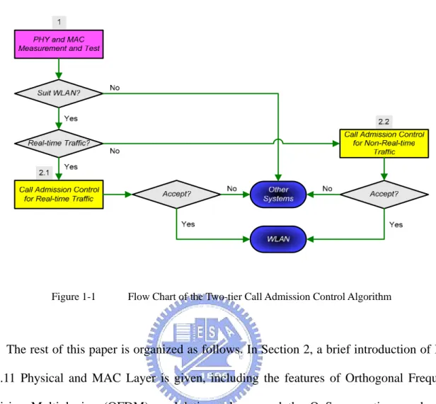
(14) adaptation. [10] discusses the influence of fragmentation sizes, data rates, and power levels on the system performance, and also propose a link adaptation scheme by utilizing two counters for successful and failed transmission, respectively. In [11], it is assumed that the channel is symmetric, which means the Signal to Noise Ratio (SNR) observed at either station is very similar at any time. Therefore, the SNR of the last Acknowledge (ACK) frame could be an indicator of SNR of the other side, and also could be used to select a proper rate. However, Auto Rate Fallback (ARF) algorithm proposed in [12] is the most practical and popular method, hence it is widely used in today’s commercial products. Besides link adaptation, a few Call Admission Control Algorithms have already been proposed in [13] [14] [15]. However, they mainly focus on contention-based MAC mechanism, which provides poor QoS support for real-time traffic. [16] proposes an call admission control algorithm for Variable Bit Rate (VBR) traffic flow. In the algorithm, effective Transmission Opportunity (TXOP) is defined and could be determined by the inversion of packet loss rate expression, yet the calculation is too complicated and impractical in real implementation. Figure 1-1 shows the flow chart of our proposed two-tier call admission control algorithm. In this chart, two distinct viewpoints are taken to analyze the call admission control problem. The first angle is from the single user’s perspective. Since the channel condition of a station may not always be suitable for WLAN system, the station may have some measurements on its channel response and test its capability of connection to WLAN. Label 1 in the flow chart represents this function, which is corresponding to the first tier in the algorithm. The other angle is from the overall system’s perspective, equivalent to the second tier in the algorithm. Since different MAC algorithms are designed to adapt various characteristics of different traffics, it is necessary to have independent Call Admission Control units. This paper categorizes the traffic into real-time and non-real-time traffic, hence we also have distinct metrics to decide whether it is tolerable to accept the requesting stations or not, labeled as 2.1 and 2.2, respectively. 2.

(15) Figure 1-1. Flow Chart of the Two-tier Call Admission Control Algorithm. The rest of this paper is organized as follows. In Section 2, a brief introduction of IEEE 802.11 Physical and MAC Layer is given, including the features of Orthogonal Frequency Division Multiplexing (OFDM) modulation scheme and the QoS supporting mechanisms proposed in the IEEE 802.11e. In Section 3, one of the link adaptation techniques, ARF, and its evolution, Adaptive ARF (AARF), are introduced. In Section 4, the proposed Scheduling concept and algorithm are presented. Also, the Call Admission Control scheme for real-time traffic labeled as 2.1 in Figure 1-1, is described in this section. The simulation scenario and results are presented in Section 5. Finally, this paper makes conclusion in Section 6.. 3.

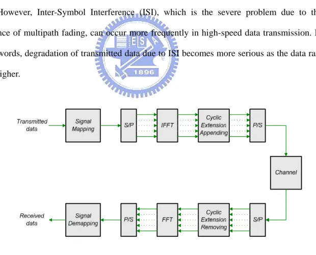
(16) Chapter 2. The IEEE 802.11. 2.1 The IEEE 802.11a PHY. Orthogonal Frequency Division Multiplexing (OFDM), which is a robust multi-carrier modulation technology that has been selected for a number of radio standards including Wireless LAN (IEEE 802.11a,g [17], HiperLAN/2 [18]), DVB-T [19] and Wireless MAN (IEEE802.16a [20]). Figure 2-1 below shows the block diagram of an OFDM system. Using OFDM as the modulation scheme can support few tens or hundreds Mbps of data rate. However, Inter-Symbol Interference (ISI), which is the severe problem due to the existence of multipath fading, can occur more frequently in high-speed data transmission. In other words, degradation of transmitted data due to ISI becomes more serious as the data rate goes higher.. Figure 2-1. OFDM Block Diagram. 4.

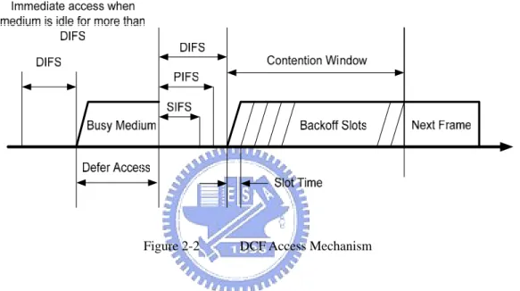
(17) In OFDM, a serial data stream is split into several parallel streams that modulate a group of orthogonal sub-carriers. Compared to the single carrier modulation method, OFDM symbols have a relatively long time duration, but a narrow bandwidth. Therefore, the channel characteristic in OFDM system is changed from a frequency selective fading channel into a frequency flat fading channel. The ISI could be efficiently eliminated by using Guard Interval (GI), which is the tail part of an OFDM symbol and is cyclically placed in front of the symbol. Although GI let the OFDM system being immune against multipath dispersion, the increased symbol duration makes an OFDM system more sensitive to the time variation of mobile radio channels. In particular, the effect of Doppler spreading destroys the orthogonal characteristics between all the sub-carriers, resulting in inter-carrier interference (ICI) due to the power leakage among sub-carriers so that the performance degradation occurs. In [21][22][23][24], the effect of carrier frequency offset, the mathematical expression, and the BER analysis are discussed.. 2.2 The IEEE 802.11 Legacy MAC. The IEEE 802.11 [1] legacy MAC is based on the logical functions called the coordination functions, which determines when a station is permitted to transmit or be able to use the wireless medium. Two coordination functions are defined in legacy IEEE 802.11: the Distributed Coordination Function (DCF) and the Point Coordination Function (PCF).. A.. Distributed Coordination Function (DCF) Distributed Coordination Function (DCF) is the fundamental access method that works. as listen-before-talk scheme, based on a Carrier Sense Multiple Access with Collision Avoidance protocol (CSMA/CA). Before transmitting a frame, a station shall listen to the 5.

(18) radio to check that there is no other transmission in the progress on the wireless medium. However, if more than one station detect the channel as free at the same time, a collision occurs. To avert from this situation, the legacy 802.11 defines a Collision Avoidance (CA) mechanism to reduce the probability of such collisions. That is, before a station delivers MAC Service Data Units (MSDUs) of arbitrary lengths (up to 2304 bytes), it has to keep sensing the channel for an additional random backoff time after detecting the channel as being idle for a minimum duration called DCF InterFrame Space (DIFS). The random backoff time is selected from the range (0, CW-1), where CW is called the contention window. At the first attempt of transmission, CW is assigned to the value CWmin, which is the minimum contention window size. Once the collision occurs, the CW value for the consecutive unsuccessful transmission should be increased up to the maximum value,. CWmax = 2m CWmin , where m is called the maximum backoff stage. The backoff time of each station is decreased as the channel is sensed idle and suspended as the channel is sensed busy. When the medium is sensed idle again, that is, when the prior transmission is completed, the counter is reactivated and continuing to decrease. Only when the counter reaches zero shall a station transmit a frame. Figure 2-2 shows the DCF access operation.. B.. Point Coordination Function (PCF) For supporting time-bounded delivery of data frames, the IEEE 802.11 standard defines. the optional Point Coordination Function (PCF) where the Access Point (AP) grants access to an individual station to the medium by polling the station. Stations can't transmit frames unless the Access Point polls them first. The PCF has higher priority than the DCF, because it may start transmission after a shorter period than DIFS; this time space is called PCF InterFrame Space (PIFS). Besides, the time coordinate always consists of repeated periods,. 6.

(19) called superframes. A superframe starts with a so-called beacon frame, regardless if PCF is active or not, and is composed of a Contention Free Period (CFP) and a Contention Period (CP). During the CFP, the PCF is used for accessing the medium, while the DCF is used during the CP. It is mandatory that a superframe includes a CP of a minimum length that allows at least one MSDU Delivery under DCF.. Figure 2-2. DCF Access Mechanism. The Access Point polls stations according to a polling list, then switches to a contention period when stations use DCF. This process enables support for both synchronous (i.e., video applications) and asynchronous (i.e., e-mail and Web browsing applications) modes of operation.. 2.3 The IEEE 802.11e MAC. The new IEEE 802.11e MAC architecture [25] is conceived as a compatible extension of the legacy IEEE 802.11 MAC. A new Hybrid Coordination Function (HCF) which includes two access schemes is introduced. One of the access schemes is contention-based and is called Enhanced Distributed Coordination Function (EDCF), while the other is polling-based and 7.

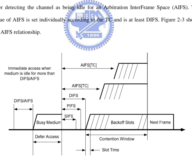
(20) works under the control of Hybrid Coordinator (HC), which is located at the Access Point (AP).. A.. Enhanced Distributed Coordination Function (EDCF) EDCF introduces the concept of Traffic Categories (TCs), which could be considered as. instances of the DCF access mechanism that provides support for the prioritized delivery at the station. MSDUs are now delivered through multiple backoff instances within one station, each backoff instance parameterized with TC-specific parameters. EDCF is operative only during the contention period (CP). In the CP, each TC within the stations independently contends for a Transmission Opportunity (TXOP), which is defined as the interval of time when a specific station can occupy the wireless medium; and each TC also starts a backoff after detecting the channel as being idle for an Arbitration InterFrame Space (AIFS). The value of AIFS is set individually according to the TC and is at least DIFS. Figure 2-3 shows the AIFS relationship.. Figure 2-3. Multiple backoff for different TCs. 8.

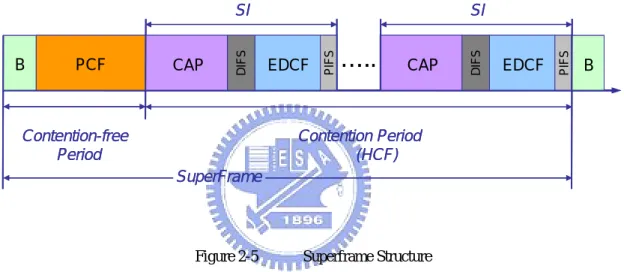
(21) B.. Hybrid Coordination Function (HCF) The HCF extends the EDCF access rules, and its polling mechanism is similar to the. legacy PCF (point coordination function). The time coordinate always consists of repeated periods, called superframe. A superframe starts with a so-called beacon frame, and is composed of a Contention Free Period (CFP) and a Contention Period (CP). The HC, which is called Hybrid Coordinator, is usually located in the Access Point, may allocate TXOPs to itself to initiate MSDUs whenever it wants. However, it is legal only after detecting the channel as being idle for PIFS. Thus, HC gets priority over all other stations in medium access. HCF may be operative during both CP and CFP period. During CP, each station gets its TXOP either when the medium is determined to be available under the EDCF rules or when the station receives a poll frame from HC. During CFP, the TXOP limit is specified by HC in the poll frames. CFP ends by a CF-End frame sent by the HC.. 2.4 HCF Scheduling and Call Admission Control Algorithms. [26] proposes a simple scheduler that can be used as a reference for the future, more complicated schedulers. In this scheduler, a station based on its requirements requests HC for TXOPs: both for its own transmissions as well as transmissions from the AP to itself. Each station that requires contention-free access sends a QoS request frame to the AP containing the mean data rate of the application, the MAC Service Data Unit (MSDU) size and the maximum service interval (MSI) requirements. Upon receiving all requests, the AP chooses the minimum of all MSIs as a value s. Then, the AP calculates the SI that is the sub-multiple of the superframe duration and is lower than the value s. Once the SI is determined, the AP evaluates the different TXOPs allocated to the different flow of all the stations. Figure 2-4 illustrates the arrangement of each TXOP in the simple scheduler.. 9.

(22) TXOP l. TXOP k. TXOP j. TXOP i. TXOP l. TXOP k. TXOP j. TXOP i. TXOP l. TXOP k. TXOP j. TXOP i. SI. SI Figure 2-4. Simple Scheduler. Besides, the superframe in HCF is chopped into several SIs and stations are polled according to a round-robin basis during each SI. Figure 2-5 below shows that after the CFP, EDCF periods and Controlled Access Periods (CAPs) alternate during CP.. Contention-free Period. EDCF. …... CAP. EDCF. PIFS. CAP. DIFS. PCF. SI PIFS. B. DIFS. SI. B. Contention Period (HCF) SuperFrame. Figure 2-5. Superframe Structure. The scheduler calculates the TXOP duration of station j as the maximum of the time to transmit Ni frames at rate Ri and the time to transmit one maximum size MSDU at Ri (plus overheads): n ⎞ ⎛N ×L M TXOPj = ∑ max ⎜⎜ i i + O, + O ⎟⎟ Ri i =1 ⎠ ⎝ Ri. (2-1). ⎡ SI × ρ i ⎤ Ni = ⎢ ⎥ ⎢ Li ⎥. (2-2). i = 1..n. where, n. - Number of individual traffic streams within a station. ρ. - Mean Application Data Rate 10.

(23) L. - Nominal MSDU Size from the negotiated TSPEC. SI. - The Scheduled Service Interval. R. - Physical Transmission Rate. M - Size of Maximum MSDU, i.e., 2304 bytes O. - Overheads in time units. Admission Control is trivial with the Simple Scheduler. The total fraction of transmission time reserved for contention-free transmission (CAP reservation, CR) for m stations at any given moment can be easily calculated as follows: m. TXOPj. j =1. SI. CR = ∑. (2-3). In order to check if a new traffic stream can be accepted, the HC only needs to check if the new TXOP for traffic stream k plus the current CR is lower than or equal to the maximum fraction of time that can be spent by contention-free bursts (the normalized CAP rate):. T − TCP TXOPk + CR ≤ T SI. (2-4). where T indicates the superframe interval and TCP is the time used for EDCF access.. 11.

(24) Chapter 3. ARF and AARF Algorithms. 3.1 ARF Introduction. Rate adaptation is the process of dynamically switching the transmission rate to match with the varying channel conditions. Stations adapt their transmission rate to achieve the optimum throughput for their given channel conditions. ARF (Auto Rate Fallback) [12] was the first rate adaptation algorithm to be published. In ARF, the sender selects the best rate based on information from previous data packet transmissions. Specifically, the ARF algorithm decreases the current rate and starts a timer when two consecutive transmissions fail in a row. When either the timer expires or the number of successfully received per-packet acknowledgments reaches 10, the transmission rate is increased to a higher data rate and the timer is reset. When the rate is increased, the first transmission after the rate increase (commonly referred to as the probing transmission or probing packet) must succeed or the rate is immediately decreased and the timer is restarted rather than trying the higher rate again.. 3.2 Proposed two-dimensional ARF Markov Chain. In the proposed call admission control, we pay more attention to the transition between mode and mode (the changing of rates) because the value of the rate could influence the efficiency of wireless resource utilization. Unless the medium utilization is controlled exquisitely, the call admission control could not guarantee the accepted incoming user’s quality of service. In order to calculate the switching probabilities between mode and mode,. 12.

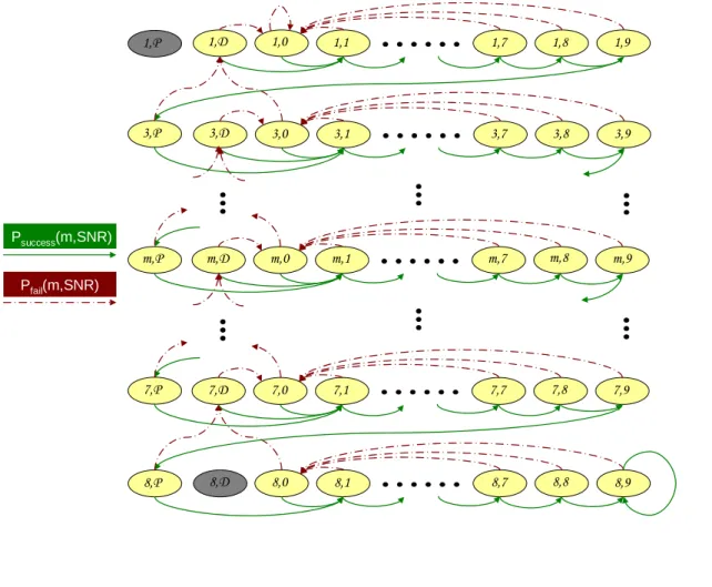
(25) we derive a two-dimensional Markov chain from the ARF steps described above and provide the analytical mathematical models for this problem. The proposed two-dimensional ARF Markov chain is shown in Figure 3-1, and it completely presents the behavior and proceedings of ARF. The first parameter of each state indicates the current mode from 1 to 8 in IEEE 802.11a, corresponding to transmission rate 6M, 9M, 12M, 18M, 24M, 36M, 48M and 54M. (Note that mode 2 is skipped since the performance of mode 2 is always poorer than that of mode 3.) The second parameter describes the historical transmission record. P indicates that the station has already completed the consecutive 10 successful transmissions and is going to send the probing packet. D suggests that the transmission rate is just decreased due to two consecutive transmission fails. Moreover, the numerals 0~9 indicates the number of consecutive successful transmissions. Note that the real and the dash lines represent the successful and the failed transmission of a packet, respectively. The calculation of the packet error probability could be referred to [9]. Our intention is to derive the transition probability between each mode from the proposed two-dimensional Markov chain, including transit-down probability, Pdown, and transit-up probability, Pup. The calculations are as follows:. Pdown m = P (m − 1 | m ) =. P (m − 1 ∩ m ) P (m ). ⎡9 ⎤ 2 Pf (m, SNR ) × ⎢∑ b(m, k ) + b(m, D )⎥ + Pf (m, SNR ) × [b(m, P ) + b(m,0 )] ⎣ k =1 ⎦ = 9 ∑ b(m, k ) + b(m, P ) + b(m, D ). (3-1). k =0. Pupm = P (m + 1 | m ) =. =. Ps. 10. P (m + 1 ∩ m ) P (m ). (m, SNR ) × [b(m, P ) + b(m, D ) + b(m,0)] + ∑ (Ps10 −k (m, SNR ) × b(m, k )) 9. k =1. 9. ∑ b(m, k ) + b(m, P ) + b(m, D ) k =0. 13. (3-2).

(26) where m. - the current mode of the station. b. - the state probability. Ps. - the successful transmission probability of a packet. Pf. - the failed transmission probability of a packet. 1,P. 1,R 1,D. 1,0. 1,1. 1,7. 1,8. 1,9. 3,P. 3,R 3,D. 3,0. 3,1. 3,7. 3,8. 3,9. m,P. i,R m,D. m,0. m,1. m,7. m,8. m,9. 7,P. 7,R 7,D. 7,0. 7,1. 7,7. 7,8. 7,9. 8,P. 8,R 8,D. 8,0. 8,1. 8,7. 8,8. 8,9. Psuccess(m,SNR) Pfail(m,SNR). Figure 3-1. ARF Markov Chain. 14.

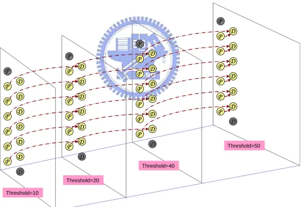
(27) 3.3 AARF Introduction. Although ARF is reasonable good at handling the short-term variation of the wireless medium characteristics in an infrastructure network, it fails to handle efficiently while the channel conditions keep quite stable. When the channel does not change at all, ARF will still try to use a higher rate every 10 successfully transmitted packets. Obviously, the rate raising behavior actually makes no sense and the number of retransmissions will increase resulting in the deterioration of the effective throughput. AARF [27] deals with this situation by using an exponentially increased threshold, which is used to decide when to increase the current rate. Instead of using a fixed value of 10, the threshold in AARF becomes 10, 20, 40, and 50 (maximum bound). The proceedings of AARF are similar to those of ARF except the following steps. First, when the transmission of the probing packet fails, not only is the rate switched to the previous lower one (as in ARF), but also the threshold is multiplied by two (with a maximum bound set to 50). Moreover, the threshold should be reset to its initial value of 10 when either the rate is decreased due to two consecutive failed transmissions, or when the transmission of probing packet succeeded.. 3.4 Proposed three-dimensional AARF Markov Chain. Again, it is paid much attention to obtain the transition probabilities of each mode. Therefore, we have done the same thing to AARF algorithm, that is, to derive the corresponding Markov chain. The Markov chain of AARF becomes to three-dimension now. The first and the second dimension are just the same as ARF and the third dimension indicates the different thresholds. Since it will become a mess if the complete three-dimensional behavior of AARF is plotted; here, only the differences between ARF and AARF are shown. The first difference is that when the transmission of the probing packet fails, not only is the 15.

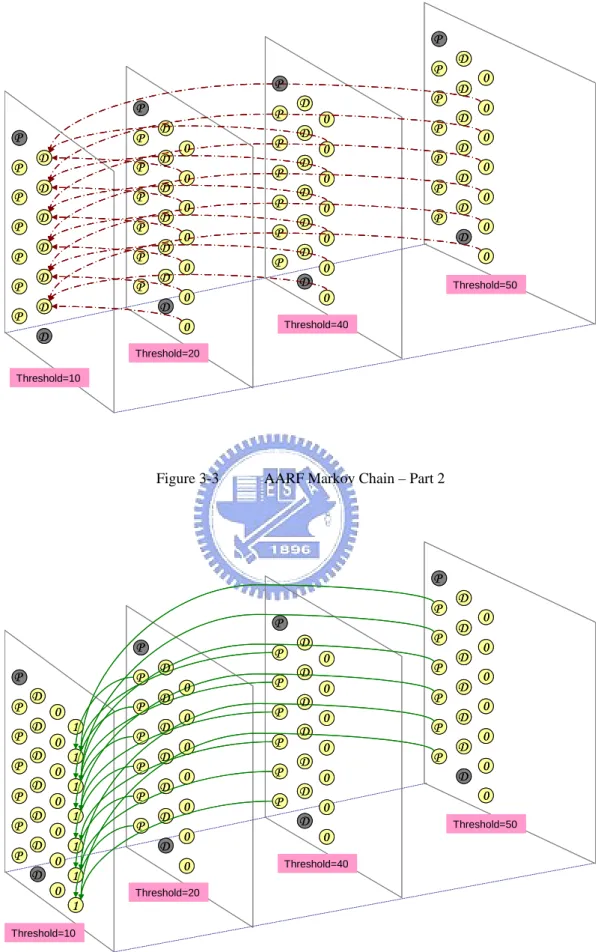
(28) rate switched to the previous lower one (as in ARF), but also the threshold is multiplied by two. Figure 3-2 illustrates this behavior. Besides, there are two situations when the threshold should be reset to its default value. Figure 3-3 illustrates the first one that when the rate is decreased due to two consecutive failed transmissions, the threshold becomes 10. And Figure 3-4 shows that when the transmission of probing packet succeeded, the threshold should also be reset. Once the AARF Markov chain is obtained, it is feasible to calculate each state’s steady probability. And with these state probabilities, we could calculate the transit-down probability (Pdown) and transit-up (Pup) probability for each mode under various SNR values, similar to those that have been done to ARF. These two parameters become important keys while designing Call Admission Control algorithm for real-time traffic, and we show each of the calculations below. In the following section, there will also be some discussions about how they play their roles.. Pdown m = P (m − 1 | m ) =. P (m − 1 ∩ m ) P (m ). ⎧⎪ 2 ⎡Td −1 ⎤ ⎪⎫ ( ) P m , SNR × ⎨ f ∑ ⎢ ∑ b(m, k, d ) + b(m, D, d )⎥ + Pf (m, SNR ) × [b(m, P, d ) + b(m,0, d )]⎬ ⎪⎭ d =1 ⎪ ⎣ k =1 ⎦ ⎩ = Td −1 4 ⎫ ⎧ ⎨ ∑ b(m, k, d ) + b(m, P, d ) + b(m, D, d )⎬ ∑ d =1 ⎩ k = 0 ⎭ 4. (3-3). Pupm = P (m + 1 | m ) =. P (m + 1 ∩ m ) P (m ). ⎧Ps10 (m, SNR ) × b(m, P, d ) + PsTd (m, SNR ) × [b(m, D, d ) + b(m,0, d )] + ⎫ ⎪T −1 ⎪ ⎨d ⎬ ∑ Td − k (m,SNR ) × b(m, k, d ) d =1 ⎪ ∑ Ps ⎪ ⎩ k =1 ⎭ = Td −1 4 ⎫ ⎧ ⎨ ∑ b(m, k , d ) + b(m, P, d ) + b(m, D, d )⎬ ∑ d =1 ⎩ k =0 ⎭ 4. (. ). 16. (3-4).

(29) where m. - the current mode of the station. b. - the state probability. Ps. - the successful transmission probability of a packet. Pf. - the failed transmission probability of a packet. d. - the corresponding value of the third dimension. Td. - the corresponding value of threshold. P P. P P P P P P P P P. P D D D D D D. P P P P P. D D D D D D. P P P P P P. D. P. D. P. D. P. D. P. D. P. D D. D Threshold=40. D Threshold=20 Threshold=10. Figure 3-2. AARF Markov Chain – Part 1. 17. D D D D D D D. Threshold=50.

(30) P P. P P P P P P P P P. P D. P. D. P. D. P. D. P. D. P. D D D D D D D. D. P 0. P. 0. P. 0. P. 0. P. 0. P. D D D D D D. 0. 0 0 0 0. P P P P. D D D D D D. 0. 0 0 0 0 0 0 0. 0. Threshold=50. 0. 0. D. P. D. D. Threshold=40. Threshold=20 Threshold=10. Figure 3-3. AARF Markov Chain – Part 2. P P. P P P P P P P P P. P D D D D D D D. 0 0 0 0 0 0 0. P 1 1 1 1 1 1. P P P P. P. D D D D D D D. 0. P. 0. P. 0. P. 0. P. 0. P. D D D D D D. 0 0. P. D 0 0 0 0. P P P P. 0 0 0. Threshold=40. Threshold=20. 1. Threshold=10. Figure 3-4. AARF Markov Chain – Part 3 18. D D D D D D D. 0 0 0 0 0 0 0. Threshold=50.

(31) Chapter 4. Proposed Scheduling and Call Admission Control Algorithm. 4.1 Proposed Scheduling Algorithm. From section 2.4, it is noticed that there are still a few flaws in simple algorithm. The simple algorithm is intended as a reference only and it just respects the minimum requirements; so, it is somehow inefficient. First, the TXOP duration of each station is always the same and corresponds to the transmission time of an M-sized (maximum MSDU size, i.e., 2304 bytes) packet at a certain PHY rate. While this may be suitable for traffic types that present small bursts of constant size (e.g., voice over IP, VoIP), some traffic types like MPEG-4 video present bursts of variable size formed by several packets (e.g., an MPEG-4 I-frame is usually much larger than a P-frame or B-frame). In other words, these types of traffic have various packet sizes and various packet inter-arrival times. With the simple algorithm, transmission of a long burst packet can lead to significant transmission delay, even cause packet drop. While for packet whose size is much smaller than M, TXOP calculation is too conservative so that waste of wireless resource becomes more severe. Moreover, the adoption of rate adaptation technique is not taken into consideration in simple algorithm either. Stations under continuous changing channel are using different transmission rate, hence they ought to occupy different TXOP from time to time. Real-time scheduling theory has already proven that Earliest Deadline First (EDF) or Earliest Due Date (EDD) is optimal in a wide set of real-time scheduling problems [28][29]. For this reason, EDD is chosen to be the framework of our scheduling method. Besides, two. 19.

(32) different concepts should be introduced when we design the EDD-based scheduler. They are discussed as follows, respectively.. . Approach one Before a station is allowed to use the medium, a polling message should be broadcasted. and this message is regarded as an overhead. Approach one in scheduler design allows a station to transmit multiple packets for one poll. The simple algorithm we have introduced belongs to this kind of approach. Obviously, this approach maximizes the system capacity due to the minimization of the amount of overhead. Besides, after a certain station is polled and the first packet in its buffer (or the most urgent packet) is delivered, the remaining packets could be delivered consecutively without other polls. It results in the situation that the time occupied by those remaining packets might retard the process of other stations’ packets, which may be more urgent, from making themselves on time. Therefore, the disadvantage of this approach is that packet loss rate might suffer from the negative impact. Approach one allows multiple packet transmissions. But what should the number of packets that is granted for one poll be? We suggest that it could be equal to the total amount of data in the buffer. People might wonder if there is a situation that the amount of data in the buffer is too much and it takes such a long time to complete all of their transmission, so that all packets from other stations will be dropped because of missing deadlines. Actually, we do not have to worry about this situation, because with our properly designed CAC (Call Admission Control) Algorithm, it will never happen. In other words, this issue is addressed in the proposed CAC algorithm, and each station’s QoS would be achieved not by the scheduler, but by the proposed CAC algorithm. The detailed discussion of the proposed CAC will be presented in the next section.. 20.

(33) Back to the scheduler design approach one, TXOP for a station depends on the total amount of data and the current physical transmission rate. Hence the TXOP calculation for traffic stream j becomes to:. ⎛ ⎡n ⎞ +l ⎤ TXOPj = ∑ ⎜ ⎢ overhead j ,k ⎥ • Tsym + Toverhead ⎟ ⎜ ⎢ BpS (m j ) ⎥ ⎟ k =1 ⎝ ⎣ ⎦ ⎠ Np. (4-1). where Np indicates the number of packets in the buffer; noverhead is the total amount of PHY and MAC header and tail (in terms of byte); lj,k is the size of the kth packet of traffic stream j. Toverhead present as the time spent on polling, acknowledgement, and SIFS (Short InterFrame Space). Tsym is the symbol time, e.g., 4us in IEEE 802.11a standard. BpS(mj) stands for Byte-per-Symbol information for PHY mode mj and its values are given in Table 4-1. The capacity performance could be even better when Packet Concatenation (PAC) protocol [30] is adopted. This technique intends to make multiple MAC packets to share the same control messages, which are Physical Layer Convergence Protocol (PLCP) preamble, PLCP header, and the tail. Since these control messages are always BPSK modulated, which is the most conservative way, the wasted on wireless resources for these messages is quite large. Multiple MAC packets sharing the same control message further reduces the amount of overhead. Last, if PAC protocol is utilized in our scheduler design approach one, the TXOP calculation for traffic stream j becomes to: Np ⎤ ⎡ ⎢ noverhead + ∑ l j ,k ⎥ k =1 ⎥ • Tsym + Toverhead TXOPj = ⎢ ⎢ BpS (m j ) ⎥ ⎥ ⎢ ⎦ ⎣. . (4-2). Approach two On the other hand, the second approach allows only one packet transmission for a single. poll. Unlike approach one which takes only the first packet’s delay bound in each station’s buffer as the metric of scheduling priority, in approach two, each packet’s delay bound is 21.

(34) treated as the same, no matter what station they belong to. Therefore, the information is more sufficient and the schedule arrangement will be more precisely. This behavior has an influence which is just opposite to that of approach 1: larger overhead, smaller capacity, but better packet loss performance. The formula for TXOP in approach two is shown below.. ⎡n + l j ,1 ⎤ TXOPj = ⎢ overhead ⎥ • Tsym + Toverhead ⎣⎢ BpS (m j ) ⎦⎥. (4-3). where lj,1 indicates the size of the traffic stream j’s first packet, or the size of the most urgent packet, in the traffic stream j’s buffer.. Table 4-1. Mode dependent parameters of IEEE 802.11a PHY [1] Code bits. Data rate Mode (Mb/s). Coding. Code bits. rate. per subcarrier. (R). (NBPSC). Modulation. Data bits. Data bytes. per OFDM per OFDM per OFDM. scheme. symbol. symbol. symbol. (NCBPS). (NDBPS). (BpS). 1. 6. BPSK. 1/2. 1. 48. 24. 3. 2. 9. BPSK. 3/4. 1. 48. 36. 4.5. 3. 12. QPSK. 1/2. 2. 96. 48. 6. 4. 18. QPSK. 3/4. 2. 96. 72. 9. 5. 24. 16-QAM. 1/2. 4. 192. 96. 12. 6. 36. 16-QAM. 3/4. 4. 192. 144. 18. 7. 48. 64-QAM. 2/3. 6. 288. 192. 24. 8. 54. 64-QAM. 3/4. 6. 288. 216. 27. 22.

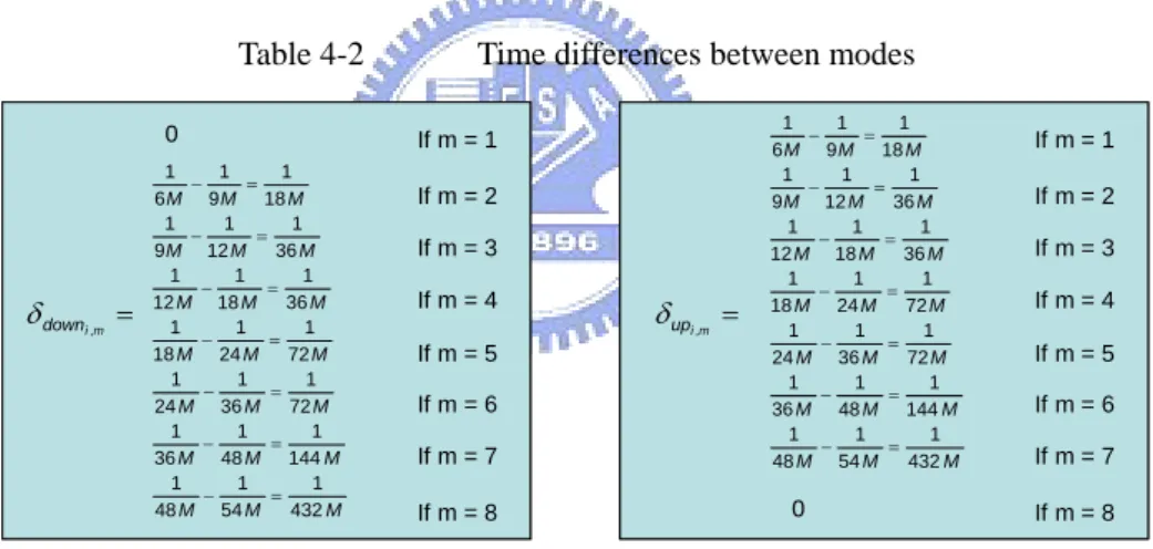
(35) 4.2 Proposed Call Admission Control Algorithm for Real-time Traffic. In this section, the second tier call admission control algorithm for real-time traffic is presented. It is mentioned before that the scheduler should be designed to have more flexibility because the characteristics of certain traffics are quite unstable. This concept should also be introduced in Call Admission Control Algorithm. Each TXOP now is a varying value, and the duration between two polls of a station is changing also. Therefore, in order to fulfill the Delay Bound (DB) requirement of each traffic stream, we bring up an idea of adaptive “buffer time” (BT) to compensate the variation of each TXOP. A few parameters introduced in our Call Admission Control algorithm are defined as follows. And we suggest checking Figure 4-1 while reading the definitions. ¾. SI. (Service Interval). SI = min(DBi ). ∀i. (4-4). SI is set as the smallest Delay Bound (DB) among all traffic streams. ¾. G (Summation of each TXOP) k. G = ∑TXOPi. (4-5). i =1. G indicates the total amount of time occupied by all stations within a SI interval. ¾. BT (Buffer Time) k. (. ). BT = ∑ Ni × Li × Pdowni ,m × δ downi ,m − Pupi ,m × δ upi ,m + ∆ i =1. (4-6). Ni and Li are as same as the definitions in the simple algorithm. Just like the description above, BT is a period of time in order to compensate the variation of each station’s TXOP. In section 3, we have already discussed the rate adaptation technique, AARF, which traces the channel condition continuously to achieve the maximum effective throughput. For each station under a certain SNR value, there is a corresponding transit-down and transit-up probability, denoted as Pdown and Pup respectively. Moreover, while the mode increases or decreases, there will be a 23.

(36) time difference even for a fixed amount of data. Table 4-2 shows these time differences compliant to IEEE 802.11a. δ down denotes the time difference for one bit when mode decreases, and δ up denotes that when mode increases. The last term, ∆, intends to compensate the unpredictable characteristics of each traffic stream, especially for variable bit rate (VBR) traffic. Although Traffic Specification (TSPEC) provides some traffic statistics (e.g. user priority, maximum MSDU size, mean data rate, etc), VBR traffic usually does not follow this feature exactly. Hence we add a ∆ in BT calculation to reserve an extra period of time in order to balance this unstable property. By combining the parameters described, BT is able to accommodate the timing variation caused by rate adaptation and variation of the packet size and packet inter-arrival time.. Table 4-2 0. δ down. ¾. i ,m. =. 1 1 1 − = 6 M 9 M 18 M 1 1 1 − = 9 M 12 M 36 M 1 1 1 − = 12 M 18 M 36 M 1 1 1 − = 18 M 24 M 72 M 1 1 1 − = 24 M 36 M 72 M 1 1 1 − = 36 M 48 M 144 M 1 1 1 − = 48 M 54 M 432 M. Time differences between modes If m = 1 If m = 2 If m = 3 If m = 4. δ up. If m = 5 If m = 6 If m = 7. i ,m. =. 1 1 1 − = 6 M 9 M 18 M 1 1 1 − = 9 M 12 M 36 M 1 1 1 − = 12 M 18 M 36 M 1 1 1 − = 18 M 24 M 72 M 1 1 1 − = 24 M 36 M 72 M 1 1 1 − = 36 M 48 M 144 M 1 1 1 − = 48 M 54 M 432 M. 0. If m = 8. If m = 1 If m = 2 If m = 3 If m = 4 If m = 5 If m = 6 If m = 7 If m = 8. Deadline Deadline = SI − BT. (4-7). Deadline is the boundary we set to detect whether the system still has the ability to compensate the expansion of each TXOP. If the summation of each TXOP, G, exceeds the Deadline, it implies that G in the next SI interval might goes beyond the SI, which is the smallest Delay Bound. This means packet drop will occur and the performance will degrade.. 24.

(37) G>Deadline. Deadline DBmin. Red Alert!!!!!! if RD <= Nreject n=n+1;. TXOP l. TXOP k. TXOP j. TXOP i. BT. else. Deadline DBmin. Reject All Request! SI l. TXOP. TXOP k. TXOP i. BT. Deadline. SI. TXOP m. TXOP l. k. TXOP. TXOP is various in each SI. TXOP j. BT TXOP i. Note:. DBmin. SI. Figure 4-1. Scheduling and Call Admission Control Algorithm. It should be noticed that, at the beginning of each SI interval, Pdown and Pup should be updated according to each station’s previous SNR; and the Buffer Time, BT, should also be updated to a new value. Once G is greater than Deadline, it implies that at the next SI interval, G has a certain probability to exceed SI because of the decrease of transmission rate, hence cause packet drops. Besides the four parameters, a counter n also shows up. Once the summation of each TXOP (G) goes beyond the Deadline, n should add itself by 1. Another parameter called “Reject Density”, RD, is defined as n divided by the observation interval (in terms of second). It implies the density of budget violation (G>Deadline) in a certain time duration. If RD is greater than a pre-defined value, Nreject, the incoming traffic should be rejected. Recall that for handoff design in UMTS [31], there is a hysteresis along with a timer in order to avoid ping-pong effect. This is the concept to avoid sudden change of a station’s SNR. RD in our 25.

(38) algorithm shares the same idea and further extends its function to accommodate different required Packet Loss Rate (PLR). Obviously, if the requirement of PLR is loose, Nreject could be set larger and allows higher Reject Density, and vice versa. This concept and the proper setting of Nreject will be discussed in section 5.2. In conclusion, the criterion to decide whether a new traffic stream could join the system or not is: if. (G > Deadline ) ∩ (RD > Nreject ). Î Reject. (4-8). Recall that in scheduler design in the previous section, approach one allows multiple packet transmissions. And we suggest that the number of packets that is granted for one poll could be the total amount of data in the buffer. People might wonder if the amount of data in the buffer is too much and it takes such a long time to complete all of their transmission, so that all packets from other stations will be dropped because of missing deadlines. Actually, we do not have to worry about this situation. In our CAC algorithm, a parameter SI (Service Interval) is introduced and equals to the smallest Delay Bound among all traffic streams. Combining the scheduler and the corresponding call admission control, it is guaranteed that a traffic stream will be polled at least once per SI, and the amount of data accumulated in the buffer during SI should within a certain range, which we have already taken into consideration. In other words, we achieve each station’s QoS by the proposed CAC algorithm, but not scheduler.. Note:. It is obvious that the Call Admission Control described above corresponds to the. scheduler design approach one, which allows transmitting multiple packets per poll. To accommodate approach two, the only modification required in our CAC algorithm is to replace the SI by the lowest mean value of packet inter-arrival time, and substitute Ni in BT calculation for 1.. 26.

(39) Chapter 5. Simulation Results. IEEE 802.11a is adopted as the background in the following simulations. The critical parameters that have been defined in IEEE 802.11a standard and have been used in the simulations are concluded in Table 5-1 to make it clear.. Table 5-1. IEEE 802.11a parameters [1]. Parameter. Value. NSD: Number of data subcarriers. 48. NSP: Number of pilot subcarriers. 4. NST: Number of subcarriers, total. 52 (NSD + NSP). ∆F: Subcarrier frequency spacing. 0.3125 MHz (=20MHz/64). TFFT: IFFT/FFT period. 3.2 µs (1/∆F). TSlot: Slot time. 9 µs. TSIFS: SIFS time. 16 µs. TDIFS: DIFS time. 34 µs (=TSIFS + 2×TSlot). CWmin: minimum contention window size. 15. CWmax: maximum contention window size. 1023. TPREAMBLE: PLCP preamble duration. 16 µs (TSHORT+ TLONG). TSIGNAL: Duration of the SIGNAL BPSK-OFDM symbol. 4.0 µs (TGI + TFFT). TGI: Guard interval duration. 0.8 µs (TFFT / 4). TGI2: Training symbol guard interval duration. 1.6 µs (TFFT / 2). TSYM: Symbol interval. 4 µs (TGI + TFFT ). TSHORT: Short training sequence duration. 8 µs (10 × TFFT / 4 ). TLONG: Long training sequence duration. 8 µs (TGI2 + 2 × TFFT). 27.

(40) 5.1 IEEE 802.11a PHY Simulation Results. In this section, the first tier of the proposed Call Admission Control Algorithm, which refers to the function unit “PHY and MAC Measurement and Test” labeled as 1 in Figure 1-1, is evaluated. IEEE 802.11a uses OFDM and supports eight different data rates or eight different modes, ranging from 6 Mbps to 54 Mbps. Four modulation schemes, BPSK, QPSK, 16QAM, 64QAM, along with two convolution coding rates, 1/2 and 3/4, form these eight modes. Besides, in each communication system, it is always crucial to inspect the transmission reliability, and Bit Error Rate (BER) is one of the metrics that is commonly used to determine the performance of a certain communication system. In this study, we simulate the BER performance of the four modulation schemes mentioned above not only under AWGN, but also under different Rayleigh fading channels with moving speed equals to 2m/s, 10m/s, 20m/s, and 50m/s, respectively. The following figure (Figure 5-1) shows the simulation results. As it is mentioned before, OFDM system is sensitive to the time variation of mobile radio channels. Therefore, once the fading process becomes more severe, the performance degrades significantly. From the results, we observed that when the channel is not stable, it is not appropriate to select 16QAM or 64QAM as the modulation scheme at all. It is also concerned that for different fading channels, the throughput performance will change dramatically due to degraded BER performance. Figure 5-2 shows the simulation results for Mode1 to Mode4 under AWGN, Rayleigh fading channel with moving speed equals to 2m/s, 10m/s, 20m/s, and 50m/s. Here the performances for Mode5 to Mode8 are not shown because Rayleigh fading makes all these throughputs zero. This consequence has just matched the simulation results in Figure 5-1, which displayed that the BER for 16QAM and 64QAM approach to 0.5, hence no throughput could be obtained.. 28.

(41) (a). (b). (c). Figure 5-1. (d). BER vs. Eb/No. (a) BPSK (b) QPSK (c) 16QAM (d) 64QAM. 29.

(42) (a). (b). (c). (d). Figure 5-2. Throughput under different fading channels. (a) Mode1 (b) Mode2 (c) Mode3 (d) Mode4. Except BER performance, throughputs of each mode in IEEE 802.11a under DCF MAC mechanism are also simulated, as shown in Figure 5-3. In the simulation, AWGN environment and 2000 bytes payload size are assumed when calculating the throughputs. Obviously, if rate adaptation is adopted, the maximum throughput could be achieved while SNR value is varying.. 30.

(43) Figure 5-3. Link Adaptation. Since DCF is a contention based access mechanism, it is apparent that when the number of users increases, the collision probability also raises. Figure 5-4 shows this consequence. Moreover, the impact from number of users is shown in Figure 5-5 and Figure 5-6. As predicted, the throughput performances degrade gradually while the loading becomes heavier, resulting from the higher collision probability. The curves from top to down in Figure 5-5 (a) and Figure 5-6 (a) represent the throughputs for number of users from 1 to 20 under different SNRs. Besides, the individual saturation throughputs from number of users 1 to 200 are picked out and associate with each other to emphasize the influence of number of users. Figure 5-5 (b) and Figure 5-6 (b) illustrate this effect.. Figure 5-4. Collision Probability 31.

(44) (a) Figure 5-5. (b). Mode1~4 (a) Individual throughput for number of users 1~20 (b) Individual saturation throughput. 32.

(45) (a) Figure 5-6. (b). Mode5~8 (a) Individual throughput for number of users 1~20 (b) Individual saturation throughput. 33.

(46) 5.2 Proposed CAC Algorithm for Non-real time Traffic. From Figure 5-4, it is observed that when number of users increases, the collision probability becomes higher. This phenomenon results in larger inter-packet delay and smaller channel utilization. Although delay is usually not a great issue when dealing with non-real time traffic, there are still some delay constraints for certain of specific applications. Taking TCP for example, the delay between the packet transmitting and the acknowledgement receiving should be within the value of Retransmission Timeout (RTO), or the control unit would regard this as network congestion and retransmit the data segment. Therefore, the objective of CAC for non-real time traffic would not only to maximize the throughput and the number of granted users, but also to satisfy the delay constraints. Figure 5-7 shows the relationship between the average inter-packet delay and the collision probability. It is straightforward that when collision probability is larger, the user would have to wait longer to get the medium. The wasting time results from the collision instances and the repetition of DCF MAC backoff mechanism as described in section 2.2 and 2.3.. Mode1 Mode8. Figure 5-7. Average Inter-packet Delay vs. Collision Probability. 34.

(47) The channel utilization is also provided. Figure 5-8 shows its relation with the average inter-packet delay. Obviously, the trend is very similar with that in Figure 5-7, which would have an exponential growth. It is observed in Figure 5-8 that when the channel utilization is about lower than 15%, the delay would increase dramatically. Therefore, the operation range for the CAC control may around 10%~20% for the channel utilization and the corresponding value of the average inter-packet delay is about 10. Under this condition, the collision probability is around 0.8 and the supporting number of users is around 150 according to Figure 5-7 and Figure 5-4, respectively.. Mode1. Mode8. Figure 5-8. Average Inter-packet Delay vs. Channel Utilization. 35.

(48) 5.3 Proposed Scheduling and CAC Algorithm for Real-time Traffic. In this section, the performances of the proposed Scheduling and Call Admission Control Algorithms are evaluated. Actually, it matches with the function unit “Call Admission Control for Real-time Traffic”, which is labeled as 2.1 in Figure 1-1.. A.. Simulation Models and Traffic Parameters The platform in the following simulations is modeled as an infrastructure network, where. the scheduler resides in the AP and arranges the order of each transmission. Besides, two types of real-time traffic are taking into concern in this study to evaluate the proposed algorithm. One of the traffic is an audio source which is suitable to G.729A [32]. The mean data rate and the nominal MSDU size are 24 kb/s and 60 bytes, respectively. For video source, the traffic statistics of a real MPEG-4 streaming (Lecture Room-Cam video stream [33]) generated by “Video Traces Research Group” is used and the delay bound is set as 120 ms. The parameters of both traffics involved in the simulation are listed in Table 5-2. To compare the performances between the simple algorithm (TGe algorithm) and the proposed algorithm, three important metrics are defined as follows: ¾. Packet Loss Rate (PLR):. the fraction of packets that have been dumped since the. delivery time exceeds the corresponding delay bound. ¾. Mean Delay: the average time interval between the arrival and the delivery time of a packet.. ¾. Jitter Delay: the standard deviation of the delay.. Note that the packets that have already been dropped are excluded from the calculations of mean delay and jitter delay. Hence both values only reflect to the performances caused by the valid packets.. 36.

(49) Table 5-2. B.. Traffic parameters for VoIP and video. Service. VoIP (G.729A). Video (MPEG-4). Mean data rate. 24 kb/s. 630 kb/s. Nominal MSDU size. 60 bytes. 1024 bytes. Maximum MSDU size. 60 bytes. 1024 bytes. Mean inter-arrival time. 20 ms. 13 ms. Delay bound. 60 ms. 120 ms. Simulation Results Three Scenarios are established in the simulation. For each of them, mixed traffic. environment is considered, including a fixed number of VoIP traffics (set as 30) and a gradually increasing number of MPEG traffics. Besides, the channel conditions and the traffic characteristics are set differently in each scenario. Scenario 1 is determined as the simplest case while the scenario 3 is the most complex one. The detail descriptions of them will be discussed in the following paragraphs, respectively.. ¾. Scenario 1 The first scenario considers fixed transmission mode (i.e. fixed bandwidth) for each. station, which is mode 5 (24 Mbps). It also assumes that both the VoIP and MPEG traffic are Constant Bit Rate (CBR) for simplicity. The simulation result of the Packet Loss Rate is shown in Figure 5-9. The mean delay and jitter delay for VoIP and MPEG traffic are depicted in Figure 5-10 and Figure 5-11, respectively. It is obvious in Figure 5-9 that the proposed algorithm could support up to 50 total amount of traffic streams (30 VoIP traffics plus 20 MPEG traffics) without any packet loss, while only 43 traffic streams (30 VoIP traffics plus 13 MPEG traffics) are granted by using the simple algorithm. Note that since the TXOPs for 30 VoIP traffic are reserved, the packet loss 37.

(50) rate for VoIP is zero. Hence the line of simple algorithm only shows the PLR of the MPEG traffic. Because in the simple algorithm, the packet size of VoIP traffic is much less than M (2304 bytes) in equation (2-1), the actual demanding transmission duration is less than what has been reserved. Therefore, the reduction of capacity in the simple algorithm results from the conservative TXOP duration assigning.. Figure 5-9. Packet Loss Rate in Scenario 1. In Figure 5-10, the mean delay and jitter delay performances of the simple algorithm for VoIP traffic are keeping about a certain value. The reason is that for those existing 30 traffic streams, TXOPs have already been reserved no matter whatever MPEG traffic comes in, just like Figure 2-4 shows. In other words, although the congestion happens (equation (2-4) holds) while the number of MPEG traffics achieves 14, this would not influence the reservation of each TXOP for those existing traffic. (Recall that the packets that are dropped are excluded from the calculations of mean delay and jitter delay, hence the negative impact results from increasing number of traffics only exhibits in the packet loss rate performance, shown in Figure 5-9 ). However, the proposed algorithm is not based on the reservation manner, but EDD manner, which indicates that the medium is occupied by the traffic having the earliest due date. As the total number of traffics increases, it becomes more and more difficult for one 38.

(51) traffic stream to obtain the medium, no matter VoIP traffic or MPEG traffic it is. Therefore, the mean delay and jitter delay have an increasing trend while the loading becomes heavier.. (a). Figure 5-10. (b). (a) Mean Delay (b) Jitter Delay for VoIP traffic in Scenario 1. The performances of MPEG traffic are depicted in Figure 5-11. The trend of each performance for simple algorithm is very similar to that of VoIP traffic shown in Figure 5-10, which is, keeping a certain value roughly before the system becomes congested (30 VoIP traffics plus 14 MPEG traffics in this case). The metrics of the proposed algorithm behaves as an increasing manner and it shares the same reason as explained in the previous paragraph. It should be noticed that the mean delay and jitter delay for VoIP traffic are very close to those for MPEG traffic in the simple algorithm (Mean delay ≈ 30 ms, jitter delay ≈ 17.5 ms). However, the proposed EDD based scheduler makes “Service Differentiation” and provides different delay levels to different services types. This difference is due to that the EDD scheme will differentiate user priorities based on the delay requirements. Besides, the mean delay and jitter delay of MPEG traffic in the simple algorithm are a little smaller than those of the proposed algorithm. This could be seen as the compensative consequences of the large. 39.

(52) reduction of mean delay and jitter delay for VoIP traffics (refer to Figure 5-10 (a) and Figure 5-10 (b)). Therefore, the overall delay performances of the proposed algorithm still outperform those of the simple algorithm.. (a). Figure 5-11. (b). (a) Mean Delay (b) Jitter Delay for MPEG traffic in Scenario 1. It is worth emphasizing that the scenario 1, which stands for fixed bandwidth and CBR, is the best condition for the simple algorithm. It perfectly matches the assumption while designing the length of the fixed TXOP duration (equation (2-1)). Unfortunately, scenario 1 is not practical in the real situation, which adopts link adaptation and also considers VBR traffic. Therefore, if the simulation is under a more realistic environment, it is predictable that the deterministic arrangement of TXOP durations in simple algorithm will work extremely poor. Scenario 2 and scenario 3 will show these results.. ¾. Scenario 2 For scenario 2, CBR are still assumed for both traffic, while the transmission mode or the. SNR value of each traffic is varying from time to time. Note that it is already observed in. 40.

(53) section 5.1 that when the channel fluctuates dramatically, BER and throughput performances are relatively poor thus WLAN is not suitable for transmission at all. Therefore, a low mobility environment is considered, which assumed that for each traffic stream, the difference between the SNR value of the previous transmission and the current transmission is set as -1 dB, 0 dB or 1 dB. Figure 5-12 shows the Packet Loss Rate performances for the simple algorithm and the proposed algorithm. The result of the simple algorithm is as predicted: the Packet Loss rate of MPEG traffic is always higher than 20 percent, which is too big and intolerable. This consequence is because that the fixed TXOP duration could not satisfy the various demands of transmission time due to the nature of varying transmission rate. The Call Admission Control for the simple algorithm shown in equation (2-4) rejects the 14th incoming MPEG traffic stream; while the rejection boundary for the proposed algorithm depends on the pre-defined value, Nreject. Typically, the rejection boundary in this case would be 15 ~ 20 if the required packet loss rate is under 5%. Obviously, the capacity of the proposed algorithm is much larger than that of the simple algorithm.. Figure 5-12. Packet Loss Rate in Scenario 2. 41.

(54) The mean delay and jitter delay performances for VoIP and MPEG traffic are shown in Figure 5-13 and Figure 5-14, respectively. It is observed that the simple algorithm behaves very similar in scenario 1 and scenario 2, which maintain a certain value no matter whatever new traffic comes in. Again, this is due to the reservation nature of the simple algorithm. The mean delay and jitter delay of the proposed algorithm also outperforms those of the simple algorithm. Both metrics for VoIP and MPEG traffic are much smaller in the proposed algorithm due to EDD property.. (a) Figure 5-13. (b) (a) Mean Delay (b) Jitter Delay for VoIP traffic in Scenario 2. (a) Figure 5-14. (b) (a) Mean Delay (b) Jitter Delay for MPEG traffic in Scenario 2 42.

(55) The relation between the Reject Density (RD) and the number of traffics is illustrated in Figure 5-15. As predicted, as the loading becomes heavier, the number of budget violations (G>Deadline) within a certain observation interval also becomes larger; hence the Reject Density gets larger.. Figure 5-15. Reject density vs. Number of MPEG traffics in Scenario 2. (a). Figure 5-16. (b). RD vs. Required PLR (a) linear scale (b) log scale in Scenario 2. 43.

(56) Figure 5-16 (a) and (b) provide some references while determining the value of Nreject. It shows that when the PLR requirements are not stringent, Nreject could be set larger, which means that higher Reject Density is tolerable. Besides, delay bounds for VoIP and MPEG traffic are different, hence different value of Nreject should be also taken into account.. ¾. Scenario 3 Scenario 3 is the case that most approaches to the real situation. It has various. transmission rates as described in scenario 2, while the VBR MPEG traffic is adopted. For the VBR MPEG traffic, the packet size and the packet inter-arrival time are exponentially distributed; both the mean values are the same as those in scenario 2, listed in Table 5-2. The simulation results of all metrics are shown from Figure 5-17 to Figure 5-21. Each of the performance behaves very similar to those in scenario 2 and the reasons are also about the same.. Figure 5-17. Packet Loss Rate in Scenario 3. 44.

(57) (a). Figure 5-18. (b). (a) Mean Delay (b) Jitter Delay for VoIP traffic in Scenario 3. (a). Figure 5-19. (b). (a) Mean Delay (b) Jitter Delay for MPEG traffic in Scenario 3. 45.

(58) Figure 5-20. Reject density vs. Number of MPEG traffics in Scenario 3. (a). Figure 5-21. (b). RD vs. Required PLR (a) linear scale (b) log scale in Scenario 3. From all the simulation results, it is observed that the proposed algorithm performs better than the simple algorithm on all metrics in all scenarios, except the delay performances in scenario 1, which would not happen in the real situation. By using the proposed EDD based scheduler and the BT based call admission control algorithms, not only the capacity enlarges, but the delay mean and jitter also improves very much.. 46.

(59) Chapter 6. Conclusion. In this thesis, Call Admission Control Algorithm in IEEE 802.11 WLAN is proposed by two-tier examinations, which are single user’s perspective and overall system’s perspective, respectively. For the first tier, the transmission capability under different channel conditions is investigated and the station could use this information to determine whether to request for association or not. The second tier further divides the traffic into real-time traffic and non-real-time traffic. For non-real-time traffic, the channel utilization under Distributed Coordination Function (DCF) MAC mechanism is evaluated along with the average inter-packet delay. The call admission control could reject the incoming user either according to the required delay constraint or the desired channel utilization. For real-time traffic, a novel Earliest Due Date (EDD) based scheduler is introduced; and a Buffer Time (BT) based call admission control algorithm is proposed by deriving the mathematical model of Markov chain of Adaptive Auto Rate Fallback (AARF) link adaptation algorithm. The simulation demonstrates that the proposed algorithms outperform the simple algorithm proposed by the TGe Consensus. With this “Two-tier Call Admission Control Algorithm”, not only the system throughput could be maximized, but the quality of services of every single subscriber in the system could also be guaranteed.. 47.

(60) References. [1]. IEEE WG 802.11, “Part11: Wireless LAN Medium Access Control (MAC) and Physical layer (PHY) specifications”, ISO/IEC 8802-11:1999(E), IEEE Std 802.11, 1999 Edition.. [2]. IEEE 802.11a, “Part 11: Wirelss LAN, medium access control (MAC) and physical layer (PHY) specifications: high-speed physical layer in the 5GHz band”, supplement to IEEE 802.11 standard, Sept. 1999.. [3]. B. Hirosaki, “An orthogonal multiplexed QAM system using the discrete Fourier transform”, IEEE Trans. on Comm., vol. 29, no. 7, pp. 982-989, July 1981.. [4]. G. Bianchi, "IEEE 802.11-Saturation Throughput Analysis", IEEE Communications Letters, vol. 2, pp. 318-320, Dec. 1998.. [5]. Z. Hadzi-Velkov and B. Spasenovski, “Saturation throughput-delay analysis of IEEE 802.11 DCF in fading channel”, Proc. ICC 2003, pp. 121-126, May 2003.. [6]. P. Chatzimisios, V. Vitsas and A. C. Boucouvalas, "Throughput and Delay Analysis of IEEE 802.11 Protocol", Proc. 5th IEEE Workshop Networked Appliances, pp. 168-174, Oct. 2003.. [7]. Y. Xiao and J. Rosdahl, “Throughput and Delay Limits of IEEE 802.11”, IEEE Communications Letters, vol. 6, pp. 355–357, Aug. 2002.. [8]. K. K. Leung and Li-Chun Wang, “Integrated link adaptation and power control for wireless IP networks”, Proc. IEEE VTC 2000, vol. 3, pp. 2086-2092, May 2000.. [9]. D. Qiao and S. Choi, "Goodput Enhancement of IEEE 802.11a Wireless LAN via Link Adaptation", in Proc. IEEE ICC'2001, Helsinki, Finland, June 11~14, 2001.. [10]. J. Jelitto, A. Noll Barreto and Hong Linh Truong, “Power and Rate Adaptation in IEEE 802.11a Wireless LANs”, Proc. IEEE VTC 2003, vol. 1, pp. 413-417, April, 2003. 48.

(61) [11]. Javier del Prado and Sunghyun Choi, “Link Adaptation Strategy for IEEE 802.11 WLAN via Received Signal Strength Measurement,” in Proc. IEEE ICC’03, Anchorage, Alaska, USA, May 2003.. [12]. A. Kamerman and L. Monteban, WaveLAN-II: A High-performance wireless LAN for the unlicensed band. Bell Lab Technical Journal, pages 118-133, Summer 1997.. [13]. D. Pong and T. Moors: "Call Admission Control for IEEE 802.11 Contention Access Mechanism", Proc. Globecom 2003, pp. 174-8, Dec. 1-5, 2003.. [14]. Zhen-ning Kong, Danny H.K.Tsang, and Brahim Bensaou, "Measurement-assisted model-based call admission control for IEEE 802.11e WLAN contention-based channel access," in Proc. 13th IEEE Workshop on Local and Metropolitan Area Networks, LANMAN 2004, Apr. 2004, pp. 55-60.. [15]. Y.L.Kuo, C.H.Lu, E.H.K.Wu, G.H.Chen, "An Admission Control Strategy for Differentiated Services in IEEE 802.11", Proc. IEEE GLOBECOM, San Francisco, CA, 2003/12.. [16]. Wing Fai Fan, Deyun Gao, Danny H.K. Tsang, Brahim Bensaou, "Admission Control for Variable Bit Rate traffic in IEEE 802.11e WLANs", Proc. 2004 Joint Conference of the 10th Asia-Pacific Conference on Communications and the 5th International Symposium on Multi-Dimensional Mobile Communications (APCC/MDMC'04), Beijing, China, August 29-September 1, 2004.. [17]. IEEE 802.11g “Further higher data rate extension in the 2.4 GHz band”, IEEE Std 802.11g-2003.. [18]. ETSI TR 101 683(V1.1.2): Broadband Radio Access Networks; HIPERLAN/2 System Overview.. [19]. ETSI ETS 300 744: Digital Video Broadcasting (DVB-T).. [20]. IEEE P802.16a/D7-2002.. 49.

(62) [21]. Y. Zhao and S.G. Häggman, “Sensitivity to Doppler shift and carrier frequency errors in OFDM systems — The consequences and solutions” in IEEE 46th Vehicular Technology Conf., Atlanta, GA, Apr. 1996, pp. 1564–1568.. [22]. K. Sathananthan and C. Tellambura, “Probability of error calculation of OFDM systems with frequency offset,” IEEE Trans. Commun., vol. 49, pp. 1884-1888, Nov. 2001.. [23]. Yuping Zhao and Sven-Gustav Häggman: "BER Analysis of OFDM Communication Systems with Intercarrier Interference", Proc. International Conference on Communication Technology (ICCT'98), Vol. 2. pp. S38-02-1, Beijing, China, 22-24, Oct., 1998.. [24]. H. Cheon and D. Hong, “Effect of channel estimation error in OFDM based WLAN, “IEEE Commun. Lett., vol. 6, no. 5, pp. 190–192, May 2002.. [25]. IEEE, “Draft supplement to part 11: wireless medium access control (MAC) and physical layer (PHY) specification: medium service (QoS),” IEEE 802.11e/D4.0, Nov. 2002.. [26]. IEEE Std 802.11/D5.0, “Draft Supplement to STANDARD FOR Telecommunications and Information Exchange between Systems – LAN/MAN Specific Requirements. Part 11: Wireless Medium Access Control (MAC) and Physical Layer (PHY) Specifications: Medium Access Control (MAC) Enhancements for Quality of Services (QoS)”, July 2003.. [27]. M. Lacage, M.H. Manshaei, T. Turletti, "IEEE 802.11 Rate Adaptation: A Practical Approach", Seventh ACM International Symposium on Modeling, Analysis, and Simulation of Wireless and Mobile Systems (MSWiM), Venice, Italy, October 4-6, 2004.. 50.