行動無線感測網路之高效率定位技術

全文

(1)國立交通大學資訊科學系碩士論文. 行動無線感測網路之高效率定位技術. Efficient Localization in Mobile Wireless Sensor Networks. 研究生：謝宜玲指導教授：王國禎. 博士. 中華民國九十四年六月.

(2) 行動無線感測網路之高效率定位技術 Efficient Localization in Mobile Wireless Sensor Networks 研究生：謝宜玲. Student：Yi-Ling Hsieh. 指導教授：王國禎. Advisor：Kuochen Wang. 國立交通大學資訊科學系碩士論文 A Thesis Submitted to Department of Computer and Information Science College of Electrical Engineering and Computer Science National Chiao Tung University in Partial Fulfillment of the Requirements for the Degree of Master in. Computer and Information Science. June 2005. Hsinchu, Taiwan, Republic of China. 中華民國九十四年六月.

(3) 行動無線感測網路之高效率定位技術. 學生：謝宜玲. 指導教授：王國禎博士. 國立交通大學資訊科學系. 摘要在無線感測網路中，許多應用都需要定位技術。大部分現有的定位方法都是針對固定的無線感測網路。但在行動環境中，感測節點的位置就需要被定期更新。在本篇論文中，我們提出一個高效率定位技術，名為「動態參考定位技術」(DRL)。DRL是一個分散式的定位方法。為了節省定位時所耗的通訊成本，DRL藉由動態地改變參考點的氾濫段數(flooding-hop)，來將參考點氾濫限制於局部區域，以降低節點之間資訊的氾濫。如此也使得行動節點只使用附近的參考點所提供的資訊，而非使用網路中所有的參考點，因此可提高定位正確性。此外， DRL是range-free的定位方法；因此它不需要特殊的硬體支援，例如訊號強度測量器、超音波量距器、或是具方向性的天線。DRL允許所. i.

(4) 有的節點都可以自由移動，其中只有少數的節點具有自我定位的能力 (稱之為參考點)。DRL也能夠適應於低或高的節點密度，它採用動態參考點氾濫以及強韌的三角定位法。動態參考點氾濫會根據參考點周圍的節點密度來改變它的氾濫涵蓋範圍。而強韌的三角定位法允許參考節點不足的情況。我們已經評估了DRL與MCL。模擬結果顯示DRL的定位準確度比MCL[8]高出26%，尤其是在低密度參考點的情況下更顯得優異。藉由行動定位，DRL適用於電子地圖導航系統以及社區健康照護系統。. 關鍵詞：動態參考、定位技術、行動無線感測網路。. ii.

(5) Efficient Localization in Mobile Wireless Sensor Networks Student：Yi-Ling Hsieh. Advisor：Dr. Kuochen Wang. Department of Computer and Information Science National Chiao Tung University. Abstract Localization is broadly required in many kinds of applications in wireless sensor networks (WSNs). Most existing localization methods are targeted at fixed WSNs. In mobile environments, the location of each sensor node needs to be updated at every certain interval. In this thesis, we propose an efficient localization approach, called Dynamic Reference Localization (DRL). DRL is a distributed localization approach. In order to save communication cost in localization, DRL reduces information flooding among nodes by dynamically changing each seed’s flooding-hop to limit seed flooding in a local area. In this way, mobile nodes use only information propagated from surrounding seeds, instead of using all seeds in the network; therefore the location accuracy can be improved. In addition, DRL is a range-free approach; thus it does not require any special hardware supports, such as signal strength measurement, ultra-sound ranging, or directional antennas. And DRL allows all the nodes mobile and moving freely, while there is only a limited fraction of nodes having self-positioning capability (called seeds). Moreover, DRL can adapt to low or high node density, because of its dynamic seed flooding and robust triangulation. Dynamic seed flooding is to change flooding coverage according to each seed’s surrounding node density. Robust triangulation allows the cases of insufficiency of. iii.

(6) reference nodes. We have evaluated DRL and MCL[8]. Simulation results have shown that the location accuracy of DRL is 26% higher than that of MCL. Especially in low seed density condition, DRL outperforms MCL even more. With mobile positioning, DRL is suitable for applications, such as navigation systems using e-map and community health-care systems, in outdoor environments.. Keywords: dynamic reference, localization, mobile wireless sensor network.. iv.

(7) Acknowledgements Many people have helped me with this thesis. I am in debt of gratitude to my thesis advisor, Dr. Kuochen Wang, for his intensive advice and instruction. I would also like to show my appreciation for all the classmates in Mobile Computing and Broadband Networking Laboratory for their invaluable assistance and inspirations. The support by the National Science Council under Grant NSC 93-2213-E-009-124 is also gratefully acknowledged. Finally, my families deserve special mention. This thesis is dedicated to them for their constant support.. v.

(8) Contents Abstract (in Chinese)…………………………………………….…………………...i Abstract (in English).................................................................................................. iii Contents .......................................................................................................................vi List of Figures........................................................................................................... viii List of Tables ...............................................................................................................ix Chapter 1 Introduction..............................................................................................10 Chapter 2 Related Work ...........................................................................................13 2.1 Static localization approaches .........................................................................13 2.1.1 Range-based schemes............................................................................13 2.1.2 Range-free schemes...............................................................................14 2.2 Mobile localization approaches.......................................................................15 Chapter 3 Proposed Dynamic Reference Localization...........................................18 3.1 Robust triangulation ........................................................................................23 3.2 Seeds update....................................................................................................27 3.2.1 Dynamic parameters of a seed...............................................................27 Chapter 4 Evaluation.................................................................................................31 4.1 Mobility model................................................................................................31 vi.

(9) 4.2 Simulation parameters.....................................................................................31 4.3 Location accuracy ...........................................................................................33 4.4 Impact of node speed on location accuracy ....................................................34 4.5 Impact of seed density on location accuracy...................................................34 4.6 Impact of node density on location accuracy ..................................................36 4.7 Comparison with other mobile location approaches .......................................38 Chapter 5 Conclusions...............................................................................................39 5.1 Conclusion remarks.........................................................................................39 5.2 Future work .....................................................................................................39 References...................................................................................................................40. vii.

(10) List of Figures. Figure 1. Flowchart of DRL ...........................................................................19 Figure 2. Robust triangulation ........................................................................20 Figure 3. Seed update .....................................................................................21 Figure 4. The relationship between seeds and mobile nodes .........................22 Figure 5. Three seeds case..............................................................................25 Figure 6. Two seeds case................................................................................25 Figure 7. One seed case ..................................................................................26 Figure 8. No seed case....................................................................................26 Figure 9. Hop count between two seeds .........................................................29 Figure 10. Seed flooding for mobile nodes localization.................................30 Figure 11. Location accuracy comparison......................................................33 Figure 12. Impact of node speed ....................................................................34 Figure 13. Impact of seed density...................................................................36 Figure 14. Impact of node density ..................................................................37. viii.

(11) List of Tables. Table 1. Simualtion parameters. .....................................................................32 Table 2. Comparison with other mobile localization approaches. .................38. ix.

(12) Chapter 1 Introduction A wireless sensor network (WSN) is composed of a large number of tiny sensor nodes which can be used to monitor environment conditions. Therefore, localization – locating where a node is, becomes an important topic in WSNs. In addition, with the rapid development of mobile wireless communication networks, consideration for mobility is becoming a valuable issue. Mobile localization makes it possible for many kinds of applications or services, such as e-map, tracking [9], community health care [15][16], etc. GPS (Global Positioning System) is a very popular localization system with its location accuracy. However, a GPS receiver is not cheap and is energy-consuming. In WSNs, there are a large number of sensor nodes, so it is not cost effective to install a GPS receiver to each node in a WSN. Therefore, a feasible solution is to set a limited amount of location references (called seeds) that are able to know their own positions, and let other position-unknown nodes derive their locations from them. However, not all nodes can directly reference to them due to limited communication ranges of sensor nodes. Therefore, several localization approaches have been proposed. One of the most general techniques used for localization is triangulation. For a node, it can locate itself by triangulation with three position-known nodes (e.g. base stations or seeds which are nodes with GPS receivers). In some earlier researches [1][2][6], seeds information is flooded to the whole networks, but apparently this is not efficient in mobile WSNs, because (1) communication cost is too high, and (2) after a long 10.

(13) propagation, the information may be out-of-date or suffer from accumulated errors. Therefore, a better localization approach needs to reduce the amount of information flooding by dynamically limiting flooding in a local area. And the scope of the local area would be dynamically changed depending on current networking conditions, such as nodes connectivity. In this thesis, we propose a novel localization approach, called Dynamic Reference Localization (DRL), which improves the DV-hop approach [2] by deploying it locally. Instead of flooding all over the WSN, DRL limits the overhead of flooding, and keeps good performance by dynamic referencing. The term referencing consists of three aspects: (1) reference nodes or related information required in triangulation, and (2) the solutions when the number of nodes in (1) is not enough, and (3) the earlier estimate positions of the nodes. And the three aspects are dynamically updated and exploited, according to the conditions such as connectivity among surrounding nodes, at that time. These considerations make DRL a robust approach that can adapt to a wide range of different nodes conditions, such as node speed, seed density, and node density. This point will be demonstrated in Chapter 4, by showing DRL’s stability. Since DRL runs in DV-hop [2] manner, it does not need special (or expensive) hardware capable of detecting distance or angle that is required such as in [12][13]. Moreover, DRL allows all of the nodes being mobile and moving freely, while there is only a limited fraction of nodes having self positioning capability. In summary, DRL has the following characteristics: (1) Efficiency: Localization information is dynamically updated and flooded efficiently. (2) Robustness: Basically DRL locates nodes by the triangulation technique, but it allows the situations if a node can not collect enough seeds for triangulation. 11.

(14) (3) Special hardware free: DRL does not need any hardware of special capability. (4) Free mobility: DRL allows mobile nodes moving freely.. 12.

(15) Chapter 2 Related Work Localization approaches can be classified into range-based approaches, such as [3][4][6][12], or range-free approaches, such as [1][2][5][7][8]. The main difference between them is the way to get the distance information. The former relies on distance or angle measurement with radio signals, and needs more expensive measurement hardware. The latter uses special protocols to eliminate the need for radio signal measurement. In addition, localization approaches can also be categorized into static localization, such as [1][2][3][4][5][6][7], and mobile localization, such as [8][9][12]. The proposed DRL is a range-free mobile localization approach for outdoor environments. In the following, we review some related work. Note that the nodes (or stations) which know their own positions are named as anchors, landmarks, or seeds.. 2.1 Static localization approaches Static localization is needed in fixed WSNs, which can be classified into range-based and range-free schemes.. 2.1.1 Range-based schemes The common steps for range-based schemes is to measure distance, then to calculate coordinates. The distance between any two nodes can be measured with physical techniques such as TDoA (Time Difference of Arrival) [20], RSSI (Received Signal Strength Indicator) [20], AoA (Angle of Arrival) [19]. And the range data can. 13.

(16) be used to calculate nodes positions. [3] experimented ToA and RSSI techniques, and [4] described the formula of triangulation and its applications. The localization algorithm in [6] is in flooding form that every node broadcasts its own estimated position and any node can do triangulation with the incoming broadcast messages that contain neighbors’ position information. By repeating the above steps to combine location data, localization can be more accurate and robust.. 2.1.2 Range-free schemes Centroid [17] is a simple approach that anchors beacon their positions to neighbors, and each of these neighbors will record the beacons it receives. Then, we can estimate a node’s position as the average of its neighboring nodes’ positions. DV-Hop [2] makes use of multi-hop seed information. Unlike Centroid, instead of single hop broadcasts, an anchor floods its location to the whole network with a packet containing the anchor’s position. There is a hop count in the packet passing through the flooding path. The hop count is incremented by 1 after each hop. So, after a node receives the packet, with the information contained in the packet, including the position of the corresponding anchor, hop-count from that anchor, and average hop-distance, this node can derive its own position by triangulation. In the triangulation, the distance between a node and an anchor is estimated as the multiplication of hop-count and hop-distance. Amorphous [1] is similar to DV-hop, and the main difference between them is how to determine hop-distance. Amorphous uses a pre-calculated hop-distance value, and the remaining process is similar to DV-hop. Since our DRL is also based on DV-hop, we describe DV-hop with more details [2]. DV-hop comprises of three non-overlapping stages. First, it employs a classical. 14.

(17) distance vector exchange so that all nodes in the network get distances, in hops, to the landmarks. Each node maintains a table {Xi, Yi, hi} and exchanges updates only with its neighbors. In the second stage, after a landmark accumulates Euclidean distances to other landmarks, it estimates the average size for one hop, which is then deployed as a correction to the nodes in its neighborhood. In the third stage, when receiving the correction, an arbitrary node may then estimate distances to landmarks, in meters, which can be used to perform the triangulation. The correction ci that a landmark (Xi, Yi) computes is as follows:. ci =. (X. − X j ) + (Yi − Y j ) 2. i. 2. ∑h. , i≠j, all landmarks j. i. 2.2 Mobile localization approaches Papers proposed for localization in mobile environments are divided into two cases: (1) A majority of nodes are position-known while only a few moving nodes need to be located, and the latter rely on the formers’ help, (2) a limited fraction of nodes is position-known, which can be other nodes references. [9] belongs to case 1, and [8][12] belong to case 2. Apparently, localization in case 2 is much more difficult, and MCL[8] and DRL are range-free approaches particularly for it. [12] is a range-based approach which finds nodes’ positions within the network area using only their local information. It uses range measurements between nodes to build a network coordinate system. It shows that despite possible range measurement errors, and the motion of the nodes, the algorithm provides enough stability and location accuracy. However, the amount of information exchange as well as graph calculation is quite huge, and it needs hardware capable of supporting the TOA to obtain the range between two mobile nodes. 15.

(18) [8] adopts Monte Carlo localization (MCL) developed for robotics localization and takes advantage of mobility to improve accuracy and reduce the number of seeds required. It estimates a node's possible location with the node's probabilistic distribution of locations which are called samples. MCL proposed a prediction and. filtering approach. At each time step, each sample of a node predicts its new position by updating the earlier position with a distance not larger than the node’s maximum velocity. However, such predictive positions need to be filtered because some of them are impossible positions, comparing to the node’s actual observations. For a mobile node, observations includes the conditions that the node hears a seed directly (i.e. they are one-hop away), or some of the node’s neighbors are one-hop away from certain seeds (i.e. such seeds are two-hop away from the node). Therefore, comparing the samples of a node with the observations it obtains, some impossible samples can be filtered out. And the prediction and filtering process needs to repeat to maintain the number of samples. In this way, as a node is moving, prior location information will become increasingly inaccurate, but the new observations from seeds (mobile nodes with GPS receivers) can be used to filter impossible positions. However, if a node has no seeds within two-hop away from it, it can not locate itself. Also, the prediction and filtering process may consume lots of iterations if it keeps failure of guessing possible position. Moreover, this repeating failure condition may be an infinite loop if none of the samples can be filtered successfully. MCL has no solution to this. [9] is to track a moving target with the help of the position-known fixed sensor nodes. The target’s location is computed by triangulation with three nearest sensor nodes. While the target is moving, the cluster head (CH) of the cluster it belongs to will predict which cluster it will go into. The corresponding CH is notified and will try to find out another three nodes for triangulation. Such a tracking system needs many pre-deployed and position-known fixed sensor nodes so as to catch the target. 16.

(19) Also, it costs a lot to recover from the miss prediction of the next-going cluster to which the target will belong.. 17.

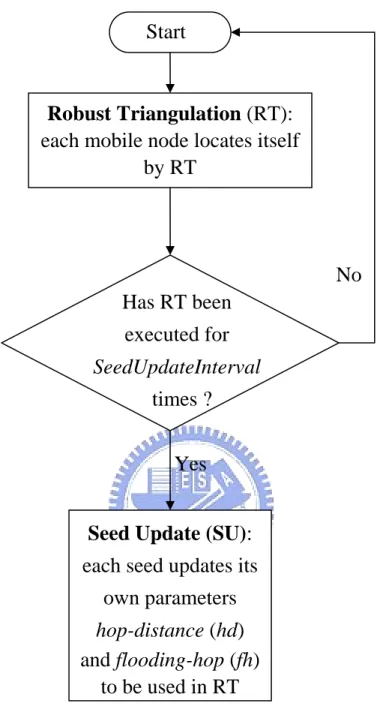
(20) Chapter 3 Proposed Dynamic Reference Localization The proposed Dynamic Reference Localization (DRL) mainly consists of two phases: 1.. Robust triangulation: Every mobile node can locate itself by triangulation with reference information it obtains.. 2.. Seeds update: Each of the seeds has its own parameters used to provide information for localization of other nodes. The parameters have to be dynamically updated according to the current surrounding conditions of a seed, such as node density.. Figure 1 shows the flowchart of DRL that includes two processes: Robust. Triangulation and Seed Update. And their detail flowcharts are shown as Figure 2. Robust triangulation.Figure 2 and Figure 3, respectively. Figure 2shows how a mobile node locates itself with information it obtains, and Figure 4 shows how this information exploited between seeds and mobile nodes. Figure 3 shows how each seed updates it parameters.. 18.

(21) Start. Robust Triangulation (RT): each mobile node locates itself by RT. No Has RT been executed for SeedUpdateInterval times ? Yes Seed Update (SU): each seed updates its own parameters hop-distance (hd) and flooding-hop (fh) to be used in RT. Figure 1. Flowchart of DRL. Robust Triangulation (RT) and Seed Update (SU) would be invoked periodically. After RT has been invoked for SeedUpdateInterval times, then SU is invoked once. SeedUpdateInterval is a given constant.. 19.

(22) nodej receive p packets from different seeds. Is p = 3 ?. Yes. Regular Triangulation (see Figure 5). No. Is p = 2 ?. Yes. Triangulation by 2 seed circles & a velocity circle (see Figure 6). No. Is p = 1 ?. Yes. Triangulation by predicted position, a seed circle, and a velocity circle (see Figure 7). No. Is p = 0 ?. Yes. Intelligent backup: nodej ask its neighbor nodes for seeds information (see Figure 8). Figure 2. Robust triangulation.. 20.

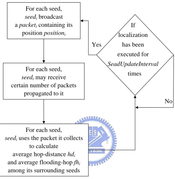
(23) For each seed, seedi broadcast a packeti containing its position positioni. If localization has been. Yes. executed for SeadUpdateInterval. For each seed, seedi may receive certain number of packets propagated to it. times. No. For each seed, seedi uses the packet it collects to calculate average hop-distance hdi and average flooding-hop fhi among its surrounding seeds Figure 3. Seed update.. 21.

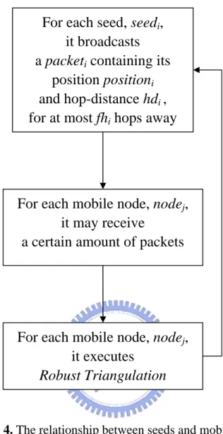
(24) For each seed, seedi, it broadcasts a packeti containing its position positioni and hop-distance hdi , for at most fhi hops away. For each mobile node, nodej, it may receive a certain amount of packets. For each mobile node, nodej, it executes Robust Triangulation. Figure 4. The relationship between seeds and mobile nodes.. 22.

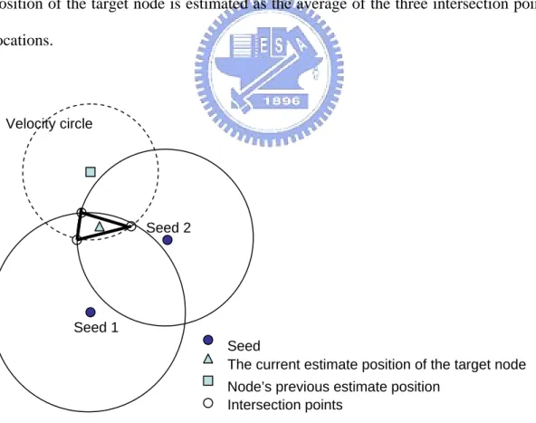
(25) 3.1 Robust triangulation For a mobile node to locate itself by triangulation, it has to get the location information of three reference nodes, usually seeds. However, it is not always that a node can get enough seeds information, especially when DRL limits the seed flooding scope to reduce network load. Therefore, when a mobile node tries to locate itself, according to the number of seeds it gets, there are four cases, as described in the following: (1) Three seeds case: If the location information of three seeds is received, we can simply do triangulation to locate the target node. Triangulation is illustrated in Figure 5. (2) Two seeds case: As illustrated in Figure 6, we can do triangulation with two seed circles and a. velocity circle. A velocity circle is a circle, whose center is the previous estimated position of the target mobile node and its radius is the maximum distance a node can move in a time unit (i.e. max velocity that a mobile node can achieve, which is a given constant). In this way, the mobile node’s current position should fall in the velocity circle. Therefore, we can estimate the mobile node’s position by triangulation with the two seed circles and the velocity circle. (3) One seed case: As illustrated in Figure 7, we have two kinds of reference information. One is that the position of the target mobile node should fall in the intersection area of the seed circle and velocity circle. And the other is that we can track the mobile node’s earlier estimate position to derive a current predicted position. Therefore, we can estimate the position of the mobile node as the average of the information 23.

(26) mentioned above, by averaging “the center of the intersection area” and “the current predicted position”. The former can be estimated as the average of the two intersection points by the seed circle and velocity circle. And the latter can be derived by the most recent two estimate positions, supposing the mobile node is moving straight with the same speed, as illustrated on the dotted arrow in Figure 7. As to the situation of the mobile node changing its moving direction, which may cause the tracking incorrect, we can prevent such an error by examining whether the current predicted position falls in the circles intersection area. If not, we just eliminate this reference information. That is, we estimate the mobile node’s position as the center of the intersection area. (4) No seed case: In this case, we propose a solution called intelligent backup. As illustrated in Figure 8, the flooding of each seed would cover a certain area. However, there may be some nodes not covered by any seeds (i.e. the nodes collect no seed information). Such nodes can ask their neighbors that have already covered by seed flooding, to pass seed information to them. If these neighbors are not covered by any seeds, they simply ask their next neighbors for help in the same way. Therefore, the inquiry will continue, until it finds a node with seed information.. 24.

(27) Seed 3. Seed 2. Seed 1 Seed The current estimate position of the target node Intersection points. Figure 5. Three seeds case: By normal triangulation with three seed circles. The position of the target node is estimated as the average of the three intersection points locations.. Velocity circle. Seed 2. Seed 1 Seed The current estimate position of the target node Node’s previous estimate position Intersection points. Figure 6. Two seeds case: By two seed circles and a velocity circle. The position of the target node is estimated as the average of the three intersection points locations.. 25.

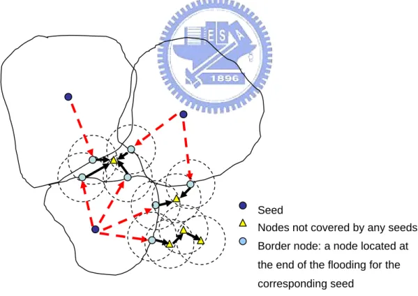
(28) Velocity circle. Seed 1 Seed The current estimate position of the target node Node’s previous estimate positions Intersection points Target node’s current predicted position. Figure 7. One seed case: By a seed circle, a velocity circle, and a current predicted position. We can estimate the node’s position, shown as a triangle in this figure.. Seed Nodes not covered by any seeds Border node: a node located at the end of the flooding for the corresponding seed. Figure 8. No seed case: By Intelligent Backup, the nodes collecting no seed information can ask their neighbor nodes for help of seed information. In this way, border nodes can propagate seeds information to these nodes. The arrows show the paths that seeds information is finally received by a node. 26.

(29) 3.2 Seeds update Seed nodes are GPS-enabled mobile nodes that can offer location information needed by other mobile nodes. Unlike DV-hop, instead of assuming all seeds having the same values of hd and fh, each seed in DRL has its own values of hd and fh, so as to reflect the current conditions around the seed. In this way, the accuracy of localization can be improved. Because all nodes, including seeds, are mobile, DRL also have to update seeds dynamically to maintain its location correctness. Especially in an irregular node distributed area, such dynamic seed information is beneficial to accuracy.. 3.2.1 Dynamic parameters of a seed In DRL, there are two special parameters in a seed, hop-distance (hd) and. flooding-hop (fh). In the process of localization, a seed broadcasts its position and hd value. hd is used to calculate the distance between a node and the corresponding seed (i.e. distance = hop-distance x hop-count). And fd is the upper bound of the hop count that a seed floods out its information. First, an information packet is broadcasted by a seed. When the packet passes a hop, it decrements its flooding-hop (fh) by 1. Once the. fh becomes 0, the packet propagation stops. In this way, we can limit the flooding area. Also, both hd and fh of a seed are dynamically updated to reflect the current conditions. If the surrounding node density is high, fh can be reduced since there is no lack of nodes for propagation. If the surrounding node density is low, hd can be increased to reflect the situation that nodes are far apart. The process of seeds updating is independent of robust triangulation, and it should be executed less frequent than the localization phase, in order not to increase. 27.

(30) network load. This is reasonable because hd and fh are related to the current node density, and the node density would not change greatly in a short time.. 3.2.1.1 Hop-distance If we neglect the difference, such as node density among local regions, we can treat hop-distance as a constant. Amorphous [1] proposed a formula for it as follows.. d hop = r (1 + e. − n local. 1 −. −∫ e. n local. (arccos t − t 1− t 2 ). π. −1. dt ). To reflect the difference among local regions, in DRL, the hop distances from different seeds may be different. Figure 9 shows the hop count between two nodes. The hop count between seed A and seed B is 7, and hd = (Euclidean distance from A to B) / 7. However, a seed may have more than one surrounding seed, so we have to do the average, as follows:. hdi =. ∑ (X. − X j ) + (Yi − Y j ) 2. i. ∑ h (i , j ). 2. , ∀j, i ≠ j. hdi is the average hop-distance between a seed i and its surrounding seeds. Here i = 1…the number of all seeds. Let seedi be the ith seed, and (Xi, Yi) is its coordinate position. The set of seedj is the seeds from which seedi receives propagated seed information for update. h(i, j) is the hop count between seedi and seedj.. 28.

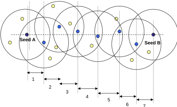
(31) Seed A. Seed B. 1 2 3 4. 5 6. 7. Figure 9. Hop count between two seeds. In this figure, between seed A and seed B,. there needs 7 hops between them. (i.e. the hop count of the shortest route between A and B is 7.). 3.2.1.2 Flooding-hop In Figure 9, for the flooding from seed A and seed B, respectively, to cover all nodes, we need to set the hop count that seed A needs to flood is 4 and B’s is 3. The flooding of seed A is shown in Figure 10. For complete coverage, we can set the flooding-hop of seed B is 4, too. In other words, the flooding-hop should be a half of the hop count between A and B. In this way, a seed knows how many hops that is sufficient for flooding coverage, instead of flooding to the whole networks. Thus, the overhead of flooding can be reduced. However, a seed may have more than one surrounding seed. So we have to do the average, as follows:. 29.

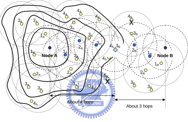
(32) fhi =. ⎡ h (i , j ) ⎤ 2 ⎥⎥ , ∀j , i ≠ j ns. ∑ ⎢⎢. fh is the average flooding-hop number between a seed and its surrounding seeds. Here ns is the number of seedi’s surrounding seeds (i. e. the set of seedj).. 4A. 4A 3A. 4A. 2A. 4B. x. 3A. 1A. Node A. 3B. 3A. 1A. 3A. 2A. 1A. 2A. 4A ,3B. 2B. 1B. 4A. Node B 1B. 2A 3A. 3A 4A. 2A. 2B. 5A 3A. x. 4A. 3B. 3B. About 4 hops About 3 hops. Figure 10. Seed flooding for mobile nodes localization. Here it illustrates a flooding. from seed A, and its flooding-hop is 4. Therefore the nodes within 4 hops away would be covered by the flooding. And, for example, there is a node marked ‘5A X’ can not be covered because it is 5 hops away from seed A. For this kind of nodes, it will be handled by the Intelligent Backup.. 30.

(33) Chapter 4 Evaluation We have evaluated the location accuracy of DRL in terms o node sped, node density and seed density by comparing that of MCL [8]. We used Java JDK1.5 [21] to develop a purpose-built simulator.. 4.1 Mobility model We assume both seeds and other mobile nodes have the same moving behavior, which we adopted the random waypoint model [10] with proper adjustment to avoid the problems discussed in [11] that average node speed would consistently decrease over time in original random waypoint model. Therefore, we set a non-zero minimum speed of nodes, according to the solution suggested in [11].. 4.2 Simulation parameters Table 1 lists the parameters related to the localization process [8]. In the. simulation, sensor nodes are randomly placed in a rectangular area of 500 m x 500 m. All nodes including seed nodes have a transmission range r of 50m. The node density is the average number of nodes in one hop transmission range [8], and the seed density is the average number of seeds in one hop transmission range [8]. We represent the velocity by a fraction of the radio transmission range (r). For example, v = 0.2r means that the node moves a distance of 0.2r, in a time unit. Assume that the maximum speed of nodes is vmax, and the minimum speed of nodes is vmin. The. 31.

(34) velocity of each node will be randomly chosen in vmin ~ vmax. We represent location estimate error by a fraction of the radio transmission range (r), too. For example, the location estimate error = 0.5r means that the distance between the estimate position and actual position is 0.5r. We express location accuracy in terms of location estimate error. To compare with the MCL approach [8], the default values of simulation parameters are set to be the same with MCL’s, and we evaluate DRL under different combination of parameters values. For the formula of nd, N is the number of nodes per m2, and πr 2 is the circle A. area a node would cover. Therefore, N π r 2 is the average number of nodes within A. the coverage circle (in other words, one hop transmission range) of one node. And sd is derived in the same way. The simulation results are the average of 10 executions, and the deployment of nodes and seeds in each execution are randomly generated.. Attributes. Value. Area size (A). 500 m x 500 m. Radio transmission range (r). 50 m. Number of nodes (N). 320 (default, for nd = 10). Number of seeds (S). ( 1, N ). Node density (nd). N 2 πr A. Seed density (sd). S 2 πr A Table 1. Simualtion parameters.. 32. Default N/10.

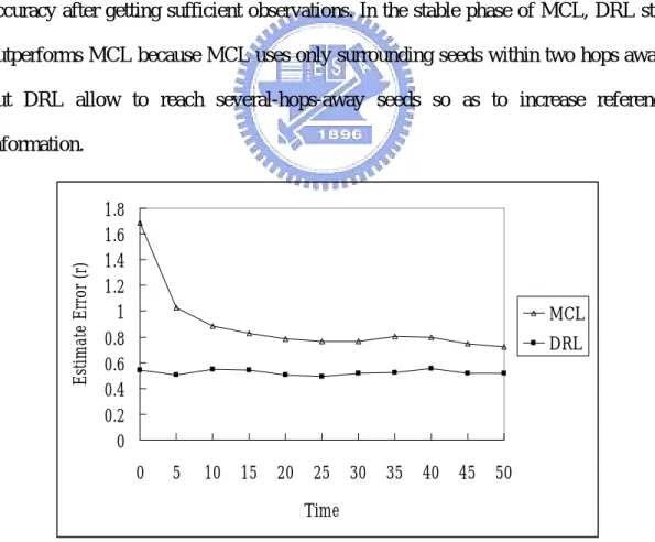
(35) 4.3 Location accuracy We compare DRL with MCL in terms of estimate error, shown as shown Figure 11. We set number of nodes N = 320 and number of seeds S = 32 so that nd = 10, sd = 0.1, which are the same parameter values used in MCL. We can see that DRL keeps location accuracy between 0.5r ~ 0.6r. MCL initially has large estimation error (initial phase), and converge later (stable phase). In overall, DRL is 26% more accurate than MCL in localization. In the initial phase of MCL, DRL outperforms MCL because DRL adopts triangulation which has good location accuracy in general, but MCL relies on new observations from seeds for prediction or filtering and can achieve reasonable accuracy after getting sufficient observations. In the stable phase of MCL, DRL still outperforms MCL because MCL uses only surrounding seeds within two hops away, but DRL allow to reach several-hops-away seeds so as to increase reference. Estimate Error (r). information. 1.8 1.6 1.4 1.2 1 0.8 0.6 0.4 0.2 0. MCL DRL. 0. 5. 10. 15. 20. 25. 30. 35. 40. 45. 50. Time. Figure 11. Location accuracy comparison. nd = 10, sd = 0.1, vmax = smax =r.. 33.

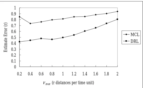
(36) 4.4 Node speed We evaluate the impact to location accuracy under different node speed settings, as shown in Figure 12. The node speed for all of the seeds and other mobile nodes are all chosen randomly in the range of (vmin, vmax], and we increase vmax by 0.2 from 0.2 to 2.0 in each iteration. Under any node speed setting, DRL still outperforms MCL. Figure 12 shows that DRL performs well when the maximum node speed is not higher than r and thus it implies that DRL is suitable for environments where node speed is under r. Also we can discover that for both DRL and MCL, the estimate error. Estimate Error (r). increases as the node speed increases. However, DRL still performs better than MCL.. 1 0.9 0.8 0.7 0.6 0.5 0.4 0.3 0.2 0.1 0. MCL DRL. 0.2. 0.4. 0.6. 0.8. 1. 1.2. 1.4. 1.6. 1.8. 2. v max (r distances per time unit). Figure 12. Impact of node speed. nd = 10, sd = 1, smax = vmax.. 4.5 Seed density We evaluate DRL and MCL for the impact of seed density to location accuracy, as shown in Figure 13. We evaluate DRL and MCL under different seed density 34.

(37) settings, and we increase seed density by 0.2 from 0.2 to 2.0 at each time interval. And we set node density = 10, node speed = r. We can see that DRL allows low seed density and has good location accuracy. For both DRL and MCL, accuracy increases as seed density grows, and DRL outperforms MCL greatly for seed density ≦ 0.08. It has also shown that DRL performs well under any seed density but MCL needs seed density higher than 0.1. Otherwise, the location accuracy is quite low. This is because that in DRL the seeds’ information flooding can achieve sufficient coverage by dynamically adjusting the number of hops in flooding it allows. In this way, a node can collect enough seeds information for localization. In MCL, the seeds that a node can refer to must be within two-hop away. Therefore, under low seed density, MCL would result in many nodes localization failures because there is no any seed for filtering. We conclude that, DRL is robust under the impact of seed density, because DRL can dynamically adjust the scope of seed information flooding. In the view of reducing communication cost, the amount of flooding should be low, while in the view of coverage to support triangulation, the amount of flooding should be high enough. When seed density is high, DRL would reduce the flooding amount and reduce communication cost. When seed density is low, DRL would raise flooding amount and has more communication cost. Therefore, when a sensor network is of low seed density, DRL performs much better than MCL.. 35.

(38) 4. Estimate Error (r). 3.5 3 2.5. MCL. 2. DRL. 1.5 1 0.5 0 0.2 0.4 0.6 0.8. 1. 1.2 1.4 1.6 1.8. 2. Seed Density. Figure 13. Impact of seed density. nd = 10, vmax = smax =r.. 4.6 Node density We evaluate DRL for the impact of node density to location accuracy. We evaluate DRL under three different node density of N = 300, N = 200, and N = 100, respectively. And we set other parameters constant with seed density of 1.0, maximum node (seed) speed of node of r. We can see that location accuracy would increase as number of nodes grows.. 36.

(39) 1.8. Estimate Error (r). 1.6 1.4. MCL(nd=10). 1.2 1. nd=4. 0.8. nd=8. 0.6. nd=10. 0.4 0.2 0 0. 5. 10. 15. 20. 25. 30. 35. 40. 45. 50. Time. Figure 14. Impact of node density. vmax = smax =r.. 37.

(40) 4.7 Comparison with other mobile localization approaches Table 2 compares DRL with other mobile localization approaches in terms of basic idea, advantages, and shortcomings. [12] is a typical range-based approach, [8] is a related work to DRL, and [9] is a tracking approach in WSN. Approach Geoorganization [12] (range based). MCL [8] (range free). Tracking [9]. DRL (proposed). Basic idea Use local information of range measurements between nodes to build a network coordinate system Use prediction and filtering — Prediction: the next possible position should fall in the circle of radius = node speed Filtering: a node filters the impossible locations based on new observations A large majority of sensor nodes with certain amount of location information are used to trace a moving target node Use DV-hop locally by using only nearby seeds. Advantages Organize a unique coordinate system by self-organization without centralized knowledge about the network topology 1. Make mobility improve localization 2. Does not need additional devices for distance measurement 3. Allow all nodes and seed to move freely. Shortcomings 1. Need large computation and message exchange 2. Need devices that support distance measurement Fail to locate a node if there is no seed within two-hop away from it. Has low power consumption because sensor nodes not related to the target can turn to sleep. Needs many pre-deployed and position-known fixed sensor nodes. 1. Reduce the amount of reference information flooding 2. Does not need additional devices as MCL 3. Allow all nodes and seed move freely as MCL. If the number of seeds is few but that of mobile nodes is large, the cost of communication would be high for Intelligent Backup. Table 2. Comparison of different localization approaches. 38.

(41) Chapter 5 Conclusions 5.1 Conclusion remarks We have presented an efficient localization scheme for mobile WSNs, called DRL, that can dynamically update reference information for cost-efficiency, and has feasible solution for nodes with insufficient seeds information. Simulation results have shown that the performance of DRL is quiet steady in location accuracy, under the variance of node speed, seed density, and node density. DRL also allows mobile nodes moving freely, and it does not need any special hardware for signal strength measurement, ultra-sound ranging, or directional antennas. We’ve shown that DRL outperforms MCL by 26%, which is an approach with the same hardware and mobility assumptions for mobile WSNs in the literature. With mobile positioning and the need for a few GSP-installed seeds, DRL is suitable for applications, such as navigation systems using e-map and community health-care systems, in outdoor environments.. 5.2 Future work In DRL, if the number of seeds is few but that of mobile nodes is large, the cost of communications may be high. This is because the intelligent backup is less efficient than normal seed flooding. If seed flooding can not reach far enough, many un-located mobile nodes need to do intelligent backup, and it would result in high communication cost. This issue deserves for further study. 39.

(42) References [1] R. Nagpal, “Organizing a global coordinate system from local information on an amorphous computer,” A.I. Memo 1666, MIT, August 1999. [2] D. Niculescu and B. Nath, “DV based positioning in ad hoc networks,” in Kluwer Journal of Telecommunication Systems, 2003, pp.267 - 280. [3] A. Savvides, C. Han, and M. B. Strivastava, “Dynamic fine-grained localization in ad-hoc networks of sensors,” MOBICOM, 2001, pp. 166 - 179. [4] C. Savarese, J. Beutel and J.M. Rabaey, “Locationing in distributed ad-hoc wireless sensor networks,” In Proc. of 2001 IEEE Int'l Conf. Acoustics, Speech and Signal Processing (ICASSP 2001), vol. 4. IEEE, Piscataway, NJ, May 2001, pp. 2037 - 2040. [5] T. He, C. Huang, B. M. Blum,J. A. Stankovic, and T. F. Abdelzaher. “Range-free localization schemes in large scale sensor Networks,” MobiCom 2003, pp. 81 - 95. [6] C. Savarese, J. Rabay, K. Langendoen, “Robust positioning algorithms for distributed ad-hoc wireless sensor networks,” In USENIX Technical Annual Conference, June 2002, pp. 317 - 327. [7] N. Priyantha, H. Balakrishnan, E. Demaine, and S. Teller, “Anchor-free distributed localization in sensor networks,” in Proc. of the First International Conference on Embedded Networked Sensor Systems, 2003, pp. 340-341. [8] Lingxuan Hu and David Evans, “Localization for mobile sensor networks,” in Proc. of the Tenth Annual International Conference on Mobile Computing and Networking (MobiCom 2004), pp. 45 - 47.. 40.

(43) [9] H. Yang, and B. Sikdar, “A protocol for tracking mobile targets using sensor networks,” in Proc. of the First IEEE International Workshop, May 2003, pp. 71 81. [10] Tracy Camp, Jeff Boleng and Vanessa Davies, “A survey of mobility models for ad hoc networks research,” Wireless Communications and Mobile Computing, Volume 2, No. 5. 2002, pp. 483 - 502. [11] J. Yoon, M. Liu; B. Noble, “Random waypoint considered harmful,” in Proc. Of IEEE INFOCOM, Volume 2, April 2003, pp. 1312 - 1321. [12] S. Capkun, M. Hamdi, J. P. Hubaux, “GPS-free Positioning in mobile ad-hoc networks,” In Proc. of HICSS, Hawaii, Jan. 2001, pp. 9008. [13] David Moore, John Leonard, Daniela Rus, and Seth Teller, “Robust distributed network localization with noisy range measurements,” in Proc. of the Second ACM Conference on Embedded Networked Sensor Systems (SenSys '04), Nov. 2004, pp. 50–61. [14] R. Iyengar and B. Sikdar, “Scalable and distributed GPS free positioning for sensor networks,” IEEE International Conference on Communications, Volume: 1, 2003, pp. 338 - 342. [15] N. Noury, G. Virone, T. Creuzet, "The Health integrated smart home information system (HIS2): rules based system for the localization of a human," in Proc. Of the 2nd Annual International IEEE-EMB Special Topic Conference, May 2002, pp. 318 - 321. [16] K.C. Wang, “Dynamic localization in wireless sensor networks,” Subproject of “Key Technologies for Wireless Sensor Networks and Their Applications in Community Health Care,” NSC, ROC, 2003.. 41.

(44) [17] N. Bulusu, J. Heidemann, D. Estrin, “GPS-less low-cost outdoor localization for very small devices,” IEEE Personal Communications, vol. 7, issue: 5, Oct. 2000, pp. 28 - 34. [18] B. H. Wellenhoff, H. Lichtenegger and J. Collins, Global Positions System: Theory and Practice, Fourth Edition. Springer Verlag, 1997. [19] D. Niculescu and B. Nath, “Ad hoc positioning system (APS) using AoA,” in Proc. of INFOCOM, San Francisco, CA, 2003, pp. 1734 - 1743. [20] P. Bahl and V. N. Padmanabhan, “Radar: An in-building RF-based user location and tracking system,” in Proc. of the IEEE INFOCOM, vol. 2, Mar. 2000, pp. 775 - 784. [21] Official site of Java standard development toolkit http://java.sun.com. 42.

(45)