An Empirical Analysis of the Price Behavior of Taiwanese Stock Warrants

1

An Empirical Analysis of the Price Behavior of Taiwanese Stock Warrants

Lee, Tsun-siou# and Jian Mei-yun*

Department of Finance, National Taiwan University Preliminary Draft

August 30, 2001

Abstract

Taiwanese stock warrants have been traded well above their theoretical prices since their inception in 1997. Instead of trying to provide explanations for the overpricing phenomenon, we investigate the behavior of the magnitude of overpricing over time. Through AR model, we first find significantly negative relationship between the magnitude of market overpricing and the returns of the underlying shares. However, the negative relationship vanishes when all end -of-month data are discarded and the usual factors such as the time-to-expiration, moneyness and liquidity are controlled. Month-end buying activities may have been created mostly by the warrant-issuing securities firms for the fear of reporting too much unrealized loss on their warrant positions, especially in the market downturns. Alternatively, if naïve warrant investors prefer to hold their positions due to the lack of liquidity in the unfavorable market situations, the overpricing of warrants would also get more serious.

When the unexpected shocks are fitted into the AR -GARCH model, the-first-order autocorrelation of daily mispricing is clearly verified. Both GARCH and ARCH effects are detected in the variance equation in most cases. For asymmetric analysis, we find that the impacts of bad news on future volatility is greater than those of good news of the same magnitude, consistent with the previous literature. The leverage effect and volatility feedback effect, however, fail to capture the essence of warrant overpricing.

# _{Dr. Lee, who is a finance professor in National Taiwan University, also serves as a director on the board of Taiwan}

Futures Exchange.

*

The authors would like to thank Professor H. M. Wu of National Taiwan University and Professor M. T.Yu of Yuan-Ze University for their insightful comments.

Corresponding author: Tsun-siou Lee

Department of Finance, National Taiwan University No.50, Lane144, Keelung Rd. Sec.4, Taipei, Taiwan, 106 e-mail:tsunsiou@mba.ntu.edu.tw

Tel:886-2-23630231 ext.2963 Fax:886-2-23633269

I. Introduction

Taiwan Stock Exchange started to trade call warrants on stocks on September 4, 1997. Most empirical studies on warrant pricing accuracy have pointed to positive bias on the market side, no matter what types of theoretical pricing models were employed. Possible explanations cited include market inefficiency, inaccurate estimation of vital parameters, and errant dividend adjustment in addition to the usual liquidity, moneyness and time-to-expiration effects. Lee and Yang (2000) offered yet another hypothesis that the ownership structure of the outstanding warrants may deviate from perfect competition, which in turn induces positive pricing error when monopolistic power is exercised to a certain degree. Since short selling is not allowed in the warrant market, their argument was supported when Herfindahl index was used as a proxy for the monopolistic power.

It is also interesting to further investigate the behavior of the magnitude of the positive pricing error when stock price changes. Black (1976) first argued that volatility typically gets higher after the underlying stock price falls, i.e., future volatility is negatively correlated with stock return. If this is the case, and the estimated volatility fails to reflect this phenomenon, then we would observe large positive pricing error of the warrants in the down market. We call it the volatility feedback effect. Brown, Harlow and Tinic (1988), French, Schwert and Stambaugh (1987), Haugen, Talmor and Torous (1991) and Yeh and Lee (2000) have demonstrated the existence of volatility feedback effect. Leverage effect represent yet another explanation why volatility tends to become higher facing stock downturns. When stock price falls, leverage in terms of market value becomes higher, which causes higher financial risk and hence the volatility of the stock. Leverage effect leads to the well-known Constant Elasticity of Variance (CEV) model of Cox and Ross (1976).

On the other hand, Rubinstein (1985) argued that even though volatility is unstable and varies along the movement of stock price, the direction of volatility changes can go either way depending on the risk characteristics of the assets of the stock-issuing company. If the volatility varies positively with the stock price, then when stock price falls, Black and Scholes (BS) model tends to overprice calls . In this case, the overpricing of the Taiwan warrants will be smaller. From a market microstructure point of view, if naïve warrant holders are reluctant to realize the loss facing market downturns, and if short selling is restricted, then the positive price errors will be enlarged in the bear market and vice versa. Thus the magnitude of positive warrant mispricing will be negatively correlated with stock price.

Accounting treatment may also contribute to the magnitude of warrant overpricing. Warrants traded in Taiwan are issued by securities firms (so-called sponsored warrants or third-party warrants). The issuing securities firms usually play the role of market makers. They reserve a portion of the warrants for market making purposes. This reserved warrant position will carry unrealized losses when premium falls. However, current accounting treatment requires that unrealized loss be reported at the month-end unaudited financial statements. In order to minimize the loss, the market makers tend to trade up the warrant price, especially toward the month-end. This type of trading behavior may cause higher warrant overpricing in the down market.

3

overpricing may be positively or negatively related to the price of the underlying stocks. If the hypothesis of volatility feedback effect is true, and the warrant pricing models fail to use correct volatility estimates (which are higher in the down market), then the overpricing will be negatively correlated with the stock price. If the naïve investors hold their warrant positions or if the market makers try to minimize accounting losses facing market downturns, then again we will see warrant overpricing to be negatively correlated with the price of the underlying stock. Rubinstein’s (1985) arguments cannot predict the relationship between warrant mispricing and the returns of the underlying shares, unless we know the risk characteristics of the stock-issuing company.

Our empirical efforts are therefore three folds. First of all, we’d like to empirically test whether the warrant overpricing display autocorrelation. Secondly, we will try to investigate the existence of GARCH phenomenon in the conditional volatility. Finally, asymmetric impacts of stock returns on warrant mispricing will be tested. Section II discusses the factors that might affect option or warrant mispricing along with the asymmetric impacts that the volatility of the underlying shares might have on the warrant price. Section III describes our empirical data and their characteristics. Section IV sets up the empirical models followed by the empirical findings in Section V. Finally, we summarize the results in Section VI.

II. Factors affecting option mispricing and the related asymmetric impacts

Ever since the seminal model proposed by Black and Scholes (1973), there have been numerous empirical studies regarding the model’s pricing accuracy. For example, Black (1975) and Lauterbach and Schultz (1990) concluded that the Black-Scholes Model tends to overprice in-the-money calls and underprice out-of-the-money ones, even though MacBeth and Merville (1979) had opposite argument. Other studies, such as Rubinstein (1985), Merton (1976) and Hull and White (1987) have also detected so-called systematic pricing errors in Black-Scholes Model. In contrast to the fixed variance assumption in Black-Scholes Model, several researchers have observed the negative relation between the volatility of stock return and the equity price. Therefore, scholars including McBeth and Mervill (1979), Beckers (1980), Swidler and Diltz (1992), Lauterbach and Schuktz (1990), Hauser and Lauterbach (1997) suggested that the CEV Model outperform Black-Scholes Model while Ferri, Kremer and Oberhelman (1986) obtained the opposite findings.

As to the estimation of specific parameters, Lauterbach and Schultz (1990) challenged the appropriateness of risk measure for warrants due to their longer time to expire. Moreover, Latane and Rendleman (1976), Chiras and Manaster (1978) claimed that the implied volatility possesses a better prediction power for true variance, however, Choi and Shastri (1989) argued that the existence of bid-ask spread may overvalue market price, therefore the implied volatility, and hence the magnitude of mispricing.

Dividend payments are one of the factors that contribute to the option mispricing. For European options with dividend -paying underlying securities, adjusting methods suggested by Geske (1979), Whaley (1981) and Merton (1973) provided some useful solutions. But, on the contrary, dividend payment may trigger early exercise for American options and then affect pricing accuracy. Whaley (1982) and Sterk (1986) found that the mispricing of options could be

minimized when the underlying security pays only one-time dividend. Geske, Roll and Shastri (1982) also pointed out that errant dividend-adjusting approach might contribute to mispricing. And for the same reason, dilution-adjusting approach such as those proposed by Galai and Schneller (1978), Lauterbach and Schultz (1990) also provided some partial explanations for mispricing.

Tauchen and Pitts (1983), and Choi and Shastri (1989) focused on the role of trading volume in the option mispricing. Using regression models, Long and officer (1997) indicated that heavily traded call options are priced more efficiently and have lower mispricing errors than thinly traded options. However, largely increased volume might reflect the arrival of new and changing market information, which leads to inefficient pricing.

For domestic studies, both Yang (1990) and Hung (1997) adopted multi-regression method that was suggested by Hauser and Lauterbach (1997), and found that out-of-the-money and short time to expiration are the majo r reasons for mispricing. Hung (1997) also suggested that the lack of liquidity makes warrant holders unwilling to suffer inevitable loss when selling, and hence the result of biased market price. Moreover, the prohibition of short selling in the warrant market may enhance the prevailing situation. Furthermore, Lee and Yang (2000) found that the higher the Herfindahl index is, the higher degree warrant mispricing will be. This suggests that in an imperfect market, the concentration of the warrant ownership and thus the monopoly power, can causes the market price of warrants to be higher than the theoretical price.

It was first discussed by Black (1976) that volatility is typically higher after the stock market falls than rises, i.e., stock returns are negatively correlated with future volatility. Subsequently, numerous researches have focused on the return volatility of financial assets, especially the asymmetric impact of good and bad news. Brown, Harlow and Tinic (1988) demonstrated that the stock price reactions to unfavorable news tend to be larger than the reactions to favorable events, and they attributed this finding to volatility feedback. In contrast, Poterba and Summers (1986) argued that volatility feedback might be too short-lived to have a major effect on stock prices. French, Schwert and Stambaugh (1987) regressed stock returns on innovations in volatility and found negative correlations attributing to the volatility feedback. Similar result was demonstrated by Haugen, Talmor and Torous (1991).

Bollerslev, Chou and Kroner (1992), Bollerslev, Engle and Nelson (1995) and Hentschel (1995) concluded that negative shocks introduced more volatility than positive ones, and this effect shows particularly apparent influence for the largest shocks. Campell and Hentschel (1992) suggested that such phenomenon might result from the “leverage effect” and “volatility feedback effect”.

For the leverage effect, the debt-equity ratio (measured in market value terms) rises as a consequence of the drop of stock price caused by negative shocks. Hence, the increased financial risk results in higher volatility in stock returns. For the volatility feedback effect, it seems plausible that changes in volatility may have important effect on the required stock returns and thus the level of stock price. However, large pieces of good news tend to be followed by other large positive shocks which increases future expected volatility, thus in turn increases the required rate of return on the stock, dampening the positive impact. On the other hand, the increased expected volatility caused by bad news will also increase the required rate of return

5

and lower the stock price, which amplifies the impact of negative shocks.

In order to capture the asymmetric impacts that stock returns might have on warrant mispricing, the empirical model must first correct all possible pricing errors that liquidity, moneyness and time-to-expiration may induce. Section IV will deal with this problem when we model our empirical methodology.

Ⅲ. The data

In order to analyze the behavior of warrant mispricing, we collected daily data of 113 individual warrants and their underlying securities from the Taiwan Economic Journal and the websites of Taiwan Stock Exchange and Yuanta Securities, Co.. Among these warrant samples, 86 out of 113 had expired by February 15, 2001. The sample period of the other 27 warrants started from their respective first trading date and ended at February 15, 2001.

We first adopted both BS Pricing Model and CEV Pricing Model to obtain daily theoretical prices for all warrants, using historical volatility as the estimates for the true variance. For warrant i (i=1, 2, ..., 113), the daily percentage deviation is then calculated and denoted as

t i PD_, ( t i m t i T t i m t i W W W PD , , , , , , , −

= , where W_m,i,t and W_T,i,t are defined as the market price and theoretical price respectively). The sample size, mean, standard deviation, skewness, kurtosis, Lagrangian multiplier test statistic with 12-period lag [LM (12)] and Ljung-Box Q test statistic with 12-period lag [LBQ (12)] for PD_BS and PD_CEV are presented in Appendix A. Besides, the percentage of positive mispricing among all the trading days was calculated for each warrant. All warrants experienced positive mean of percentage deviation during the sample period, and this figure is nearly 50% for BS model and 46% for CEV model, enhancing the popular existence of mispricing. The average standard deviation of mispricing under CEV model is about 22%, slightly higher than the average of 19% for BS model. On average, warrant mispricing had a positive skewness under both models (0.2121 for BS model and 0.1371 for CEV model), indicating that large positive mispricings are more common than large negative ones. When daily mispricing data was classified according to the sign, quite a few warrants were found with all positive mispricing throughout the sampling period. Generally speaking, warrant price closed higher than their theoretical counterparts more than 90% of the time.

LM (q) test statistics proposed by Engle (1982) is aimed to detect the characteristic of autoregressive conditional heteroskedasticity (ARCH). In order to test the null hypothesis of no ARCH up to order q in the residuals, the sugared residuals are regressed against a constant and lagged squared residuals up to order q,

t q t q t t t e e e v e = + ₋ + 2 2₋2+ + 2₋ + 2 1 1 0 2 ... β β β β (1)

where e is the residual term of the mean equation. Similar to Yeh and Lee (2000), 12-day lag is also chosen here. In fact, with the exception of nine warrant series, LM (q) for all

12 ..., , 2 , 1 =

phenomenon.

The Ljung-Box Q-statistic at lag k is a test statistic for the null hypothesis that there is no autocorrelation up to ord er k and is computed as

∑

where γ is the j -th autocorrelation and T is the number of observations. Similarly, a j

lag of 12-order is chosen to provide autocorrelation check for white noise. The results of most warrants are significant at 1% level, except for three warrants under both models. Combination of the statistics of kurtosis, Ljung-Box Q and Lagrange Multiplier test for ARCH effect reveals that most warrnats are serially correlated, heteroskedastic and leptokurtic, which indicates the appropriateness of employing AR-GARCH model to explain the data. Warrants which are insignificant in LM (12) test and LBQ (12) test are excluded in this study.

IV. The empirical model

IV.1 The mean equation

We first examine the significance of percentage deviation between warrant market price and model price. The null hypothesis of no mispricing is rejected significantly at 1% level for all samples. Given the significant existence of mispricing, whether or not the percentage deviation of warrants is affected by underlying securities’ return is one of our major focuses. We then estimate equation (3) with an extra term b₁₃R_i+_,tR_i,t to detect the asymmetric effect of spot return, PDi,t =b10+b11PDi,t 1+b12Ri,t+b13Ri,tRi,t +e1i,t

+

− (3)

where Ri,t is the return of the underlying stock of warrant i at time t and +

t i

R, is a dummy

variable which takes the value of one if Ri,t >0, and zero otherwise.

In equation (3), if the underlying stocks experience positive return at time t , then the warrant mispricing responds by a magnitude of (b12+b13). If negative return occurs for the

underlying, however, the reaction of mispricing is only b₁₂.

When trading data is observed daily, it can be found that the performance of warrants tend to behave somewhat abnormally when it approaches the end of month, although this may not be absolutely true to all warrants. Usually, the percentage deviation of warrant price seems to maintain its previous level or even enlarges toward the month-end. It has been suspected that the abnormity comes as a result of warrant issuers’ strategy. Since the issuers have to recognize losses if the warrant they hold experience considerable drop in prices, making their month-end financial reports less attractive. Issuers then have the incentive to prevent the market prices from further declines. Based on this hypothesis, equation (4) is then estimated to exclude the possible end -of-month effect and re-examine the relationship between stock price and the warrant price.

7

For each warrant, data for the last two trading days of each month are omitted and only the remaining data is used to fit equation (4),

mPD_i,t = b₂₀+b₂₁mPD_i,t−1+b₂₂R_i,t +b₂₃R_i+_,tR_i,t +e_2i,t (4) where R_i,_t and

+ t i

R_, are defined as in equation (3) and mPD_i,_t stands for the daily data of

t i

PD, excluding the last two trading days of every month.

It is also interesting to know the influence upon warrant mispricing of unexpected return shocks from the underlying stock. For all warrants, we first regressed the return of underlying security (R_i,t) on a constant and R_i,t−1,… , R_i,t−p to obtain a proxy of unexpected shocks (ε_i,t). As to the determination of optimal lag period ( p ) in equation (5), Akaike Information Criterion (AIC) and Schwarz Criterion (SC) are employed. The result in Appendix B shows that a lag of one period is enough in most cases, with four exceptions where a 2- period lag is suitable and one case where a 3- period lag is suitable.

R_i,_t =a0 +a1R_i,_t−1+a2R_i,_t−2 +...+a_pR_i,_t−_p +ε_i,_t (5)

We then tried to fit the relations between PD_i,t and ε_i,t−1. If there is an unexpected return shock in warrant i ’s underlying security at time t−1, would it affect the magnitude of mispricing of warrant i at time t? If the answer is “ yes ”, which direction would the process take place? Moreover, is there any asymmetric effect of shocks from the stock market on the magnitude of warrant mispricing? To answer all these questions, we construct equation (6a) and introduced a dummy variable S− to distinguish stock return shocks from different directions. In equation (6a), a positive ε_i,t−1 implies that the underlying security has a positive unexpected shock in period t−1, defined as good news. c₂ represents the impact coefficient of good news upon mispricing (PD_i,t). In contrast, negative ε_i,t−1 implies a negative unexpected return shock in period t−1, defined as bad news, and the impact coefficient of bad news upon PD_i,t is

3 2 c

c + .

PD_i,t =c₀+c₁PD_i,t−1+c₂ε_i,t−1+c₃S_i−_,t−1ε_i,t−1+v_i,t (6a)

where Si−,t is a dummy variable that takes the value of one if εi,t <0, and zero otherwise.

Coefficient c1 in equation (6a) serves to detect the existence of first-order autocorrelation

of PD . A positive i c implies positive relationship between 2 εi,t−1 and PDi,t. In other words,

higher degree of mispricing is expected if positive unexpected shock in stock market is larger, and vice versa. Finally, positive c3 indicates the asymmetric situation that bad news from the

underlying introduces more influence upon mispricing than good ones.

mispricing. Among which three variables including time to expiration ( T ), moneyness ( X X S M = − ) and liquidity ( volume g outstandin volume trading daily =

L ) are considered as the most influential. Therefore, we tried to regress PD on a constant, T , M and L in equation (7) to get the residual term Wi,t. Since possible effects from these three factors have been removed, Wi,t is

then called “ modified mispricing ” (modified PD) of warrant i at time t. PDi,t =β0 +β1Ti,t +β2Mi,t+β3Li,t+Wi,t (7)

Similar to the logic of equation (6a), we then model W_i,_t (the modified PD ) as the

dependent variable in equation (6b) and all the regressive coefficients carry stars (*) for distinguishing purposes. , 1 , 1 *, * 3 1 , * 2 1 , * 1 * 0 ,t it it it it it i c cW c c S v W = + ₋ + ε ₋ + −₋ε ₋ + (6b) IV.2 Variance Equation

Engle and Ng (1993) developed a new diagnostic test that emphasized the asymmetry of volatility response to news. By testing the empirical data of the Japan stock market with several related GARCH models including GARCH model (Bollerslev, 1986), exponential GARCH (EGARCH, Nelson, 1990), asymmetric GARCH (AGARCH, Engle, 1990), nonlinear asymmetric GARCH model (NGARCH, Engle and Ng, 1993) and GJR (Glosten, Jagannathan and Runkle) GARCH model, Engle and Ng (1993) suggested that the GJR GARCH model is the best parametric model. Further, Yeh and Tsai (1996) applied the new diagnostic test to the Taiwan Stock Market with the GARCH, GJR GARCH, and EGARCH models. Their results were consistent with those of Engle and Ng (1993) and supported that the GJR GARCH model is most capable of capturing the asymmetric impact of new information on return volatility.

As suggested by Engle and Ng (1993), the GJR GARCH (1,1) model is the best ARCH family model to capture the asymmetric impacts of new information. We then extend the procedure proposed by Pagan and Schwert (1990), Engle and Ng (1993) and make some reasonable adjustments to examine the influence of unexpected shock upon volatility (the conditional variance) in the warrant market. Our conditional variance equation (8a) follows the GJR GARCH model with an extra term of 2

1 , 1 , − − − it t i v W , 3 , 1 2 1 , 1 , 2 2 1 , 1 0 , − − − − − + + + = it it it it t i d d v dW v d h h (8a)

where hi,t stands for the conditional variance of vi,t given information set available at time

1 −

t [h_i,t =Var(v_i,t I_i,t−1)] and W_i,−_t is a dummy variable which takes the value of one if vi,t <0, and zero otherwise.

In equation (8a), v_i,t−1>0 implies positive unexpected shocks of warrant i at period 1

−

9

1

d . Negative shocks, however, affect warrants’ volatility through the coefficient d1+d2 .

Positive d3 indicates the nature of time-varying volatility and volatility clustering. If hi,t is

higher due to larger vi,t−1 in absolute terms, d would be positive. Positive 1 d , on the other 2

hand, implies that bad news introduces more volatility in the warrant market than good ones. Since h_i,t is defined as the conditional variance of v_i,t derived from equation (6a), equation (8a) can be viewed as an extension of equation (6a). Similar logic can then be augmented to model equation (8b),

* 1 , * 3 2 * 1 , * 1 , * 2 2 * 1 , * 1 * 0 * , ( ) ( − ) − − − − + + + = it it it it t i d d v dW v e h h (8b) where * ,t i

h stands for the conditional variance of v given information set available at time i*,t

1 − t [h_i*_,t =Var(v_i*_,t I_i,t−1)] and * , − t i

W takes the value of one if v_i*_,t <0, and zero otherwise. Since equation (3) through (8b) have to be fitted for each individual warrant and diversities among the samples are expected, the average coefficient and test statistics proposed by Fama and MacBeth (1973) will be adopted to make inferences about the overall warrant market.

V. Model estimation and results analysis

V.1 Relations between stock return and warrant mispricing

We estimate equation (3) and (4) under AR (1) and the results are tabulated in Table 1. The results indicate that the coefficient b for all warrants is significantly positive at 1% level under 11

both BS and CEV model. This fact is also found when b₂₁ is observed. In contrast, the estimate for b and 12 b is significantly negative at 1% level in most cases. Coefficients 22 b and 13 b , 23

however, tell quite different stories. For b , only 15 and 16 samples carry significant results at 13

5% level under BS and CEV model respectively. b₁₃ is positive in most of the significant cases (13 out of 15 and 13 out of 16 respectively). Compared to b13, 26 (with 18 positive ones) and 29

(with 20 positive ones) samples are found with significant b at 5% level under BS and CEV 23

model respectively. In spite of the insignificance, both the average of b and 13 b for all 23

samples are positive, which indicates that the mispricing tends to react more to negative stock returns than positive ones.

Both b₁₁ and b₂₁ are significantly positive for most samples, which reveals that the magnitude of warrant mispricing can partially be explained by one-period-lagged mispricing. This highlights that the phenomenon of first-order autocorrelation does exist in daily mispricing in the Taiwan warrant market. The average level of b for all samples is -0.8376 and -0.8705 12

under BS and CEV model respectively. Despite the overwhelming significance at 1% level, none of them is positive, indicating that the return of underlying security (R_i,_t) has negative influence

upon warrant mispricing. In other words, positive mispricing gets more serious in down market situation.

Given the basic statistics presented in Appendix A, it is undoubted that positive mispricing is expected as the “ normal ” situation in the Taiwan warrant market till now. The combination of positive mispricing and negative b₁₂ points to an interesting story. On average, the magnitude of mispricing evaluated under BS model will be driven down 0.8376% when the underlying stock market experience 1% positive return. Thus positive returns in the underlying stock market help to narrow the mispricing in the warrant market and bring the market price closer to the theoretical price. Under down market condition, however, the percentage deviation of warrant price increases by 0.8376% for every percentage of negative return in the stock market.

In order to provide a better explanation, we try to examine the stock market performance during the sample period. The TAIEX Index on September 4, 1997 is 9147.85 and went down to 6104.24 on February 15, 2001. Despite of the rise from early 1999 to early 2000, the downward trend is quite obvious if we plot the daily index from 1997 to 2001. As a result, the warrant price performed “ relatively well ” than the underlying stock price. In other words, the warrant price appeared to show downward rigidity even when its underlying security performed badly.

Table 1

AR analysis of the effect of underlying returns upon mispricing in the warrant market

Compute the percentage deviation (PD_i,t) under both Black-Scholes Model and CEV Model. Next, estimate equations (3) and (4) under AR (1) with an extra term R_i+_,tR_i,t aimed to detect the asymmetric impact. Then, substitute mW_i,t for mPD_i,t to exclude both the end-of-month effect resulted from issuers’ support and major influencing factors (T, M, L) and estimate equation (9).

t i t i t i t i t i t i b b PD b R b R R e PD_, = ₁₀+ _{11 ,−1}+ _{12 ,} + ₁₃ +_{, ,} + _, (3) t i t i t i t i t i t i b b mPD b R b R R e mPD_, = ₂₀ + _{21 ,−1}+ _{22 ,} + ₂₃ +_{, ,} + _, (4) t i t i t i t i t i t i b b mW b R b R R e mW, = 30+ 31 , 1+ 32 , + 33 , , + , + − (9) 0 1 , , = > + t i t i if R R , Ri,t =0 if else + t i

mPD, :PDi,t after the last two trading days of each month have been excluded

Equation (3) Equation (4) Equation (9)

10 b b₁₁ b₁₂ b13 b20 b21 b22 b23 b30 b31 b32 b33 10% 31 (31)* 104 (104) 103 (0) 27 (23) 32 (32) 104 (104) 91 (1) 25 (22) 18 (8) 104 (104) 47 (16) 32 (19) 5% 25 (25) 104 (104) 102 (0) 15 (13) 26 (26) 104 (104) 89 (0) 14 (14) 12 (4) 104 (104) 38 (13) 23 (15) 1% 15 (15) 104 (104) 100 (0) 4 (4) 14 (14) 104 (104) 86 (0) 0 (0) 4 (1) 104 (104) 29 (10) 10 ( 8) Coef. 0.0084 0.9735 -0.8376 0.1085 0.0089 0.9719 -0.7294 0.0994 -0.0003 0.8809 -0.0882 0.0309 BS t 1.4361 c 79.5502 a -6.9695 a 0.5378 1.4168 c 74.1420 a -5.6365 a 0.4572 -0.0915 27.9244 a -0.6839 0.1438

13 10% 36 (36) 104 (103) 102 (0) 23 (19) 35 (35) 104 (104) 90 (1) 24 (19) 20 (8) 104 (104) 47 (14) 32 (20) 5% 32 (32) 104 (103) 100 (0) 16 (13) 25 (25) 104 (104) 88 (0) 11 (10) 11 (3) 104 (104) 40 (12) 22 (14) 1% 17 (17) 104 (103) 98 (0) 2 (2) 13 (13) 104 (104) 86 (0) 2 (2) 3 (1) 104 (104) 29 (10) 10 (7) Coef. 0.0177 0.9575 -0.8705 0.0953 0.0084 0.9714 -0.7640 0.0896 -0.0006 0.8798 -0.0964 0.0494 CEV t 3.1303 a 73.6165 a -6.3544 a 0.4173 1.3898 c 74.2809 a -5.2641 a 0.3679 -0.1501 27.4461 a -0.6588 0.2025 * Numbers in parentheses are the samples with significantly positive coefficient

a : significance at 1% level b : significance at 5% level c : significance at 10% level

Table 1 also offers the estimates for equation (4). After excluding the data of the last two trading days, the overall regression results are quite similar to those of equation (3). The most exciting finding is that b , though still negatively significant at 1% for almost every sample, ₂₂ becomes smaller (in absolute term) with an average of -0.7294 and -0.7640 under BS and CEV model respectively. After the adjustment of end-of-month effect, only 0.7294% decline in mispricing (evaluated by BS model) is expected when the underlying stock experiences 1% positive return. Compared with equation (3), positive stock return also pulls down the market price of warrants to their theoretical price, but in a lower speed. In bad condition, the percentage deviation in the warrant market widens only 0.7294% following a 1% negative return in the stock market, indicating that the warrant price seems to be less rigid.

The comparison of the estimates of equation (3) and (4) can be used to interpret the effect resulted from warrant issuers’ strategy. When the stock market is going up, the price of warrants approach down to the theoretical price. Warrant issuers’ action, if exists, helps to speed up this process and narrow down the overpricing more quickly. In the case of negative stock returns, overpricing tends to widen. Warrant issuers’ supporting action for the fear of accounting losses helps to strengthen (or even enhance) the price rigidity of warrants and enlarge the overpricing.

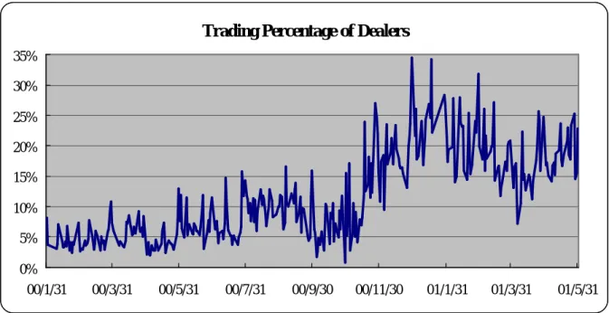
To further support our conjecture about warrant issuers’ market making activities at the month-end, we collect the data of the issuers’ trading volume for each day from January 2000 to May 2001. The issuers’ market share (defined as their trading volume divided by the total trading volume of the warrant market) for the last two trading days of each month are calculated and denoted as Ratio 2. In contrast, Ratio 1 denotes the trading share of the warrant issuers for trading days other than the last two. It’s quite clear from Table 2 that Ratio 2 is higher than Ratio 1 throughout the whole period. The U-statistic of Mann-Whitney-Wilcoxon significantly reject the null hypothesis that Ratio 2 is equal to or smaller than Ratio 1 at 5% level, indicating that the participation of dealers grows much higher at the month-end, consistent with the hypothesis of price support strategy. The cyclic trend can also be captured in Figure 1. If we further define ∆Ratio = Ratio 2－Ratio 1, the correlation coefficient ρ between ∆Ratio and Index Return is -0.27527.

15

Table 2 Ratio 1, Ratio 2, and Index Return

Figure 1 Daily Trading Percentage of Dealers

Trading Percentage of Dealers

0% 5% 10% 15% 20% 25% 30% 35% 00/1/31 00/3/31 00/5/31 00/7/31 00/9/30 00/11/30 01/1/31 01/3/31 01/5/31

Year / Month Ratio 1 Ratio 2 △Ratio Index Return

00/1 4.57% 5.60% 1.03 % 10.69% 00/2 4.07% 5.49% 1.42% 0.68% 00/3 4.63% 9.10% 4.47% 2.75% 00/4 5.75% 6.72% 0.97% -13.54% 00/5 3.77% 10.46% 6.69% 5.92% 00/6 7.04% 10.20% 3.16% -7.21% 00/7 6.71% 12.96% 6.25% 0.77% 00/8 9.82% 9.98% 0.16% -2.95% 00/9 9.41% 13.77% 4.36% -22.01% 00/10 6.41% 8.14% 1.73% -10.26% 00/11 11.99% 18.84% 6.85% -9.76% 00/12 17.58% 29.04% 11.46% -10.76% 01/1 23.37% 24.23% 0.86% 21.01% 01/2 20.02% 23.09% 3.07% -0.09% 01/3 18.83% 20.70% 1.87% 5.28% 01/4 15.85% 20.29% 4.44% -8.07% 01/5 18.53% 19.19% 0.66% -4.93% Average 11.08% 14.58% 3.50% -2.50% U-statistic U = 94 < U ( n₁ =17, n₂ =17, a ＝0.05 ) = 96 ρ = -0.27527

In addition to the end-of-month effect resulting from issuing entities’ support, it is possible that general investors’ attitude toward the warrant market also contributes to the warrant price rigidity. It has been observed that warrant investors become more reluctant to sell when the spot market gets bearish. Since considerable loss due to lack of liquidity is inevitable, they prefer to hold and wait. Consequently, the warrant price may be too weak to reflect the true value and the positive bias is then expected, especially when short selling warrants is prohibited.

Based on this hypothesis, we construct equation (9) and modeled mW_i,t as the dependent variable, where mW_i,t is the residual of equation (7) after excluding the data of the two month-end trading days, and adjusting for the biases caused by T , M and L. The results are tabulated in the third panel of Table 1.

mWi,t =b30+b31mWi,t1+b32Ri,t+b33Ri,tRi,t+e3i,t +

− (9)

After the substitution of the dependent variable mWi,t, only b remains significant 31

verifying the characteristic of first-order autocorrelation. The average of b turns to -0.0882 32

and -0.0964 under BS and CEV model respectively, much smaller (in absolute term) than b 22

and b₁₂. Moreover, only approximately 40% of the total samples carry significant b₃₂ and the average test statistics for both models are insignificant (t-statistics = -0.6839 and -0.6588 respectively).

All the estimates of equation (3), (4) and (9) illustrate consistent and interesting results. Using BS model as the example: while the original percentage deviation (PD_i,t) is significantly affected by the spot return (R_i,t) through the impact coefficient of -0.8376, this negative relation also exists after the adjustments of end -of-month effect. The impact coefficient, however, changes to -0.7294, indicating the effect of warrant issuers’ support which helps to drive down warrant price to its theoretical level when the stock market experiences positive return but strengthen the price rigidity of warrants (preventing warrant price from further declines) and enlarge the warrant overpricing in the case of negative stock return. The negative relations between mispricing and stock return finally disappear when three factors (T, M, L) are adjusted. Investors’ unwillingness to sell and to recognize losses due to lack of liquidity does result in bias ed market price and hence widen the overpricing when the spot market becomes unfavorable.

V.2 The impact of unexpected shocks on return and volatility

Equation (6a), (8a), (6b) and (8b) are estimated under AR (1) and GARCH (1,1) specifications using the algorithm developed by Berndt, Hall, Hall and Hausman (1974) and the results are tabulated in Table 3 and Table 4. For mean equation (3a) and (3b), the coefficients c 1

and c1* for all warrants are significantly positive at 1% level under both BS model and CEV

model, verifying the characteristic of autocorrelation in the Taiwan warrant market again. The signs of the estimates for c and 2 c (3

* 2

c and c ), however, appear to be quite mixed. For 3* c , 2

17

respectively. Among the samples with significant c2, only 28% (9out of 32) are positive for BS

model and 40% (16 out of 40) are positive for CEV model. The situation of c is even less *2

appealing for only 14 (with 5 positive ones) and 14 (with 4 positive ones) significant samples at 5% level under BS and CEV model respectively. The results also demonstrate the lack of evidence to support the asymmetric influence of unexpected shocks from spot market since only 18 (with 9 positive ones) and 32 (with 25 positive ones) samples with significant c₃ and 14 and 16 samples with significant c are observed. ₃*

Table 3

AR-GARCH analysis of conditional means and variances

Regress the return of underlying security (R_i,t) on a constant and suitable lagged R_i,t−p according to AIC and SC) to form the proxy of unexpected return shocks (ε ). Then, estimate _i,t equations (6a) and (8a) under AR (1) and GARCH (1,1) specifications using the algorithm developed by Berndt, Hall, Hall and Hausman (1974).

t i p t i p t i t i t i a aR a R a R R_, = ₀+ _{1 ,−1}+ _{2 ,−2} +...+ _,− +ε_, (5) Means : t i t i t i t i t i t i c c PD c c S v PD_, = ₀+ _{1 ,−1}+ ₂ε _,−1+ ₃ −_,−1ε_,−1+ _, (6a) Variance : 1 , 3 2 1 , 1 , 2 2 1 , 1 0 , − − − − − + + + = it it it it t i d d v dW v d h h (8a) ) ( _{, , 1} ,t = it it− i Var v I h 0 1 _, , = < − t i t i if S ε , S_i−_,t =0 if else 0 1 , , = < − t i t i if v W , Wi,t =0 if else −

Equation (6a) Equation (8a)

0 c c₁ c₂ c3 d0 d1 d2 d3 BS 10% 69 (68) 104 (104) 38 (12) 25 (11) 32 (32) 77 (77) 51 (32) 100 (100) 5% 59 (58) 104 (104) 32 (9) 18 (9) 25 (25) 67 (67) 46 (30) 100 (100) 1% 43 (42) 104 (104) 22 (6) 13 (7) 15 (15) 49 (49) 31 (19) 99 (99) Coef. 0.0136 0.9638 -0.0454 0.0318 0.0001 0.1826 0.0548 0.7564 t 2.5093 a 76.4225 a -0.5095 0.1968 2.2209 b 2.3966 a 0.4956 14.0705 a CEV 10% 70 (68) 104 (104) 45 (18) 36 (17) 34 (34) 83 (83) 44 (24) 100 (100) 5% 63 (62) 104 (104) 40 (16) 32 (15) 26 (26) 74 (74) 37 (21) 100 (100) 1% 45 (44) 104 (104) 30 (11) 27 (13) 11 (11) 55 (55) 25 (14) 98 (98) Coef. 0.0125 0.9625 -0.0501 0.0360 0.0002 0.2439 0.0094 0.7340 t 2.7320 a 80.7804 a -0.5385 0.2120 1.6839 b 2.6684 a 0.0753 13.0148 a * Numbers in parentheses are the samples with significantly positive coefficient

a : significance at 1% level b : significance at 5% level c : significance at 10% level

Table 4

AR-GARCH analysis of conditional means and variances

Substitute W_i,t for PD_i,t and estimate equations (6b) and (8b) under AR (1) and GARCH (1,1) specifications using the algorithm developed by Berndt, Hall, Hall and Hausman (1974).

Means : * , 1 , 1 , * 3 1 , * 2 1 , * 1 * 0 ,t it it it it it i c cW c c S v W = + ₋ + ε ₋ + −₋ε ₋ + (6b) Variance : * 1 , * 3 2 * 1 , * 1 , * 2 2 * 1 , * 1 * 0 * , ( ) ( − ) − − − − + + + = it it it it t i d d v dW v e h h (8b) ) ( *_{, , 1} * ,t = it it− i Var v I h 0 1 , , = < − t i t i if S ε , Si,t =0 if else − 0 1 *, * , = < − t i t i if v W , Wit 0 if else * , = − Equation (6b) Equation (8b) * 0 c * 1 c c*₂ c3* * 0 d * 1 d d₂* d3* BS 10% 15 (10) 104 (104) 19 (6) 20 (16) 72 (72) 66 (66) 63 (52) 93 (93) 5% 8 (6) 104 (104) 14 (5) 14 (10) 61 (61) 55 (55) 47 (39) 91 (91) 1% 7 (5) 104 (104) 8 (4) 4 (3) 40 (40) 33 (33) 25 (20) 91 (91) Coef. 0.0004 0.9057 -0.0259 0.0646 0.0002 0.1739 0.1519 0.6383 t 0.1607 33.3548 a -0.2750 0.3924 3.3318 a 2.1861 b 1.1314 8.3519 a CEV 10% 16 (13) 104 (104) 22 (6) 21(18) 69 (69) 68 (68) 52 (39) 93 (93) 5% 12 (10) 104 (104) 14 (4) 16 (14) 54 (54) 57 (57) 43 (32) 91 (91) 1% 4 (4) 104 (104) 7 (1) 6 (6) 39 (39) 35 (35) 25 (18) 91 (91) Coef. 0.0006 0.9027 -0.0380 0.0864 0.0002 0.1928 0.1287 0.6448 t 0.2240 33.3190 a -0.3618 0.4672 2.6125 a 2.3245 a 0.9286 7.6750 a * Numbers in parentheses are the samples with significantly positive coefficient

a : significance at 1% level b : significance at 5% level c : significance at 10% level

Positive c₁ and c₁* support the existence of autocorrelation for the daily mispricing in the Taiwan warrant market. For warrants with significantly negative c , mispricing widens in 2

response to bad news from the stock market and narrows down when good news hits the market. This process, however, may not be interpreted as the common phenomenon due to the insignificant average test statistic. Even fewer samples with significant c*2 indicates that the

modified mispricing (W_i,t) is less sensitive to shocks from the stock market. This interpretation is somewhat instinctively reasonable since the factor of moneyness (

X X S

M = − ) has been removed from W_i,t so that information effect of the stock price movement has been reflected. Furthermore, the suspicion of asymmetric influence upon mispricing of stock market shocks cannot be concluded thoroughly due to the diverse regression results for both c3 and

* 3

c . Taking c3 of CEV model as an example, the figures in Table 3 show that 15 (17) warrants’

19

mispricing react more to bad (good) news of their underlying than good (bad) ones while the other 72 samples do not show any asymmetry significantly. However, since the average test statistic is not significant and so minor are the significant cases that we may have difficulty to generalize the results to the whole warrant market.

Variance equation (8a) and (8b) are designed to analyze the potential influence of unexpected shocks upon conditional volatility. Notice that the coefficient d3, aimed to detect

GARCH effect, is significantly positive at 1% level in most cases under both BS and CEV model (99 and 98 samples respectively). These overwhelming results suggest the time -varying volatility and volatility clustering. For ARCH effect, 67 and 74 warrants are found to carry significantly positive d1 respectively. The relevant figures for significant

* 1

d in equation (8b) are 55 and 57 cases. Finally, the number of samples with significant d is 46 for BS model and 37 for CEV 2

model while 47 and 43 cases are found with significant d2* under two pricing models.

Positive d implies that 1 hi,t will be higher if original mispricing (PDi,t) has large vi,t−1

in absolute terms. For similar interpretation, positive d1* also shows the positive relations

between * ,t

i

h and v_i*_,t−1 in absolute terms. Despite some of insignificant cases, both the average test statistics are significant at 5% level, suggesting the warrant market is ARCH-related.

The d₂ phenomenon is positive for about 60% of the significant warrants (30 out of 46 and 21 out of 37), which may infer the existence of leverage effect and volatility feedback effect. For leverage effect, higher volatility is expected when financial risk increases as a consequence of the decline of mispricing caused by negative shocks. For volatility feedback effect, expectation of higher volatility caused by bad news would increase the required rate of return and lower the price, which amplifies the impact of negative shocks. Significantly negative cases, on the other hand, convey that when there exist good news from the warrant market itself (vi,t−1>0), warrant mispricing reacts favorably, causing volatility to rise. And it will increase consistently if investors chase after good news, which contributes to a further increase in volatility. Whether positive or negative, however, cases of significant d represent only a small 2

portion of the total samples and the average test statistics also deny the overall asymmetry in the warrant market. Since this is also true fo r d₂*, it is difficult to achieve the overall conclusion of asymmetric influence of unexpected shocks upon conditional variance.

V.3 Diagnostic test

In order to ensure that the specification of AR-GARCH model are correct, two more tests for the residual term (unexpected return shocks) of equation (6a) and (6b) are carried out. First of all, Ljung-Box Q test on autocorrelations and partial autocorrelations of the standardized residuals is used to test for remaining serial correlation in mean equation. If the mean equation is correctly specified, all Q-statistics should not be significant. Besides, Correlogram Squared Residuals that emphasize the squared standardized residuals are applied to check the specification of variance equation, particularly the remaining ARCH effect. For a correctly specified variance equation, there should be no ARCH left.

Most of the Ljung-Box (24) for residuals is insignificant, which supports the white noise nature of the residuals. Ljung- Box (18) is further computed for those exceptions and the result turns insignificant, indicating that the residuals are only autoregressive in the higher order. Correlogram Squared Residuals test statistics also suggest that there remains no ARCH effect in the squared standardized residuals for most samples. In general, both the mean equations and variance equations are quite correctly specified. In addition, the τ statistics of Dicky-Fuller test are all significantly different from zero, rejecting the null hypothesis that the time series data has unit roots.

Furthermore, diagnostic tests on the GJR GARCH model are utilized to test the capability of capturing the asymmetric impact of good and bad news upon conditional variance. For instance, equation (10) is constructed for equation (6a) and (8a),

it it it it it it t i t i v W k v W k W k k h v , 1 , 1 , 3 1 , 1 , 2 1 , 1 0 2 , , ) ( = + −₋ + −_{− −} + +_{− −} +θ (10)

The purpose of the test for coefficient k (sign bias test) is to clarify whether positive and 1

negative innovations affect future volatility of warrants differently from the model prediction. The coefficient k (2 k ) is used to test whether larger negative (positive) innovations are 3

correlated with larger biases in predicted volatility, which is called a negative (positive) size bias test. In most cases, all the sign and size bias tests together with a joint test suggest that the squared standardized residual 2

, , ) ( t i t i h v

is i.i.d., as none of the coefficients are significantly different from zero, and hence, GJR GARCH model is considered acceptable in this research.

VI. Conclusions

The warrant market of Taiwan has experienced a great positive mispricing since its inception when Black-Scholes model and CEV model are used as the benchmark. The average positive mispricing may be as high as 50%. In this study, we observed significantly negative relations between warrant mispricing and returns of the underlying securities, which implies that positive stock returns help to reduce the discrepancies between market price and theoretical price while negative returns in the stock market tend to result in more serious mispricing. The average coefficient is -0.8376 for BS model and -0.8705 for CEV model.

After the exclusion of end -of-month effect and major influencing variables (T, M, L), the impact coefficient adjusts down to only -0.0882 and -0.0964 respectively and becomes insignificant. This result reveals that warrant issuers’ supporting strategy, if exists, helps to narrow mispricing in good market but solidify the price rigidity of warrants (prevent market price from further declines) and enlarge the overpricing in bad market. Besides, warrant investors become more reluctant to sell and prefer to hold when the spot market gets less attractive since considerable loss due to lack of liquidity is inevitable.

21

market, the overall influence cannot be clearly identified due to the diverse results and the insignificant average test statistic. Only the existence of first-order autocorrelation of daily mispricing can be verified through the empirical results.

For the analysis of the influence upon conditional variance of unexpected shocks, both the GARCH and ARCH effect are proven significant in most cases. The estimates for asymmetry toward unexpected shocks from the stock market, however, tell quite different stories. Some evidences are found that conditional volatility of mispricing reacts more to bad news than to good ones under the GJR GARCH model. The leverage and volatility feedback effects supported by some significant samples, however, fail to capture the essence of the overall warrant market. Therefore, it is difficult to conclude volatility asymmetry as the common phenomenon in the warrant market. Finally, all the impact coefficients of unexpected stock returns seem to confirm the efficiency of the warrant market for no more volatility is introduced by unexpected return shocks from the underlying securities.

As a final note, if the accounting requirements induce abnormal trading behavior of the warrant issuers and the restrictio n on warrant short selling further enhance the pricing bias, especially in bearish market, then the market can never learn to function itself through market mechanism. Taiwan Futures Exchange is scheduled to launch stock index options toward the end of the year 2001. We hope all related tax and accounting treatments are well designed so that market efficiency can be achieved.

Appendix A

Basic Statistic

BS Model CEV Model

Code obs Mean S. D. Skewness Kurtosis %(1) LM (12)(2) LB (12)(3) Mean S. D. Skewness Kurtosis %(1) LM (12)(2) LB (12)(3) 0501 271 0.738 0.192 -0.225 2.309 100 215.88 a 2278.90 a 0.725 0.224 -0.538 2.513 100 210.43 a 1814.70 a 0502 271 0.672 0.201 0.559 1.706 100 187.53 a 1683.20 a 0.648 0.225 0.513 1.621 100 190.93 a 1708.80 a 0503 270 0.336 0.242 0.944 3.233 98.15 193.53 a 1608.30 a 0.222 0.307 0.846 2.787 71.85 170.46 a 1386.60 a 0504 269 0.601 0.287 0.209 1.295 100 211.05 a 1562.90 a 0.588 0.309 0.188 1.271 100 210.23 a 1496.20 a 0505 268 0.318 0.332 0.528 1.990 81.72 44.98 a 1635.30 a 0.222 0.416 0.447 1.761 59.33 43.24 a 1600.40 a 0506 267 0.239 0.148 -0.218 2.397 95.51 109.85 a 809.86 a 0.148 0.216 -0.362 2.131 63.67 130.25 a 940.70 a 0507 274 0.690 0.195 -0.280 2.145 100 110.62 a 1204.00 a 0.681 0.220 -0.417 2.150 100 132.95 a 99.43 a 0508 274 0.630 0.212 -0.248 2.272 100 211.70 a 1339.30 a 0.622 0.240 -0.351 2.212 100 193.19 a 1268.40 a 0509 267 0.353 0.167 0.135 3.049 100 112.57 a 921.43 a 0.263 0.240 -0.204 2.362 76.03 124.99 a 1126.40 a 0510 267 0.762 0.178 -0.909 3.799 100 177.65 a 1368.30 a 0.714 0.222 -0.792 3.419 100 181.24 a 1421.00 a 0511 267 0.647 0.223 0.157 1.848 100 144.56 a 1198.70 a 0.628 0.256 -0.061 1.764 100 147.30 a 1031.60 a 0512 267 0.697 0.237 -0.399 2.033 100 140.20 a 1327.30 a 0.691 0.257 -0.519 2.104 100 146.99 a 1583.30 a 0513 267 0.728 0.281 -0.797 2.200 100 126.76 a 1160.00 a 0.677 0.388 -0.958 2.456 90.26 100.84 a 1145.10 a 0514 267 0.748 0.184 0.135 1.710 100 203.23 a 1065.00 a 0.744 0.199 -0.039 1.793 100 189.78 a 982.92 a 0515 266 0.558 0.185 0.192 2.630 100 159.46 a 1312.80 a 0.544 0.207 0.238 2.315 100 159.66 a 1298.70 a 0516 266 0.232 0.109 -0.039 2.871 97.74 122.09 a 1094.60 a 0.162 0.121 0.454 2.646 95.49 110.12 a 1144.70 a 0517 264 0.161 0.131 0.105 1.385 90.91 171.77 a 919.64 a 0.120 0.160 0.179 1.425 71.21 138.83 a 743.35 a 0518 264 0.270 0.221 0.992 2.716 99.24 162.30 a 1326.70 a 0.208 0.248 0.892 2.559 83.33 172.56 a 1332.20 a 0519 264 0.145 0.076 0.658 3.419 98.48 162.50 a 1189.20 a 0.108 0.071 -0.270 5.391 94.70 167.92 a 1168.60 a 0520 402 0.298 0.074 0.035 1.602 100 201.47 a _1853.90 a _{0.281 0.071 0.371 1.851 100 192.27} a _1663.40 a 0521 264 0.096 0.098 0.711 2.403 84.85 147.00 a 932.58 a 0.043 0.064 1.040 4.472 77.65 152.21 a 737.02 a 0522 265 0.271 0.080 -2.583 8.521 97.74 148.33 a _464.08 a _{0.259 0.096 -2.538 8.148 94.34 126.96} a _446.46 a 0523 263 0.154 0.048 1.649 5.362 100 183.33 a 724.43 a 0.127 0.057 1.072 5.323 98.48 176.65 a 543.49 a 0524 265 0.156 0.041 -0.434 4.630 100 15.41 201.05 a 0.121 0.067 -0.869 3.156 92.83 33.15 a 563.96 a 0525 265 0.208 0.094 0.793 2.533 100 67.56 a 368.35 a 0.161 0.085 0.544 2.958 97.74 68.05 a 374.03 a 0526 265 0.063 0.090 1.166 4.673 72.83 207.59 a 956.37 a 0.016 0.076 -0.544 5.853 57.74 214.05 a 839.70 a 0527 265 0.251 0.098 0.511 3.063 100 145.54 a 697.07 a 0.193 0.116 0.508 3.262 95.09 139.72 a 669.20 a 0528 265 0.243 0.067 0.340 2.737 100 152.16 a _560.92 a _{0.200 0.064 0.153 2.839 100 131.41} a _523.94 a 0529 265 0.451 0.111 1.633 7.801 100 148.86 a 571.69 a 0.418 0.126 1.422 6.762 100 146.88 a 595.53 a 0530 265 0.112 0.104 1.157 5.445 89.43 157.26 a 924.16 a 0.076 0.102 1.225 4.102 78.49 144.55 a 790.29 a 0531 373 0.414 0.222 0.744 2.697 100 169.18 a 924.64 a 0.388 0.237 0.874 2.803 100 173.75 a 933.50 a 0532 267 0.553 0.226 0.774 2.491 100 125.81 a 1040.00 a 0.531 0.242 0.762 2.402 100 135.49 a 1057.30 a 0533 267 0.163 0.179 1.310 3.931 97.00 195.90 a 512.14 a 0.120 0.167 1.636 5.862 82.40 193.83 a 528.27 a 0534 266 0.119 0.161 1.373 4.317 83.08 172.73 a 758.67 a 0.074 0.150 1.857 7.048 56.02 172.72 a 748.75 a

23

BS Model CEV Model

Code obs Mean S. D. Skewness Kurtosis %(1) LM (12)(2) LB (12)(3) Mean S. D. Skewness Kurtosis %(1) LM (12)(2) LB (12)(3) 0535 266 0.430 0.289 0.779 2.260 100 171.50 a 1232.70 a 0.376 0.327 0.735 2.141 95.86 178.51 a 1294.50 a 0536 267 0.249 0.204 2.509 8.717 100 149.61 a 1410.30 a 0.216 0.218 2.490 8.509 99.25 147.45 a 1435.20 a 0537 267 0.091 0.140 1.408 5.526 80.52 197.17 a 198.87 a 0.047 0.129 1.943 8.888 50.94 193.84 a 208.38 a 0538 266 0.271 0.184 2.630 9.954 100 191.25 a 1478.10 a 0.230 0.199 2.566 9.561 99.25 191.26 a 1483.90 a 0539 266 0.208 0.228 2.491 8.545 96.99 167.79 a 1275.30 a 0.165 0.239 2.634 9.035 91.35 167.93 a 1297.20 a 0540 266 0.120 0.095 0.468 2.420 90.60 175.07 a 1402.80 a 0.088 0.079 0.397 3.793 82.71 158.14 a 1087.20 a 0541 266 0.657 0.302 -0.238 1.454 100 135.06 a 1110.60 a 0.612 0.360 -0.312 1.493 98.12 131.56 a 1182.70 a 0542 266 0.090 0.159 1.358 4.757 66.54 214.84 a 385.14 a 0.044 0.156 1.743 6.507 40.60 211.49 a 390.05 a 0543 267 0.430 0.280 1.106 2.708 100 168.43 a _1853.90 a _{0.397 0.306 1.077 2.598 100 163.32} a _1861.60 a 0544 267 0.062 0.123 3.554 22.582 71.16 238.37 a 190.12 a 0.027 0.120 4.250 29.368 37.45 238.2 0 a 184.88 a 0545 267 0.426 0.311 0.978 2.409 100 150.71 a 1515.70 a 0.379 0.341 0.994 2.355 98.88 167.54 a 1575.10 a 0546 267 0.104 0.177 2.493 10.912 75.28 226.52 a 720.96 a 0.061 0.184 2.692 11.741 46.07 225.84 a 713.13 a 0547 267 0.286 0.306 1.050 3.269 84.27 65.64 a 863.65 a 0.234 0.340 0.985 3.067 73.78 73.42 a 863.54 a 0548 267 0.271 0.288 0.939 3.291 79.78 130.16 a 548.27 a 0.236 0.314 0.909 3.100 68.16 125.28 a 541.17 a 0549 267 0.386 0.259 1.453 3.943 100 147.83 a _1299.40 a _{0.343 0.285 1.413 3.776 98.50 139.67} a _1208.70 a 0550 267 0.514 0.345 0.081 1.564 100 168.52 a 1557.50 a 0.470 0.392 0.040 1.544 87.64 175.89 a 1565.20 a 0551 267 0.420 0.276 1.125 2.839 100 132.70 a _1018.40 a _{0.390 0.303 1.103 2.698 100 117.55} a _1010.30 a 0552 267 0.794 0.193 -0.415 1.858 100 205.16 a 1461.50 a 0.778 0.223 -0.592 2.026 100 198.87 a 1367.50 a 0553 75 0.074 0.093 0.748 3.765 82.67 4.85 19.16 c 0.012 0.129 0.327 2.788 54.67 13.75 22.81 b 0554 267 0.714 0.240 -0.282 1.945 100 152.10 a 1003.30 a 0.695 0.271 -0.354 1.913 100 156.54 a 1119.20 a 0555 267 0.799 0.211 -0.761 2.337 100 132.96 a 954.62 a 0.784 0.239 -0.828 2.439 100 132.11 a 1010.10 a 0556 267 0.417 0.351 0.667 1.978 97.38 195.58 a 917.78 a 0.356 0.386 0.751 1.998 82.40 197.07 a 945.11 a 0557 266 0.394 0.312 0.921 2.314 100 156.02 a 1245.40 a 0.365 0.349 0.846 2.108 97.37 155.56 a 1176.70 a 0558 270 0.297 0.159 1.594 6.633 98.89 163.99 a 397.99 a 0.240 0.182 1.741 6.264 98.52 162.98 a 445.89 a 0559 24 0.439 0.146 -1.507 4.938 95.83 7.94 0.381 0.139 -1.188 4.199 95.83 6.88 0560 270 0.674 0.199 0.189 2.190 100 157.43 a 929.89 a 0.646 0.231 0.039 2.317 100 134.64 a 820.48 a 0561 269 0.616 0.256 0.505 1.686 100 130.44 a 1140.10 a 0.590 0.289 0.378 1.594 100 164.25 a 1329.20 a 0562 269 0.624 0.195 0.163 2.551 100 213.28 a 1802.40 a 0.601 0.228 -0.039 2.636 100 202.78 a 1728.80 a 0563 269 0.967 0.039 -1.039 3.031 100 174.77 a 1068.40 a 0.978 0.031 -1.552 4.365 100 199.12 a 1065.20 a 0564 269 0.836 0.202 -0.987 2.629 100 197.57 a 2094.60 a 0.817 0.243 -1.118 2.869 100 190.17 a 1918.90 a 0565 269 0.453 0.298 0.718 2.097 100 140.89 a 1523.50 a 0.404 0.353 0.637 1.852 95.91 115.59 a 1247.50 a 0566 268 0.543 0.354 0.125 1.527 100 212.16 a 1461.20 a 0.469 0.414 0.170 1.486 83.21 227.56 a 1650.80 a 0567 268 0.716 0.229 -0.387 2.292 100 181.91 a 1378.60 a 0.696 0.262 -0.335 2.034 100 156.05 a 1217.70 a 0568 267 0.657 0.261 0.060 1.741 100 93.55 a 753.26 a 0.605 0.310 0.045 1.674 100 105.98 a 803.45 a 0569 267 0.771 0.232 -0.521 1.967 100 161.60 a 1855.00 a 0.755 0.274 -0.699 2.183 100 166.38 a 1801.70 a 0570 267 0.886 0.123 -1.141 3.629 100 164.76 a 1540.50 a 0.887 0.136 -1.361 4.157 100 161.00 a 1554.30 a 0571 266 0.777 0.184 -0.156 1.732 100 185.69 a 1094.50 a 0.764 0.208 -0.229 1.663 100 188.34 a 1270.50 a

BS Model CEV Model

Code obs Mean S. D. Skewness Kurtosis %(1) LM (12)(2) LB (12)(3) Mean S. D. Skewness Kurtosis %(1) LM (12)(2) LB (12)(3) 0572 265 0.769 0.180 0.121 1.489 100 165.76 a 1465.50 a 0.765 0.202 -0.123 1.582 100 190.71 a 1591.30 a 0573 265 0.473 0.303 0.642 1.930 100 150.31 a 1251.70 a 0.423 0.362 0.540 1.694 95.85 123.95 a 865.87 a 0574 265 0.674 0.203 -0.072 2.118 100 191.58 a 651.97 a 0.643 0.237 -0.121 2.177 100 192.12 a 595.15 a 0575 265 0.903 0.121 -1.337 3.956 100 97.80 a 1078.60 a 0.899 0.143 -1.573 4.611 100 112.87 a 1185.40 a 0576 264 0.761 0.191 -0.011 1.614 100 187.02 a 1538.30 a 0.741 0.222 -0.172 1.653 100 193.75 a 1595.20 a 0577 262 0.316 0.287 0.716 2.077 95.42 89.89 a 478.85 a 0.232 0.354 0.672 1.936 59.16 78.68 a 467.13 a 0578 262 0.435 0.313 0.687 2.038 99.24 118.31 a 1470.10 a 0.384 0.372 0.593 1.796 91.22 99.02 a 1068.10 a 0579 267 0.456 0.231 0.727 3.241 98.13 160.34 a 834.37 a 0.441 0.259 0.595 2.711 97.75 140.27 a 780.09 a 0580 267 0.912 0.085 -0.351 1.759 100 162.79 a 1175.80 a 0.924 0.081 -0.732 2.404 100 94.24 a 854.71 a 0581 267 0.924 0.119 -1.580 4.275 100 132.68 a 1431.20 a 0.922 0.138 -1.817 5.144 100 116.12 a 1223.00 a 0582 267 0.835 0.154 -0.377 1.811 100 197.22 a 1539.60 a 0.824 0.178 -0.553 1.961 100 187.45 a 1459.40 a 0583 267 0.773 0.227 -0.430 1.714 100 195.58 a 1769.00 a 0.756 0.271 -0.611 1.893 100 191.51 a 1750.00 a 0584 267 0.638 0.276 0.005 1.509 100 195.64 a 1238.90 a 0.573 0.357 0.006