運用支撐向量機技術之FHMA/MFSK 訊號偵測

國 立 交 通 大 學

電信工程學系

碩 士 論 文

運用支撐向量機技術之 FHMA/MFSK 訊號偵測

Detection of FHMA/MFSK Signals

Based on SVM Techniques

研究生：劉人仰

指導教授：蘇育德 教授

運用支撐向量機技術之

FHMA/MFSK 訊號偵測

研究生：劉人仰 指導教授：蘇育德 博士

國立交通大學電信工程研究所

中文摘要

本 論 文 提 供 一 個 初 步 用 來 設 計 智 慧 型 通 訊 處 理 器

(intelligent

communication processor)的整合架構。智慧型通訊處理器的一個重要

特 性 是 其 可 以 利 用 離 線 式

(off-line) 的 訓 練 時 期 所 獲 得 的 知 識

(knowledge)來做及時性的訊號偵測。雖然離線式的訓練可能需要大量

的運算，但所獲得的資訊卻是很簡潔的，因此智慧型通訊處理器只需要

小量的運算就可以做訊號偵測。利用這樣的概念，我們從機械學習的觀

點來探討在多重存取環境中跳頻(frequency hopping)訊號偵測的問題。

相對於直接序列展頻(DS-CDMA)技術，跳頻技術是另一種吸引人

的多重存取技術。

除了通道統計特性，跳頻多重存取系統的效能會由兩項主要考量所

決定：波形(waveform)的設計和接收機的架構。在給定跳頻波形，我們

仍然很難設計最大相似性(ML)接收機，其主要原因是我們對於通道統

計特性的瞭解是不完整的，即使是完整的，通常相對應的條件機率分佈

(conditional pdf)是沒有簡潔的表示式。

藉由把接收到的訊號視為一個時間─頻率的圖形，我們可以把多使

用者偵測的問題轉換成圖形辨識的問題，然後運用支撐向量機的技術來

解 決 所 對 應 產 生 的 圖 形 辨 識 問 題 。 利 用 適 當 的 核 心 函 數

(kernel

function)，支撐向量機技術把收到的訊號轉換到高維度的特徵空間。利

用了序列最小優化(Sequential Minimization Optimization, SMO)和

有向無迴圈圖(Direct Acyclic Graph)演算法來找尋在特徵空間中的最

佳分離平面，我們提出了基於支撐向量機技術的接收機。模擬的結果顯

示我們的設計具有強軔性和令人滿意的效能。

Detection of FHMA/MFSK Signals Based on SVM

Techniques

Student : Jen-Yang Liu Advisor : Yu T. Su

Department of Communications Engineering National Chiao Tung University

Abstract

This thesis documents an initial effort in establishing an unified framework for designing an intelligent communication processor (ICP). An important feature of a pro-totype ICP is its capability of applying the knowledge learned during an off-line training period to real-time signal detection. Although the off-line training might require very intensive computing power, the extracted information does has a concise representa-tion, which then enables the corresponding ICP to detect a signal using only simple and low-power operations. As an application of such a concept, we revisit the problem of detecting frequency-hopped (FH) signals in a multiple access (MA) environment from a machine learning perspective.

Frequency-hopping is an attractive alternative multiple access technique for direct sequence based code division multiple access (CDMA) schemes. Other than the com-munication channel statistic, the capacity of an FHMA system is determined by two major related design concerns: waveform design and receiver structure. Given the FH waveform, one still has difficulty in designing an FHMA ML receiver due to the facts that our knowledge about the channel statistics is often incomplete and even if it is complete the associated conditional probability density function (pdf) does not render a closed-form expression.

Regarding the FHMA/MFSK waveform as a time-frequency pattern, we convert the mutiuser detection problem into a pattern classification problem and then resolve to the Support Vector Machine (SVM) approach for solving the resulting multiple-class classification problem. By using an appropriate kernel function, the SVM essentially transforms the received signal space into a higher dimension feature space. We propose a SVM-based FHMA/MFSK receiver by applying the Sequential Minimization Opti-mization (SMO) and Directed Acyclic Graph (DAG) algorithms to find the optimal separating hyperplanes in the feature space. Simulation results indicate that our design does yield robust and satisfactory performance.

致 謝

首先感謝蘇育德老師兩年來的指導，不僅是學術上地帶領，對於生

活上的學習，也受益非淺。也感謝家人的支持，由於你們默默的努力才

會有今日的我。

實驗室的各位學長、同學、學弟、學妹，謝謝你們對於我平日的任

性百般忍受，尤其是博班的各位學長，感謝你們平日的教誨，讓我對於

其他的事物有更多的了解。

最後感謝我身邊的朋友們，因為你們平日無形的幫助，讓我在學業

和日常生活上能平順地渡過困境。要特別感謝的是繃帶小孩和冰牆。由

於繃帶小孩的存在使我想起了許許多多要做的事情，而我也期望在有生

之年能夠有缺陷地把它們做完。而冰牆也讓我體會到了人生矛盾的地

方，或許我並沒有完全的體會到，但我相信那是我啟蒙的開端。

2005/8/28 劉人仰

Contents

English Abstract i

Contents iii

List of Figures v

1 Introduction 1

2 Review of FHMA/MFSK Systems 5

2.1 Basic system building blocks . . . 5

2.2 Error rate analysis . . . 8

2.3 A nonlinear diversity-combining detector . . . 9

2.4 A suboptimal realization . . . 14

3 Support Vector Machine Classifiers 17 3.1 Maximal margin . . . 17

3.2 Linear SVM classifiers with separable case . . . 19

3.3 Linear SVM classifiers with nonseparable case . . . 21

3.4 Kernel, Kernel trick and Mercer condition . . . 23

3.5 Nonlinear SVM classifiers . . . 26

4 Detector Structures Based on SVM Techniques 29 4.1 The SMO Algorithm . . . 30

4.1.2 Choices of the Lagrange Multipliers . . . 34

4.1.3 Update step . . . 35

4.2 Directed Acyclic Graph (DAG) Algorithm . . . 36

4.3 Numerical Examples and Discussion . . . 39

5 Conclusion and Future Works 47 5.1 Conclusion . . . 47

5.2 Future Works . . . 47

Appendix 49

A The Objective Function for SMO Algorithm 49

List of Figures

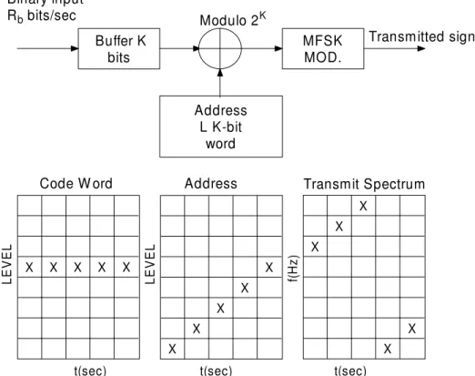
2.1 Transmitter block diagram and signal matrices. The matrices show se-quences of logic levels (code word, address) or frequencies (transmitted spectrum) within the transmitter. . . 6 2.2 Receiver block diagram and signal matrices. The matrices show

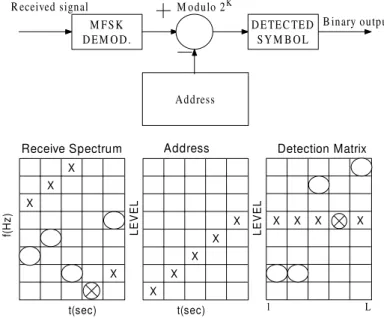
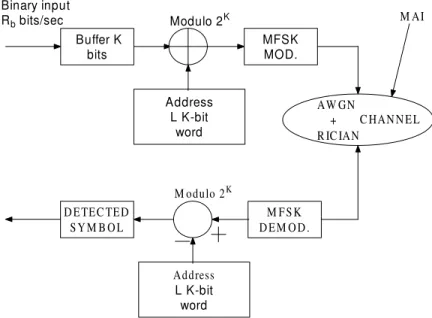
recep-tion of the frequencies in Fig.2.1 (X) and receprecep-tion of a set of tones (O) transmitted by one other user. . . 7 2.3 A block diagram for the FHMA/MFSK system under investigation. . . . 8 2.4 A nonlinear diversity-combining receiver for noncoherent FHMA/MFSK

signals. . . 9 2.5 The effects of a false alarm and a miss on signal in the receiver of 2.2. . . 10 3.1 (Top) the separating hyperplane is not unique; (Bottom) one define a

unique hyperplane corresponding to a maximal distance between the near-est point of the two classes. . . 18 3.2 The margin is the distance between the dashed lines, which is equal to

2/kwk2_{. . . . 19}

3.3 The relation between input space and feature space. . . 24 4.1 Admissible ranges of α2 for the cases α1 + α2 = κ and κ > C (top) or

κ < C (Bottom). . . 32 4.2 Admissible ranges of α2 for the cases α1 − α2 = κ and κ > 0 (top) or

4.3 A DDAG with N = 4 in natural numerical order (top). (Bottom) Due to the frequency of occurrence (1 ≤ 2 < 3 ≤ 4), one may interchange the positions of 2 and 4. . . 37 4.4 The flow chart to implement the proposed SVM-based receivers. . . 38 4.5 Symbol error rate performance of optimum and SVM-based 4FSK

re-ceivers in AWGN channel. . . 39 4.6 Symbol error rate performance of the optimum and SVM-based 4FSK

receivers in AWGN channel and diversity order L = 4. . . 40 4.7 Performance comparison of optimum and SVM-based 4FSK receivers in

Rayleigh fading channels. . . 42 4.8 Performance comparison of Goodman’s and SVM-based 4FSK receivers

in Rayleigh fading channels. . . 43 4.9 Performance comparison of the 4FSK receiver of [17] and SVM-based

receiver in a Rayleigh fading channel with B = 2 and one interferer. . . . 44 4.10 Performance comparison of the 4FSK receiver of [17] and SVM-based

receiver in Rayleigh fading channels with B = 2, η = 1.2 and one interferer. 45 4.11 Performance comparison of SVM-based receivers with different training

Chapter 1

Introduction

Data detection has been casted as a special instant of the hypothesis testing prob-lems. Given an observation vector R, an optimal binary communication receiver makes a decision based on

Λ(R)def= Γ(R) + η def= logp(R|H1) p(R|H0)

+ η (1.1)

where Γ(R) is called the log-likelihood ratio, η is a constant and p(R|Hi), i = 0, 1 is the

conditional probability density function (pdf) of R given that the hypothesis Hi is true.

For the channel model

Hi : R = mi+ W (1.2)

where mi, i = 0, 1, are constant vectors and W is a zero-mean white Gaussian random

vectors, the decision variable Λ(R) is of the form

Λ(R) = a (hR, m1i − hR, m0i) + b (1.3)

where a, b are constants. In case m1 = −m0 = m, we have

Λ(R) = 2ahR, mi + b (1.4)

The inner products hR, mii represent a similarity measure between the received vector

R and the candidate signal mi. A binary decision based on (1.3) or (1.4) is also known as

a binary classifier. In this sense a receiver of a binary communication system is a binary classifier and that of an M -ary communication system can be regarded as a multiple (M ) class classifier.

In many real-world applications, however, the channel model (1.2) is invalid and the conditional pdfs p(R|Hi) do not have a closed-form expression. Moreover, in the space

where the received vector R lies, there might not be a well-defined inner product. For-tunately, recent advances in machine learning have produced many elegant solutions to resolve the above difficulties for binary and M -ary classifiers. There is a major distinc-tion between machine learning and signal detecdistinc-tion in a digital communicadistinc-tion receiver: the latter has very little latency tolerance and real-time processing is an absolute ne-cessity while the former usually requires a reasonable learning period. The purpose of this thesis is to propose a plausible solution to this dilemma so that a receiver can take the advantage of the information extracted from sophisticated statistical learning while requires only simple operations for real-time detection.

The underlying philosophical guideline of our investigation is: we believe that the computing power of digital signal processors has steadily improved for the past two decades to the point that the incorporation of computational intelligence in a wireless communication device has become both feasible and desirable. We envision a commu-nication receiver to possess, besides some stored intelligence, advanced on-line learning capability. This thesis represents a preliminary study towards establishing a theoretical framework for design such an intelligent communication processor.

To demonstrate the powerfulness of our approach, this thesis considers the detection of frequency-hopped multiple access (FHMA) signals in both AWGN and frequency non-selective channels as the sole application example. The same approach can be applied to the detection of a random signal in uncertain environments that do not yield analyt-ical characterization on the associated probability distributions. Multiuser detection of wireless CDMA signals and demodulation of QAM signals in nonlinear satellite channels are but two other candidate applications.

FHMA techniques have been proposed and studied for more than two decades. Cooper and Nettleton [4] first proposed a frequency-hopped, phase-shift-keying,

spread-spectrum system for mobile communication applications. At about the same time Viterbi [22] suggested the use of multilevel FSK (MFSK) for low-rate multiple access mobile satellite systems. In 1979, Goodman et al. [9] studied the capability of a fast frequency-hopped MFSK with a hard-limited diversity combining receiver in additive, white Gaus-sian noise (AWGN) and Rayleigh fading channels.

Two major related design issues concerning the design of an FHMA system are the hopping pattern and the receiver structure. Solomon [15] and Einarsson [6] proposed FH pattern assignment schemes that render minimum multiple assess interference (MAI) in a chip-synchronous environment. Most of the earlier investigations on the noncoherent FHMA receiver design and performance analysis assume that: 1) a single-stage detector is employed by the receiver. 2) a chip(hop)-synchronous mode is maintained, i.e., all users switch their carrier frequencies simultaneously. The second assumption is a more practical assumption for the forward link than for the reverse link. The assumption also exempts the receiver from dealing with cochannel interference (CCI) and interchannel interference (ICI) if an appropriate channel separation is used by the system. Timor [20] proposed a two-stage chip-synchronous demodulator that is capable of eliminating most of the CCI if the thermal noised effect can be neglected by taking advantage of the inherent algebraic structure. He later [21] extended the two-stage demodulator to a multistage decoding algorithm to further improve the system performance. Recently, Su et al. [17] presented a nearly maximum likelihood (ML) diversity combiner for detecting asynchronous FHMA/MFSK signals in Rayleigh fading channels and analyze the perfor-mance of a close approximation of the ML receiver. They also discussed the effectiveness of a two-stage multiuser detector.

Since the relative timing offsets, the signal strengths, the hopping patterns for other system (undesired) users and the number of undesired users are usually unknown to the desired user, it is very difficult if not impossible to obtain a closed-form expression for the posteriori (conditional) probability density function (pdf) associated with a noncoherent

MFSK detector output. The derivation of a maximum likelihood detector is thus out of question under the said scenario. We try to solve the FHMA detection problem from a different perspective.

Regarding the FHMA/MFSK waveform observed at the output of a noncoherent matched-filter bank as a two-dimensional pattern, we then have a multiple-pattern clas-sification problem. Recent advances in machine learning theory has offered a variety of approaches that give very impressive performance. In this thesis, we apply a nonlinear technique called support vector machine (SVM) to provide new solution to the problem of concern. SVM has been used in multiuser detection for CDMA systems [2, 8]. Gong [8] has shown that the SVM scheme has the advantage over many traditional adaptive learning approaches (e.g. the Least Mean Square (LMS) algorithm or the error back-propagation algorithm) in terms of performance, complexity and convergence rate. A major advantage of using SVM is that a nonlinear decision function can be constructed easily by using kernel functions, which is often less complex than nonlinear adaptive and neural network methods.

The rest of thesis is organized as follows. In Chapter 2, we give a brief description of a typical FHMA/MFSK system and present the corresponding signal, channel and receiver model. Chapter 3 contains an overview on the theory of Support Vector Ma-chines(SVM) classifiers. In Chapter 4, we then apply the SVM method to the design of the FHMA/MFSK signal detector and provide some numerical examples of the behavior of our SVM-based receiver. Finally, in Chapter 5, we draw some conclusion remarks and suggest some further works.

Chapter 2

Review of FHMA/MFSK Systems

In this chapter, we examine of the basic building blocks of an FHMA/MFSK system and briefly review the performance analysis of two existing representative receivers. In particular, we consider the receiver proposed by Goodman et al. [9] and that by [17]. For the former case, we assume that: 1) a single-stage detector is employed by the receiver. 2) a chip(hop)-synchronous mode is maintained, i.e., all users switch their carrier frequencies simultaneously. Later, we discuss the signal model, which removes the assumption 2). This chapter is organized as followed. In Section 2.1, we describe the system architecture proposed by Goodman et al. and in Section 2.2, we discuss the corresponding error rate performance. We then consider a modified receiver model [17] that takes into account the effects of ICI and CCI in Section 2.3.

2.1

Basic system building blocks

A block diagram for the transmitter of FHMA/MFSK system is given in Figs. 2.1-2.2. The data source produces a data bit stream of rate Rb = K_T bit/s which is then converted

into a K-bit word sequence {Xm}. The subscript m denotes mth link (user) in a

mul-tiuser system. Each user is assigned an unique signature sequence {am1, am2, · · · , amL}

of rate τ = T_L, where ami ∈ {0, 1, · · · , M − 1} are k−bit symbols and each information

Buffer K bits MFSKMOD. Address L K-bit word Modulo 2K Binary input Rb bits/sec Transmitted signal X X X X X X X X X X X X X X X

t(sec) t(sec) t(sec)

LE V E L LE V E L f(H z)

Code W ord Address Transmit Spectrum

Figure 2.1: Transmitter block diagram and signal matrices. The matrices show sequences of logic levels (code word, address) or frequencies (transmitted spectrum) within the transmitter.

sequence of the same length. The resulting spread symbol sequence {Yml} is given by

Yml = Xm⊕ aml (2.1)

which is then used to select transmitter carrier frequencies.

At the receiving end of the system, demodulation and modulo-M subtraction are performed, yielding

Zml = Ymlª aml = Xm. (2.2)

If there are other users sharing the same frequency band, the received signals could be scattered over different frequency bands at the (desired) mth user’s receiver time-frequency filter outputs. The interference caused by the nth user is

M FSK

DEM OD. DETEC TEDSYM B OL Address M odulo 2K R eceived signal B inary output X X X X X X X X X X X X X t(sec) t(sec) LE V E L LE V E L

Receive Spectrum Address Detection Matrix

1 L

f(H

z)

Figure 2.2: Receiver block diagram and signal matrices. The matrices show reception of the frequencies in Fig.2.1 (X) and reception of a set of tones (O) transmitted by one other user.

If the anl and amlare different, Zml 6= Z

0

ml, i.e., there will be no interference in the desired

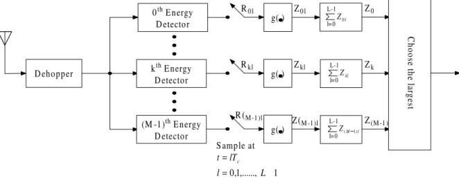
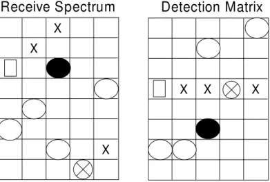
band, see Fig. 2.2 in which crosses denote tones of the mth user while circles denote interfering tones. Using a proper family of signature sequences there will be minimum interfering tones coincided with the desired signal allowing multiple users to access the same frequency band. A block diagram for a complete FHMA/MFSK system is depicted in 2.3. We now address the issue the detecting FHMA/MFSK signals in a multiuser environment. We start with a generic nonlinear diversity-combining receiver as that shown in Fig. 2.4. The received waveform is first dehopped and then detected by a bank of energy detectors before passing through a memoryless nonlinearity g(·). For the one proposed by Goodman et al. [9], g(·) is simply a hard-limiter. Two kinds of error might occur, false alarm and miss. A false alarm occurs when the detected energy is greater than the hard-limiter threshold so that the detector produces an output indicating the presence of a signal tone while there is in fact none. A miss refers to the opposite case when an energy detector produces a “no signal” indicator while signal is actually

Buffer K bits MFSKMOD. Address L K-bit word Modulo 2K Binary input Rb bits/sec M FSK DEM OD. DETEC TED SYM B OL Address L K-bit word M odulo 2K AW GN + R IC IAN C HANNEL M AI

Figure 2.3: A block diagram for the FHMA/MFSK system under investigation.

present. We illustrate the effects of false alarms and misses in Fig. 2.5. The sole square indicates a missing tone in the transmitted code word and the filled circle indicates a false alarm. It is obvious that there is no complete row of “signal present” indicators in the detection matrix. Hence, it is not a good strategy to insist on choosing a complete row as a decision. To allow for this possibility, Goodman et al. use the majority logic decision rule: Choose the code word associated with the row containing the greatest number of “signal present” entries. Under this decision rule, an error will occur when insertions (tones due to other users and false alarms) form a row with more or the same number of entries than the row corresponding to the transmitted code word.

2.2

Error rate analysis

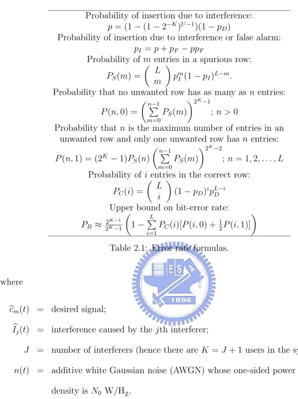
This section mainly follows the derivations of [9]. Table 2.1 contains a set of formulae which give a tight upper bound on the average bit error rate as a function of the following quantities:

Dehopper 0th _Energy Detector kth _Energy Detector (M -1)th Energy Detector g( ) R0l Z0l g( ) Rkl Zkl g( ) R (M-1)l _Z( M-1)l l Z0 Z0 Zk Z(M-1) Sample at 1 ,..., 1, 0 -= = L l lT t c C ho os e t he la rg es t L-1 l=0 kl Z L-1 l=0 l M Z( 1) L-1 l=0

Figure 2.4: A nonlinear diversity-combining receiver for noncoherent FHMA/MFSK signals.

(2) L hopped times per code word. (3) U simultaneous users.

(4) pD miss probability.

(5) pF false alarm probability.

A key assumption in the derivation of these formulas is that the signature sequence of each user is chosen at random. That is, each aml is uniformly distributed between 0 and

2K_{− 1 and is independent of all other address word. For the detail of derivation, please}

refer to [9].

2.3

A nonlinear diversity-combining detector

In this section, we introduce another receiver structure [17] that works for both the chip(hop)-synchronous and chip asynchronous conditions. Without the chip-synchronous assumption different FHMA codewords are no longer orthogonal and interfering system users cause only not co-channel interference (CCI) but also inter-channel interference

X X X

Detection Matrix

X X X

Receive Spectrum

Figure 2.5: The effects of a false alarm and a miss on signal in the receiver of 2.2.

(ICI). In other words, even if an interfering user does not use the same tone during a given hop interval, it still contribute to the desired user’s energy detector output.

Let the L-tuple, a = (a0, a1, . . . , aL−1), be a signature sequence, where, as before,

ai ∈ G = {0, 1, . . . , M − 1}, represents a candidate FSK tone of duration Tc seconds.

The actual transmitted frequencies within a symbol interval is

fm = f0+ (bm0, bm1, . . . , bm(L−1))4f = f0+ (m ⊕ a)4f,

where m = (m, m, . . . , m) is a constant L-tuple representing a K bits message, ⊕ denotes modulo-M addition, f0 is the carry frequency, 4f is the tone space and bml ∈ G. Define

a set of basis waveforms

xnl(t) =

√

SPTc(t − lTc)e

i[2π(f0+bml4f )t] _(2.4)

where S is the signal power, Ec = STc is the average signal energy per chip, Tc = Ts/L

is the chip duration and

PTc(t) =

½

1, 0 ≤ t < Tc

0, otherwise. (2.5)

The received waveform, corresponding to the desired user, consists of three components br(t) = bcm(t) + J X j=1 b Ij(t) + n(t) (2.6)

Probability of insertion due to interference: p = (1 − (1 − 2−K₎U −1_{)(1 − p}

D)

Probability of insertion due to interference or false alarm: pI = p + pF − ppF

Probability of m entries in a spurious row: PS(m) = µ L m ¶ pm I (1 − pI)L−m.

Probability that no unwanted row has as many as n entries: P (n, 0) = µ_n−1 P m=0 PS(m) ¶2K₋₁ ; n > 0

Probability that n is the maximum number of entries in an unwanted row and only one unwanted row has n entries: P (n, 1) = (2K _{− 1)P} S(n) µ_n−1 P m=0 PS(m) ¶2K₋₂ ; n = 1, 2, . . . , L Probability of i entries in the correct row:

PC(i) = µ L i ¶ (1 − pD)ipL−iD

Upper bound on bit-error rate: PB≈ 2 K−1 2K₋₁ µ 1 −PL i=1

PC(i)[P (i, 0) + 1₂P (i, 1)]

¶

Table 2.1: Error rate formulas.

where

bcm(t) = desired signal;

b

Ij(t) = interference caused by the jth interferer;

J = number of interferers (hence there are K = J + 1 users in the system); n(t) = additive white Gaussian noise (AWGN) whose one-sided power spectral

density is N0 W/HZ.

We assume that different MFSK tones at the same chip experience independent and identically (i.i.d) frequency nonselective Rician fading and statistics of a user signal at different chips are i.i.d. as well. Ignoring the propagation delay, the desired signal can be written as bcm(t) = L−1 X l=1 αml √ SPTc(t − lTc)e i[2π(f0+bml4f )t+θml] _(2.7)

where {θml} are random variables (r.v.s) uniformly distributed within [0, 2π) and {αml}

are i.i.d. Rician (r.v.s). Note that {θml} represents the noncoherent receiver’s

uncer-tainty about the phase of the received waveform. Let Γ be the ratio of the power a2_{in the}

specular component to the power, 2σ2

f, in the diffused component. Using the

normaliza-tion, E(α2

ml) = a2+2σf2 = 1, we obtain a2 = Γ/(1+Γ) and 2σ2f = 1/(1+Γ), respectively.

The jth interfering signal, being transmitted through a similar but independent Rician fading channel, has the form

b Ij(t) = M −1_X k=0 L−1 X l=0 αjlcjkl √ SPTc[t − (l − εj)Tc]e i[2π(f0+k4f )t+θjl] _(2.8)

where αjl and θjl are independent random variables having the same distribution as

αml and θml of the desired signal. However, for each (j, l) pair only one cjkl is nonzero,

i.e., cjkl = δ(k − bjl), where δ(x) =

½

1 if x = 0

0 otherwise. and bjl is the frequency tone used by the jth interferer during the lth chip interval. εj is the corresponding normalized

timing misalignment with respect to the desired signal and is assumed to be uniformly distributed with in [0, 1]. With the received waveform given by (2.6)-(2.8), the dehopped signal becomes r(t) = cm(t) + J X j=1 Ij(t) + n(t) (2.9) where cm(t) = L−1 X l=1 αml √ SPTc(t − lTc)e i[2π(f0+m4f )t+φml] _(2.10) Ij(t) = M −1_X k=0 L−1 X l=0 {αjlcjkl √ SPTc[t − (l − εj)Tc]e i[2π(f0+gkl4f )t+φjl] +αj(l+1)cjk(l+1) √ SPTc[t − (l + 1 − εj)Tc]e i[2π(f0+gkl4f )t+φ0_jl] } (2.11)

and gkl = (k − al) mod M . Since the phase of the local frequency synthesizer is not

continuous (noncoherent) when it hops from one band to another, i.e., the “local phases” at different hops are independent, the dehopped random phases, φml, φjl, φ0jl are i.i.d.

imply that perfect power control has been assumed so that all the received signals have the same average strength. Now, we consider the complex random variable Unl, which

is given by Unl = 1 Ec Z (l+1)Tc lTc r(t)x∗_nl(t)dt def= snl+ J X j=1 Ijnl+ znl (2.12) where r(t) is given by (2.9), x∗

nl(t) is the complex conjugate of xnl(t) defined by (2.4),

and snl, Ijnl, znl are the components contributed by the desired signal, the jth interferer

and AWGN, respectively.

Denote the output of the nth energy detector at the jth diversity branch (hop) during a given symbol interval by Rnl (see Fig. 2.4). Then, it can be shown that Rnl = kUnlk2.

In particular, Znl is a zero-mean complex Gaussian random variable whose real and

imaginary parts have the same variance σ2

0 = (2Ec/N0)−1. Substituting (2.4) and

(2.9)-(2.11) into the upper part of (2.12), we immediately have snl = αmleiφmlsinc[(m − n)η]ei[2π(m−n)(l+

1

2)η] (2.13)

where sinc(x) ≡ sin(πx)/(πx), η = 4f/Rc, and

Ijnl = M −1_X

k=0

n

αjlcjkleiφjl(1 − ²j)sinc[gkln(1 − ²j)η]ei[2πgkln(l+

1−εj 2 )η] o + M −1_X k=0 n αj(l+1)cjk(l+1)eiφ 0 j(l+1)²

jsinc[gkln²jη]ei[2πgkln(l+1−

εj 2)η]

o

(2.14) with gkln= gkl−n = [(k−al)mod M ]−n. Although the channel separation gklncan be as

large as M − 1, the corresponding ICI is a decreasing function of the parameter. Hence we will only consider 2B adjacent channels around the desired tone. The magnitude of the product gkln4f represents the frequency separation between the dehopped jth

interferer at the lth hop and the nth energy detector. The term sinc[gkln(1 − εj)η]

represents the contribution to the output of the nth energy detector associated with the kth MFSK tone, which is generated by the jth interferer in the lth chip interval. As shown by (2.14), the orthogonality among the MFSK tones can no longer be maintained,

since the sinc[gkln(1 − εj)η] or sinc[gklnεjη] is nonzero unless εj = 0 or 1 for all j

(chip-synchronization), and, simultaneously η = 4f/Rc is an integer (Rc = 1/Tc is the chip

rate).

2.4

A suboptimal realization

In this section, we discuss the suboptimal receiver proposed by [17]. According to the Bayes’ decision rule, the noncoherent receiver is depicted in Fig.2.4 and the nonlinearity g(x) is given by g(x) = R1/2[gopt(x) − gopt(0)] gopt(R1/2) − gopt(0) (2.15) where gopt(x) ≡ lnfRml(x|m) − fRml(x|k) (2.16)

and fRnl(x|m) is the probability density function under the mth chip is transmitted. It

can be shown that

fRnl(x|m) = 1 2 Z ∞ 0 λJ0(√xλ)ΦXnl(λ|m)dλ (2.17) where X2

nl = Rnl and ΦXnl(λ|m) is the characteristic function of Xnl, which can be given

by ΦXnl(λ|m) = e −λ2_σ2 0/2M (λ, m) B Y ρ=−B [(1 − µ)2+ 2µ(1 − µ)H(λ, ρ) + µ2G(λ, ρ)]J (2.18) where δnm is the Kronecker delta function,

M (λ, m) =    B Q ρ=−B,ρ6=0 n 1 − µ + µe−sinc2(ρη)λ2σf2/2J 0[asinc(ρη)λ] o , m 6= n e−λ2σf2/2J (aλ), m = n H(λ, ρ) = Z 1 0 e−²2sinc2(ρ²η)λ2σf2/2J 0[a²sinc(ρ²η)λ]d² (2.19) G(λ, ρ) = Z 1 0 e−{[1−²]2sinc2[ρ(1−²)η]+²2sinc2(ρ²η)λ2σ2f/2}J 0(a²sinc[ρ²η]λ) J0(a[1 − ²]sinc[ρ(1 − ²)η]λ)d² (2.20)

Furthermore, R1/2 is derived according to gopt(R1/2) = 0.5gopt(Rsat) and the saturation

point Rsat is defined as Rsat = min{x : g0opt(x) = 0}. Since Rsat is often difficult to

locate, we may choose R0

sat = 100d, where d ≡ NE0c, as the reference point and define Rsat

as the value such that gopt(R1/2) = 0.5gopt(R0sat).

However, we can further approximate the soft-limiter by a q-level quantizer, eg(·), with a uniform step size of ν = Υ/(q −1) ≡ R0

sat/(q −1), where Υ is the upper threshold

of the quantizer. In this case, the probability mass function of a uniform quantizer’s outputs {Znl = eg(Rnl)} can be expressed as

PZnl(z) = q−1 X k=0 Pr(Znl = kν)δ(z − kν) ≡ q−1 X k=0 Vnl(k)δ(z − kν)

where the probabilities Vnl(k) = Pr(Znl = kν) = Pr(kν ≤ Rnl < (k + 1)ν) are given by

Vnl(k) =

½

FRnl((k + 1)ν|m) − FRnl(k)ν|m), k = 0, 1, . . . , q − 2

1 − FRnl(Υ|m), k = q − 1

assuming that the mth chip has been transmitted. The cumulative distribution function FRnl(R|m) can be given by FRnl(R|m) = √ R Z ∞ 0 J1( √ Rλ)ΦXnl(λ|m)dλ (2.21) Define

Cnl(k) = Pr{the nth chip output=kν, when the number of diversity branches

used for combining is l + 1 | the mth chip is transmitted} (2.22) Then, we have

Cn(L−1)(k) = Pr(Zn = kν| the mth bin is transmitted) (2.23)

where Zn = L−1_P

l=0

Znl is the output of an L-diversity combiner. The conditional probability

mass function of Zn is given by

PZn =

L(q−1)_X

k=0

With those above equations and the assumption that {Rnl} are approximately i.i.d.

r.v.s, the symbol error probability can be expressed as Ps(M ; L) = 1 − Pr(correct symbol decision)

= 1 − L(q−1)_X k=1 Cm(L−1)(k) M −1_X i=0 µ M − 1 i ¶_[C n(L−1)(k)]i i + 1 "_k−1 X l=0 Cn(L−1)(l) #M −i−1 +Cm(L−1)(0) M £ Cn(L−1)(0)¤ M −1 (2.25)

Chapter 3

Support Vector Machine Classifiers

In this chapter, we give a brief overview on the Support Vector Machines (SVM) classifiers. We discuss linear SVM classifiers with separable and non-separable cases and then extend the results to nonlinear SVM classifiers by using the “kernel trick”. This chapter is organized as follows [19]. After introducing the notion of maximal margin, which is an important concept for understanding SVM, we discuss the linear SVM classi-fiers with separable and non-separable cases. The ensuing section introduces the kernel trick and Mercer condition–a key idea to extend the results from linear to nonlinear. Finally, we explain how to apply the kernel trick to design nonlinear SVM classifiers. For the further readings, please refer to [1, 5, 18, 19]

3.1

Maximal margin

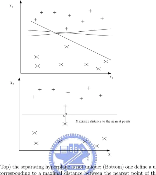
Fig. 3.1 shows a separable classification problem in a two-dimensional space. One can see that there exist several separating lines that completely separate the data of the two classes (labelled by ‘x’ and ‘+’, respectively). It is natural to ask “among these separating lines, which one is the best?” In order to obtain an unique hyperplane, Vapnik suggested rescaling of the problem such that the points closest to the hyperplane satisfy |wT_x

k+ b| = 1, where w is the normal vector of the hyperplane and xk are the closest

points to the hyperplane in the space. The problem can thus be formulated as max

w_∈Rn_,b∈R min{kx − xik |x, xi ∈ R

X1 X2

X1

Maximize distance to the nearest points X2

Figure 3.1: (Top) the separating hyperplane is not unique; (Bottom) one define a unique hyperplane corresponding to a maximal distance between the nearest point of the two classes.

subject to the constraint ½

wT_{x + b > +1 if y}

k = +1

wT_{x + b 6 −1 if y}

k = −1

where yk ∈ {−1, +1} is the output decision or the class label. The constraint can be

rewritten as

yk(wTx + b) > +1

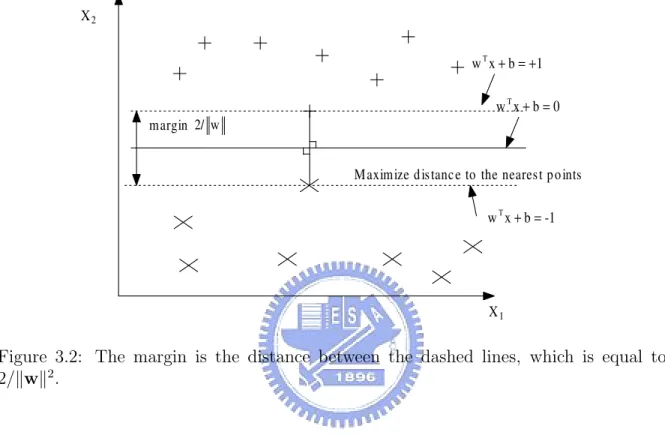
Notice that the margin equals 2/kwk2_{, as illustrated in Fig. 3.2 (kwk}2 _{= w}T_{w). Hence,}

is the hyperplane that maximizes the distance to the nearest points of the two classes. It is obviously that to maximize the distance is equivalent to minimizing kwk2 _subject

to the constraint yk(wTx + b) > +1, which is a convex optimization problem. Such

an optimization problem is mathematical tractable and there exist several well-known algorithms, e.g., the interior point algorithms.

X2

X1

Maximize distance to the nearest points

1 b x wT _{+ =+} 0 b x wT _{+ =} -1 b x wT _{+ =} margin 2/ w

Figure 3.2: The margin is the distance between the dashed lines, which is equal to 2/kwk2_.

3.2

Linear SVM classifiers with separable case

Consider a given training set {xk, yk}Nk=1 with input data xk ∈ Rn, output data yk ∈

{−1, +1} and N is the cardinality of the training point set. As discussed above, a classifier can be regarded as a hyperplane satisfying the maximal margin. The linear classifier can be written as:

y(x) = sign(wTx + b) (3.1)

One would like to have w and b that maximize the margin subject to the constraint that all training samples are correctly classified. This gives the following primal problem

min w_,b JP(w) = 1 2w T_w subject to yk(wTx + b) > +1, k = 1, . . . N

To solve this problem, one introduces the Lagrangian multipliers αk ≥ 0 for k = 1, . . . , N

L(w, b; α) = 1₂wT_{w −}

N

X

k=1

αk(yk(wTxk+ b) − 1) (3.2)

The solution is given by the saddle point of the Lagrangian max

α minw_,b L(w, b; α).

Hence one obtains

∂L ∂w = 0 −→ w = N X k=1 αkykxk (3.3) ∂L ∂b = 0 −→ N X k=1 αkyk = 0 (3.4)

Substituting (3.3) into (3.1), one get y(x) = sign(

N

X

k=1

αkykxTkx + b) (3.5)

By replacing the expression for w (3.3) in (3.2) and using (3.4), one obtains the following Quadratic Programming (QP) problem as the dual problem in the Lagrange multipliers αk max α JD(α) = − 1 2 N P k,l=1 ykylxTkxlαkαl+ N P k=1 αk subject to N P k=1 αkyk = 0

This QP problem has a number of interesting properties: • Sparseness:

An interesting property is that many of the resulting αk values are equal to zero.

Hence the obtained solution vector is sparse. This means that in the resulting classifier the sum should be taken only over the non-zero αk values instead of all

y(x) = sign(

]SV_P k=1

αkykxTkx + b)

where the index k runs over the number of support vectors, which are the training points corresponding to non-zero αk.

• Global and unique solution:

The matrix related to α in this quadratic form is positive definite or positive semidefinite. If the matrix is positive definite (all eigenvalues are strictly positive), the solution α to this QP problem is global and unique. When the matrix is positive semidefinite (all eigenvalues are positive or zero), the solution is global but not necessarily unique. There is another interesting fact: the solution of (w,b) is unique but α may be not. In terms of w = PN

k=1

αkykxk, this seems to mean that

there may exist equivalent expansions of w which require fewer support vectors. • Geometrical meaning of support vectors:

The support vectors obtained from the QP problem are located close to the decision boundary. Notice that the training points located close to the decision boundary may not be support vectors.

• The physical meaning of the support vector [18]

If we assume that each support vector xi exerts a perpendicular force of size αiand

direction yj · w/kwk on a solid plane sheet lying along the hyperplane, then the

solution satisfies the requirements for mechanical stability. The constraint (3.4) states that the forces on the sheet sum to zero, and (3.3) implies that the torques also sum to zero, via P_ixi× yiαiw/kwk = w × w/kbfwk

3.3

Linear SVM classifiers with nonseparable case

Most real-world problems that one encounters are nonseparable either in a linear sense or nonlinear sense. For example, consider the classical detection problem: one transmits

a signal x ∈ {−1, +1} and the received signal is y = x + w, where w is AWGN. It is well-known that the optimal decision boundary is a linear separating hyperplane according to Bayesian decision theory; see Chapter 1. Linear non-separability is most likely a result of overlapping distributions. For the class of linearly nonseparable cases (with overlapping distributions between the two classes), one is forced to tolerate misclassifications. It is done by taking additional slack variables in the problem formulation. In order to tolerate misclassifications, one modifies the set of inequalities as

yk(wTx + b) > 1 − ξk, k = 1, . . . , N

with the slack variables ξk ≥ 0. When ξk > 1, the kth inequality becomes violated in

comparison with the corresponding inequality of the linearly separable case; that is, it is a misclassified point. In the primal weight space the optimization problem (primal problem) becomes: min w_,b,ξJP(w, ξ) = 1 2w T_{w + C} PN k=1 ξk subject to yk(wTxk+ b) ≥ 1 − ξk, ξk ≥ 0 k = 1, . . . , N

where C is a positive real constant. The following Lagrangian are to be considered L(w, b, ξ; α, ν) = JP(w, ξ) − N X k=1 αk(yk(wTxk+ b) − 1 + ξk) − N X k=1 νkξk (3.6)

with Lagrange multipliers αk ≥ 0, νk ≥ 0 for k = 1, . . . , N. The second set of Lagrange

multipliers is needed due to the additional slack variables ξk. The solution is given by

the saddle point of the Lagrangian: max α,ν minw_,b,ξL(w, b, ξ; α, ν) One obtains ∂L ∂w = 0 −→ w = N X k=1 αkykxk (3.7) ∂L ∂b = 0 −→ N X k=1 αkyk= 0 (3.8) ∂L ∂ξk = 0 −→ 0 ≤ α k ≤ c, k = 1, . . . , N (3.9)

By replacing the expression for w (3.7) in (3.6) and using (3.8), one obtains the following dual QP problem: max α JD(α) = − 1 2 N P k,l=1 ykylxTkxlαkαl+ N P k=1 αk subject to N P k=1 αkyk = 0 0 _{≤ α}k≤ c, k = 1, . . . , N

3.4

Kernel, Kernel trick and Mercer condition

In order to extend the linear method to deal with more general cases which often require nonlinear classifiers, one maps an input data vector x into ϕ(x) in a high (can be infinite) dimensional feature space H. It is hopped that the transformed data will be linearly separable in the high dimensional feature space. The constructed separating hyperplane in H may be a nonlinear in the original input space (Fig. 3.3).

It is indeed possible that no explicit specification of the nonlinear mapping ϕ(x) is needed when constructing the separating hyperlane. This is due to the following theorem which leads to the concept of kernel trick.

Theorem 1 For any symmetric, continuous function K(x, z) satisfying the Mercer’s condition

Z

ZK(x, z)g(x)g(z)dxdz ≥ 0

(3.10) for any square integrable function g(x), where Z is a compact subset of Rn_{, there exists}

a Hilbert space H, a map ϕ : Rn_{−→ H and positive numbers λ}

i such that K(x, z) = nH X i=1 λiϕi(x)ϕi(z) (3.11) where x, z ∈ Rn _{and n} H≤ ∞ is the dimension of H.

X2 X1 ) x ( 2 j ) (× j ) x ( 1 j

Figure 3.3: The relation between input space and feature space.

Notice that (3.11) can be rewritten as K(x, z) = nH X i=1 p λiϕi(x) p λiϕi(z) (3.12)

One can define ˜ϕi(x) =√λiϕi(x) and ˜ϕi(z) =√λiϕi(z) so that an inner product in the

feature space is equivalent to the kernel function K(x, z) in the input space

h ˜ϕ(x), ˜_{ϕ(z)i = ˜}ϕ(x)Tϕ(z) = K(x, z).˜ (3.13) Hence, having a positive semidefinite kernel (one satisfies (3.10) is a condition to guar-antee that one can compute the kernel of the input data vectors x, z without the need to construct ϕ(·). In other words, it is possible to find the separating hyperplane without explicitly performing the nonlinear mapping. The application of (3.13) is often called the kernel trick. It enables one to work in high dimensional feature spaces without actually having to do explicit computations in this space.

There are several choices for the kernel K(·, ·). Some typical choices are

K(x, xk) = xTxk (linear SVM) (3.14a)

K(x, xk) = (τ + xTxk)d (polynomial SVM of degree d) (3.14b)

K(x, xk) = exp(−kx − xkk2/σ2) (RBF kernel) (3.14c)

The Mercer condition holds for all σ in the RBF kernel case and all τ > 0 in the polynomial case but not for all possible choices of κ1, κ2 in the MLP kernel case.

It is worth noticing that one can create kernels from kernels. The main idea is to perform some operations on positive definite kernels such that the results still remain positive definite. For symmetric positive definite kernels the following operations are allowed [5]: • K(x, z) = aK1(x, z) (a > 0) • K(x, z) = K1(x, z) + b (b > 0) • K(x, z) = xT_{P z (P = P}T _{> 0)} • K(x, z) = K1(x, z) + K2(x, z) • K(x, z) = K1(x, z)K2(x, z) • K(x, z) = f(x)f(z) • K(x, z) = K1(φ(x), φ(z)) • K(x, z) = p+(K1(x, z)) • K(x, z) = exp(K1(x, z)) where a, b ∈ R+_{and K}

1, K2 are symmetric positive definite kernel functions, f (·) : Rn →

R, φ(·) : Rn_{→ R}nH _{and p}

+(·) is a polynomial with positive coefficients.

One may also normalize kernels: e

K(x, z) = p K(x, z)

K(x, x)pK(z, z) = cos(θϕ(x),ϕ(z)) (3.15)

where eK is the normalized kernel and θϕ(x),ϕ(z) is the angle between ϕ(x), ϕ(z) in the

3.5

Nonlinear SVM classifiers

The extension from linear SVM classifiers to nonlinear SVM classifiers is straightforward. As discussed in section 3.4, one maps the input data into a high dimensional feature space. It means that one replaces x by ϕ(x). Therefore, the primal problem for nonlinear SVM classifiers with nonseparable case is:

min w_,b,ξJP(w, ξ) = 1 2w T_{w + C} PN k=1 ξk subject to yk(wTϕ(xk) + b) ≥ 1 − ξk (3.16) ξk ≥ 0 k = 1, . . . , N (3.17)

and the representation of nonlinear classifier is :

y(x) = sign(wTϕ(x) + b) (3.18)

One should note that the dimension of w is nH, not n (the dimension of the input

space). As discuss in section 3.4, nH can be infinite in general. It means that it is hard

or even impossible to solve the primal problem for large nH. Fortunately, one can solve

this problem by considering the dual problem. Similar to the work in section 3.3, one introduces the Lagrangian multipliers:

L(w, b, ξ; α, ν) = JP(w, ξ) − N X k=1 νkξk− N X k=1 αk(yk(wTϕ(xk) + b) − 1 + ξk) (3.19)

with Lagrange multipliers αk ≥ 0, νk ≥ 0 for k = 1, . . . , N. The solution is given by the

saddle point of the Lagrangian: max

One obtains ∂L ∂w = 0 −→ w = N X k=1 αkykϕ(xk) (3.20) ∂L ∂b = 0 −→ N X k=1 αkyk= 0 (3.21) ∂L ∂ξk = 0 −→ 0 ≤ α k ≤ c, k = 1, . . . , N (3.22)

By replacing the expression for w(3.20) in (3.19) and using (3.21), one obtains the following dual QP problem:

max α JD(α) = − 1 2 N X k,l=1 ykylK(xk, xl)αkαl+ N X k=1 αk (3.23) subject to N P k=1 αkyk = 0 0 _{≤ α}k≤ c, k = 1, . . . , N

Then, the nonlinear classifier becomes (substitute (3.20) into (3.18)): y(x) = sign(PN

k=1

αkykK(xk, x) + b)

Notice that the computation is in the input space, and the dimension of the input space is usually finite and not very large. Therefore, one can solve this problem in dual space while can not in primal space.

As denoted in section 3.2, this QP problem has a number of interesting properties: • Sparseness:

As discussed before, many αk values are equal to zero. Hence the obtained solution

vector is sparse. This means that in the resulting classifier the sum should be taken only over the non-zero αk values instead of all training data points as in the linear

case:

y(x) = sign(

]SV_P k=1

where the index k runs over the number of support vectors. • Global and unique solution:

As in the linear SVM case, the solution to the convex QP problem is global and unique if one choose a positive definite kernel. This choice guarantees that the matrix involved in the QP problem is positive definite and that one can apply kernel trick as well.

• Geometrical meaning of support vectors:

The support vectors obtained from the QP problem are located close to the decision boundary. Notice that the training points located close to the decision boundary may not be support vectors.

Chapter 4

Detector Structures Based on SVM

Techniques

Two critical issues arise when applying the SVM scheme to solve our detection problem, namely, the training speed and the multi-class classification issues. We will describe a fast algorithm for training support vector machine–the Sequential Minimal Optimization (SMO) algorithm. This algorithm breaks a large QP optimization problem into a series of smallest possible QP tasks. These small QP tasks are solved analytically, which avoids using a time-consuming numerical QP optimization as an inner loop. We then discuss the Directed Acyclic Graph (DAG) method that combines many two-class classifiers into a multi-class classifier. For an N -class problem, the DAG contains N (N − 1)/2 classifiers, one for each pair of classes.

By applying the DAG algorithm to classify the computer generated training samples and using the SMO algorithm, we obtain the support vectors for binary classification. Given these support vectors, we then apply the DAG method for real-time signal detec-tion. Thus the design of a SVM-based FHMA/MFSK detector requires an off-line (non-real time) training period to find the associated support vectors. Once these support vectors become available, we place them in the detector memory and on-line detection just follows a predetermined DAG algorithm using the known support vectors. Before giving numerical application examples, we summarize the major attributes of SMO and DAG algorithms in the following sections.

4.1

The SMO Algorithm

The architecture of the SMO algorithm can be summarized as follows. M1. The outer loop: select the first Lagrange multipliers to be optimized. M2. The inner loop: select the second Lagrange multipliers to be optimized. M3. Solving for two selected Lagrange multipliers analytically.

We now proceed to address [SMO3] and then [SMO1] and [SMO2], respectively.

4.1.1

Analytical Lagrange multiplier solutions

Each step of SMO will optimize two Lagrange multipliers. Without loss of generality, let us denote these two multipliers by α1 and α2, respectively. The objective function

(3.23) can be rewritten as min α JD(α) = 1 2 N X k,l=1 ykylK(xk, xl)αkαl− N X k=1 αk = 1 2K11α 2 1+ 1 2K22α 2 2+ y1y2K12α1α2+ y1α1v1+ +y2α2v2−α1−α2+ residual terms (3.1) where Kij = K(xi, xj) vi = N X j=3 yjα∗jKij = ui− b∗− y1α∗1K1i− y2α∗2K2i ui = N X j=1 yjα∗jKj,i+ b∗

and the starred variables indicate the values at the end of the previous iteration. For the initial state, one can start with α∗

i = 0 for i = 1, . . . , N . Residual terms do not depend

on either α1 or α2. From (3.21), we obtain

where s = y1y2. Then (3.1) can be represented in terms of α2 only. JD = 1 2K11(κ − sα2) 2₊ 1 2K22α 2 2+ sK12(κ − sα2)α2+ y1(κ − sα2)v1 +y2α2v2− (κ − sα2) − α2 + residual terms (3.3)

The first and second derivatives are given by dJD dα2 = −sK11(κ − sα2 ) + K22α2− K12α2 +sK12(κ − sα2) − y2v1+ s − 1 + y2v2 (3.4) d2_J D dα2 2 = K11+ K22− 2K12= η (3.5)

Notice that η ≥ 0 if K(·, ·) satisfies the Mercer’s condition. (3.4) can be rearrange as: α2η = α∗2η + y2(E1− E2) =⇒ αnew2 = α∗2+

y2(E1− E2)

η (3.6)

where Ei = ui− yi. Because 0 ≤ α2 ≤ C, we need to check the admissible range of α2,

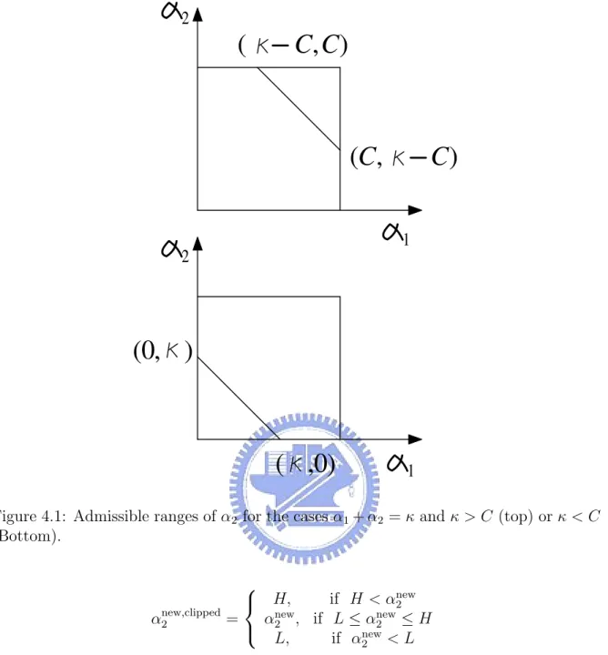
which is determined by the following rules: • If s = 1, then α1+ α2 = κ (Fig. (4.1))

– If κ > C, the max of α2 = C and the min of α2 = κ − C

– If κ < C, the max of α2 = κ and the min of α2 = 0

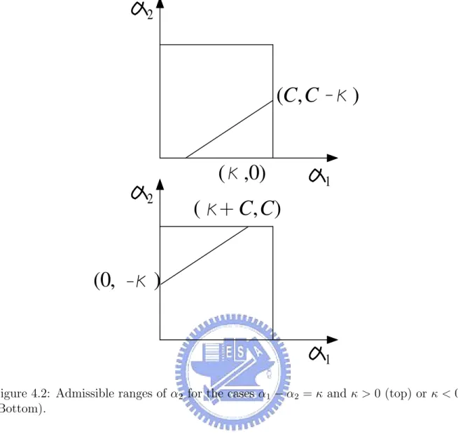
=⇒ L = max(0, κ − C) and H = min(C, κ). • If s = −1, then α1− α2 = κ (Fig. (4.2))

– If κ > 0, the max of α2 = C − κ and the min of α2 = 0

– If κ < 0, the max of α2 = C and the min of α2 = −κ

=⇒ L = max(0, −κ) and H = min(C, C − κ). Hence, we have

)

,

(

C

C

)

,

(

C

C

)

0

,

(

)

,

0

(

1

2

1

2

Figure 4.1: Admissible ranges of α2 for the cases α1+ α2 = κ and κ > C (top) or κ < C

(Bottom). αnew,clipped₂ =    H, if H < αnew 2 αnew 2 , if L ≤ αnew2 ≤ H L, if αnew 2 < L

To summarize, given α1, α2 (and the corresponding y1, y2, K11, K12, K22, E1 − E2), we

optimize the two α’s by the following procedure: O1. Letη = K11+ K22− 2K12.

O2. If η > 0, set

4α2 = αnew2 − α∗2 =

y2(E1− E2)

)

0

,

(

)

,

( C

C

)

,

(

C

C

)

,

0

(

1

1

2

2

Figure 4.2: Admissible ranges of α2 for the cases α1− α2 = κ and κ > 0 (top) or κ < 0

(Bottom).

and clip the solution within the admissible region (αnew,clipped₂ ) so that

4α1 = −s4α2 (3.8)

O3. If η = 0, we need to evaluate the objective function at the two endpoints and set αnew

2 to be the one with smaller objective function value. The objective function

is given by (See Appendix A)

JD = 1 2ηα 2 2+ (y2(E2− E1) − α2∗η)α2+ Const. (3.9) .

4.1.2

Choices of the Lagrange Multipliers

Consider the KKT (Karush-Kuhn-Tuker) conditions of the primal problem which will be used in picking two Lagrange multipliers stage. The conditions are

∂L ∂w = 0 −→ w = N X k=1 αkykϕ(xk) (3.10) ∂L ∂b = 0 −→ N X k=1 αkyk = 0 (3.11) ∂L ∂ξk = 0 −→ 0 ≤ αk≤ C, k = 1, . . . , N (3.12) αk(yk(wTϕ(xk) − b) + ξk− 1) = 0 k = 1, . . . , N (3.13) νkξk = 0 k = 1, . . . , N (3.14) which imply αi = 0 =⇒ yi(wTxi− b) ≥ 1 0 < αi < C =⇒ yi(wTxi− b) = 1 αi = C =⇒ yi(wTxi− b) ≤ 1

The heuristics for picking two αi’s for optimization are as follows [13]:

• The outer loop selects the first αi, the inner loop selects the second αi that

maxi-mizes |E2− E1|.

• The outer loop alternates between one sweep through all examples and as many sweeps as possible through the non-boundary examples, selecting the example that violates the KKT condition. Once a violated example is found, a second multiplier is chosen using the second choice heuristic, and the two multipliers are jointly optimized. Then, the SVM is updated according to these two new multipliers, and the outer loop continue to find other violated examples.

• Given the first αi, the inner loop looks for a non-boundary that maximizes |E2−E1|.

examples, starting at a random position; if the fails too, it starts a sequential scan through all the examples, also starting at a random position. If all of above fail, the first αi is skipped and the inner loop will continue with another chosen first αi

from outer loop.

4.1.3

Update step

Given the incremental changes 4α1, 4α2, we update the corresponding Ei’s, and b

accordingly. Let E(x, y) be the prediction error of (x, y) E(x, y) =

N

X

i=1

αiyiK(xi, x) + b − y (3.15)

The corresponding variation of E is

4E(x, y) = 4α1y1K(x1, x) + 4α2y2K(x2, x) + 4b (3.16)

The change in the threshold can be computed by forcing Enew

1 = 0, if 0 < αnew1 < C,

or Enew

2 = 0, if 0 < αnew2 < C). The reason for forcing E1 = 0 is that if 0 < α1 < C,

the output of SVM is y1 when the input is x1 (from the KKT conditions) and by the

definition of E1, E1 = 0. From

0 = E(x, y)new

= E(x, y)old_{+ 4E(x, y)}

= E(x, y)old_{+ 4α}1y1K(x1, x) + 4α2y2K(x2, x) + 4b (3.17)

where x = x1 if 0 < α1new< C and x = x2 if 0 < αnew2 < C. Hence, we obtain

−4b = E(x, y)old+ 4α1y1K(x1, x) + 4α2y2K(x2, x) (3.18)

If both α1, α2 are equal to 0 or C, we compute two values of the new b for α1 and α2

using (3.18), and take the average. Notice that if 0 < αnew

i < C for i = 1, 2, the 4b will

4.2

Directed Acyclic Graph (DAG) Algorithm

In general, there are two types of approaches for multi-class SVM:

D1. Construct a multi-class classifier by combining several binary classifiers.

D2. Construct a multi-class classifier by solving one optimization problem with all classes [19].

In this section, we focus on Approach D1 and present the DAG algorithm for the multi-class problems. We first describe two multi-multi-class algorithms (1-v-r and Max-Wins) for comparison, and then give the details of the DAG algorithm and discuss some results about DAG algorithm.

1-v-r (abbreviation for one-versus-the rest) is a standard method for N -class SVMs. It constructs N SVMs with the i-th SVM trained by all of the data and the labels of data changed according to

yi =

½

1 data is in the i-th class

−1 otherwise.

The output is determined by the index (i) of yi = 1.

Max-Wins constructs N (N −1)₂ SVMs with each SVM trained on only two out of N classes. This class of SVMs are often referred to as one-verse-one (1-v-1 ) SVMs in multi-class problems. For combining these binary SVMs, each SVM casts one vote for its preferred class, and the final result is the class with the majority votes.

Before discussing the DAG algorithm, we need to introduce the notion of DAG and Decision DAG (DDAG). A DAG, as the name implies, is a graph whose edges have an orientation but form no cycles. A rooted DAG has a unique node (rooted node) which there is no edge pointing into it. A binary DAG is a graph in which every node has either 0 or 2 edges leaving it. A DDAG is a rooted binary DAG with N leaves labelled by the classes. At each of the N (N −1)₂ internal nodes in a DDAG, a Boolean decision is made. The nodes are arranged in a triangle-like shape in which the i-th node in layer

j < N is connected to the ith and (i + 1)th node in the j + 1th layer. A typical DDAG with N = 4 is illustrated in Fig. 4.3. It is straight froward to use the DAG algorithm for

1 vs 4 2 vs 4 1 vs 3 2 vs 3 1 vs 2 3 vs 4 4 3 2 1 not 4 not 3 not 2 _{not 4} not 1 not 1 1 vs 2 2 vs 4 1 vs 3 3 vs 4 1 vs 4 2 vs 3 2 3 4 1 not 2 not 3 not 4 _{not 2} not 1 not 1

Figure 4.3: A DDAG with N = 4 in natural numerical order (top). (Bottom) Due to the frequency of occurrence (1 ≤ 2 < 3 ≤ 4), one may interchange the positions of 2 and 4.

SVM: using two-class maximal margin hyperplanes at each internal node of the DDAG. In general, we refer this implementation as DAGSVM algorithm for emphasizing SVM. The choices of the class order in the DDAG is arbitrary. One possible heuristic is to place the most frequent classes in the center, as illustrated by Fig.4.3. Yet, reordering the order does not yield significant changes in accuracy performance. Also, It has been experimentally shown that the DAGSVM algorithm is faster to train or evaluate than

either the 1-v-r or Max-Wins, while maintaining comparable accuracy to both of these algorithms [12]. O ff-line Step 1 C onstruct a Decision Directed Acyclic Graph(DDAG). Step 2

Run the SM O algorithm at each internal node of D D AG and store the support vectors.

Step 3

Use the results in step 2 to identify the received

signals.

Figure 4.4: The flow chart to implement the proposed SVM-based receivers.

To implement the proposed SVM-based receivers, there are three steps, as illustrated by Fig. 4.4.

S1. Construct a decision directed acyclic graph(DDAG).

S2. At each internal node of the DDAG, one uses the SMO algorithm to find the two-class maximal margin hyperplane and store the support vectors(SVs).

S3. Use the stored SVs, the SVM-based receiver can identify the received signals. Note that the step 1. and step 2. can be carried out off-line. It can, therefore, save the test period.

4.3

Numerical Examples and Discussion

Unless otherwise specified, all SVM-based receivers use the RBF kernel with σ = 0.5 and the following system parameters are assumed in all the examples given in this section: M = 4, L = 1, U = 1, and η = 1. The reason to choice the RBF kernel is due to the fact that it has been proved that this kernel is universal, which means that linear combinations of this kernel computed at the data points can approximate any function[11].

Example 1 4FSK in AWGN channels.

0 1 2 3 4 5 6 7 8 9 10 10−5 10−4 10−3 10−2 10−1 100 4FSK in AWGN channel Eb/N0 SER Linear kernel Theorical result RBF kernel

Figure 4.5: Symbol error rate performance of optimum and SVM-based 4FSK receivers in AWGN channel.

Fig. 4.5 reveals that a receiver based on the SVM technique can provide performance very close to that achieved by a conventional optimal MFSK receiver. More specifically,

the probability of symbol error for the optimal noncoherent M -ary orthogonal signal detector is given by [16] PM(e) = M −1_X n=1 (−1)n+1 µ M − 1 n ¶ 1 n + 1exp · −nlog2M n + 1 Eb N0 ¸ (3.19) The receiver whose performance is given by the dashed curve uses RBF kernel, 600 training samples and C = 1. The solid one with linear kernel, 600 training samples and C = 6 is plotted as well. The circle points are calculated according to (3.19). Both receivers yield almost the same performance as that of the optimum receiver.

Example 2 4FSK in a single-user AWGN channel with diversity order L = 4.

0 2 4 6 8 10 12 10−6 10−5 10−4 10−3 10−2 10−1 100

4FSK with L=4 in AWGN channel

Eb/N0

SER

Union bound Receiver based on SVM

Figure 4.6: Symbol error rate performance of the optimum and SVM-based 4FSK re-ceivers in AWGN channel and diversity order L = 4.

In Fig. 4.6, we plot the performance curves for the SVM-based receiver and the optimal noncoherent 4FSK receiver. The performance of the latter is computed by using

the union bound [16] for general M -ary orthogonal signal with diversity L. PM(e) < (M − 1)P2(e; L) (3.20) where P2(e; L) = 1 22L−1e −krb₂ L−1 X n=0 cn( 1 2krb) n _(3.21) and cn = 1 n! L−1−n_X k=0 µ 2L − 1 k ¶ (3.22) rb being the SNR per bit and k = log2M .

The solid line corresponds to the performance obtained with 600 training samples and C = 0.9. It is obvious that the performance is almost identical to that of the ideal noncoherent 4FSK receiver except in low SNRs. It is known that [16], for relatively small values of M , the union bound is sufficiently tight for most practical applications. We conclude that the MFSK receiver based on SVM can offer performance very close or identical to the optimal receiver when diversity reception is involved.

Example 3 4FSK in Rayleigh fading channels.

As shown in Fig. 4.7, the performance of the proposed receiver is similar to that of the conventional optimal receiver (matched filter). The solid curve is the SER performance of the SVM-based receiver with 1800 training samples and C = 0.9. Again, we can see that the proposed SVM-based receiver provides performance identical to that of the conventional optimal receiver.

Example 4 4FSK in frequency nonselective Rayleigh fading channels with diversity or-der L = 4.

The SVM-based receiver is obtained with 1800 training samples and C = 0.1. The threshold b is chosen to be q_{2 ∗ (1 +} 1

SN R)ln(1 + SN R) ∗ N0 according to [14].

The solid curve in Fig.4.8 represents the performance of the receiver proposed by Goodman et al. [9] and the dashed curve is the performance of our SVM-based receiver. In this case our receiver outperforms Goodman’s, which is only a suboptimal receiver.

0 2 4 6 8 10 12 14 16 18 20 10−3 10−2 10−1 100 4FSK in Rayleigh channel Eb/N0 SER Receiver based on SVM Conventional receiver

Figure 4.7: Performance comparison of optimum and SVM-based 4FSK receivers in Rayleigh fading channels.

Example 5 4FSK in a Rayleigh fading channel with diversity order L = 4, B = 2 and two system users.

The dashed curve in Fig.4.9 is the performance of our SVM-based receiver. The proposed receiver is achieved with 1800 training samples and C = 0.1. The solid line is the performance of the receiver proposed by [17] with q = 8. It is clear from Fig. 4.9 that our proposed receiver outperform that in [17] too.

Example 6 4FSK in Rayleigh fading channels with diversity order L = 4, B = 2, η = 1.2 and two system users (one interferer).

The dashed line in Fig.4.10 is the performance of our SVM-based receiver. The proposed receiver is obtained with 1800 training samples and C = 0.1. The solid line is

0 2 4 6 8 10 12 14 16 10−4

10−3

10−2

10−1

100 4FSK with L=4 in Rayleigh channel

Eb/N0

SER

Receiver proposed by Goodman Receiver based on SVM

Figure 4.8: Performance comparison of Goodman’s and SVM-based 4FSK receivers in Rayleigh fading channels.

the performance of receiver proposed in [17] with q = 8. Again, Fig. 4.10 shows that our proposed receiver outperforms that in [17].

Example 7 Robustness of SVM-based detectors

In this example, it is illustrated by Fig. 4.11 that SVM may be insensitive to the param-eter: Eb/N0. The solid line is the performance under the SVM receiver whose support

vectors are obtained with the assumption Eb/N0 = 20 dB but are used for different

Eb/N0s. The dashed line, on the other hand, represents the performance of the SVM

receiver using Eb/N0-dependent (optimized) support vectors.

The fact that both receivers yield almost identical performance indicates that the proposed SVM-based receiver is relatively robust against changing Eb/N0. Such robust

0 5 10 15 20 25 10−2

10−1

100 4FSK B=2 with one interferer in Rayleigh channel

Eb/N0

SER

Nonlinear receiver Receiver based on SVM

Figure 4.9: Performance comparison of the 4FSK receiver of [17] and SVM-based receiver in a Rayleigh fading channel with B = 2 and one interferer.

behavior also simplifies our receiver design for there is no need to store different sets of SVs for different Eb/N0s.

0 5 10 15 20 25 10−2

10−1

100 4FSK B=2 eta=1.2 with one interferer in Rayleigh channel

Eb/N0

SER

Receiver based on SVM Nonlinear receiver

Figure 4.10: Performance comparison of the 4FSK receiver of [17] and SVM-based re-ceiver in Rayleigh fading channels with B = 2, η = 1.2 and one interferer.

0 5 10 15 20 25 30 35 40 10−2

10−1

100 4FSK with B=2, one interferer in Rayleigh channel

Eb/N0

SER

SVM trainned in Eb/N0=20dB SVM trainned with different Eb/N0

Figure 4.11: Performance comparison of SVM-based receivers with different training ways.

Chapter 5

Conclusion and Future Works

5.1

Conclusion

This thesis documents our investigation results on the design of receiver based on SVM for MFSK/FHMA system. From the simulation results, we may infer that the receiver based on SVM can approximate to the optimal receiver or outperform proposed receivers in chapter 2. The main reason is due to the fact that the conditional probability density is intractable. The SVM-based receiver, however, does not require the knowledge and usually the performances can approximate to the ML results. Also, the SVM-based receiver is insensitive to the parameter: Eb/N0. With this property, we can save the

memory and implement the receiver without sorting other results based on different Eb/N0.

5.2

Future Works

There are several problems need to be addressed in this technique and we hope we can solve them in the future.

(1.) The channel state may not be static, i.e. the channel model may be time-varying. In this case, the SVM techniques proposed here may not be used directly due to the SMO algorithm and the QP problems.

This is due to the SMO and DAG algorithm and it may be better to solve the QP problem once at all or to handle the training set in advance.

In practice, the size of M will be large. For instance, in [9], it set M = 256. Also, when we apply this technique to Flash-OFDM, this problem will appear again. (3.) In this thesis, we do not indicate the optimal kernel and the choice of parameter

given kernel. We believe that the problem is ongoing research for the moment. (4.) To combine the SVM-based receiver with error correction code will appear some

problems. One of them is the size of M , which is discussed in (2). For instant, the size of M may be 204 for RS(204, 188). Another is the soft input for the error correcting decoder. In our thesis, the output of the receiver is one of {1, 2, 3, . . . M}. It could not be used to be the soft input of the decoder directly. In this case, it may rely on the notion of regression, which is out of scope here.

Appendix A

The Objective Function for SMO

Algorithm

In the section, we derive the (3.9). By SMO algorithm, one can break a large QP problem into a series of smallest possible QP problems, and the smallest possible QP problem can be solved analytically, which avoids using a time-consuming numerical QP optimization as an inner loop. Also, the matrix computation is avoided, so the amount of memory required for SMO is reduced. Hence, one can solve a large QP problem efficiently.

In this algorithm, since the η = 0 is possible, one need some other steps to make the algorithm work. In those steps, one need to know the equation (3.9). Hence we derive the equation for completing the SMO algorithm here.

We begin these deductions with equation (3.3).

JD = 1 2K11(κ − sα2) 2₊1 2K22α 2 2+ sK12(κ − sα2)α2+ y1(κ − sα2)v1 +y2α2v2− (κ − sα2) − α2+ residual terms = 1 2(K11+ K22− 2K12)α 2 2 + (−K11κs + sK12κ − y1sv1+ y2v2+ s − 1)α2 +1 2K11κ 2_{+ y} 1κv1− κ + residual terms (3.1) where vi = N P j=3 yjαj∗Kij = ui− b∗− y1α1∗K1i− y2α∗2K2i