Nonlinear adaptive backstepping motion control of linear induction motor

Proceedings of the American Control Conference Anchorage, AK May 8-1 0,2002

Nonlinear Adaptive Backstepping Motion

Control

of

Linear Indcution Motor

Chin-I Huang',Chen, KO-LO', Hou-Tsan Lee' and Li-Chen Fu'** Department of Computer Science and Information Engineering

National Taiwan University, Taipei, Taiwan, R.O.C.

Department

of

Electrical Engineering

e-mail

:

lichen@csie.ntu.edu.tw

Abstract

In this paper, we will propose a nonlinear adaptive controller and an adaptive backstepping controller for linear induction motol(L1M) to achieve speedposition tracking. A nonlinear transformation is proposed to facilitate controller design. Besides, the very unique end effect oftheLIM is also considered and is well taken care of in our controller design. Stability analysis based on Lyapunov theory is also performed to guarantee that the antroller design here is stable. Also, the computer simulations and experiments are done to demonstrate the performance of our various controller design.

K e p o r d : Nonlinear Adaptive control, Motion Control, Linear Induction motor,Adaptive Backstepping control

Nomenclature

L

INTRODUCTION

Nowadays, LIMs are now wi,dely used, in many industrial applications including transportation, conveyor systems, actuators, material handling, pumping of liquid metal, and sliding door closers, etc. with satisfactory performance. The most obvious advantage of linear motor is that it has no gears and requires no mechanical rotary-to-linear converters. The linear electric motors can be classified into the following: D.C. motors, induction motors, synchronous motors and stepping motors, etc. Among these, the LIM has many advantages such as simple structure replacement of the gear between motor and motion devices, reduction of mechanical losses and the size of motion devices, silence, high starting thrust fbrce, and easy maintenance, repairing and replacement.

In the early works, Yamamura has first discovered a particular phenomenon of the end effect on LIM [I]. A control method, decoupling the control of thrust and the attractive force of a LIM using a space vector control inverter, was presented in

PI,

i.e. by selecting voltage

vectors of PWM inverters appropriately.

Although h e parameters of the simplified equivalent circuit model of a n LIM can be measured by conventional methods (no-load and locked secondary tests), due to limited length of the machine the realization of the no-load test is almost impossible. Thus, the applicability of conventional methods for calculating the parameters of the equivalent model is limited. In order to measure the parameters, application of the finite element (FE) method for determining the parameters of a two-axis model of a three-phase LIM has been proposed in

PI.

Another method is proposed by removing the secondary [4].

To resolve the unique end effect problem, speed dependent scaling factors are introduced to the magnetizing inductance and series resistance in the &axis equivalent circuit o f the rotary induction motor (RIM) [SI. to correct the deviation caused by the "end effect". On the other hand, there is a thrust correction coefficient introduced by [6,7] t o calculate an actual thrust to compensate for the end effect. A related method to deal with the problem is that an extemal force corresponding to the end effect is introduced into the RIM model to provide a more accurate modeling of an LIM

under consideration of end effect as shown in [ 81. In another work [ 9 ] , extra compensating-winding was proposed to compensate such problem.

Although the end effect is an important issue of the LIM control, but there are still many works in the literature without considering it, such as [1@16]. In thispaper, we will take this as an important issue which can not be ignored.

The paper is organized as follows. In section 2, we introduce the system model and state the control objectives. Section3 will develop a nonlinear adaptive control of the motor presuming the acceleration signal is available. However, in Section 4, we propose an adaptive backstepping approach without read of the acceleration signal. To demonstrate the effectiveness of the hereby developed controllers, Section 5 will provide thorough Experimental Results with satisfactory performance. Finally, Section 6 gives some concluding remarks.

11.

PROBLEM

FORMULATION

To formulate the dynamic model of a LIM as shown in Fig 2.1, we consider the following assumptions to simplify the analysis:

(A. 1 ) Three phases are balanced; (A.2) The magnetic circuit is unsaturated;

later in controller design),

I

-A

Fig 2.1 : The LIM configuration

then the dynamics of the entire system can be rearranged into the follo\lring more compact form

I 9 =-al$ +a,Aq- ppvrAd+cVqs

id =-a&,, +ppv,Aq

+%Ad+cV,

<q =a3iq -a4'1, +pv,Ad Ad =a+,

-%4l

-pv,;l,

M,3, = KJ (Adiq - Aqid)

-

Fi (1)

In this paper, we try to design the speed and position controller for the LIM. All the parameters are assumed known except the payload. The only information about the payload is its structure, and we use a second-order equation to represent it, i.e., the payload is expressed in terms of

(2)

Fi = M LC,

+

b , + bLlvr

+

b L 2 v f .

III.

OBsERVER AND

NONLINEAR

ADAPTIVE

CONTROLLER

DESIGN

In this section, the controller which achieves position or speed tracking of the LIM is proposed. In order to relax the need of flux measurement, the flux observer will be proposed in subsection 32 .The controller can overcome the unknown payload of the LIM under the reasonable assumptions. In subsection 3.3, we will propose a position controller to achieve the objective of position tracking. An adaptive position controller is proposed to deal with understanding of the mutual inductance. In subsection 3.4, the uncertainty inductance is also considered in our controller design.

R I Analysis of mechanical load and end effect

The fundamental difference between a rotary induction motor and a LIM is the finite length of the magnetic and electric circuit of the LIM along the direction of the travelling field. The open magnetic circuit causes an initiation of the so-called longitudinal end effects.

In a LIM, as the primary moves, the secondary is continuously replaced by a new material. This new material will tend to resist a sudden increase in flux penetration and only allow a gradual build up of the flux density in the air gap. As the primary coil set of the LIM moves, a new field penetrates into the reaction rail in the entry area, whereas the existing filed disappears at the exit area of the primary core as shown below:

+

We should note that when the speed is higher, the air-gap flux is more unbalanced. Because the mutual flux between the primary and the secondary is reduced by the end effect, we can see that the equivalence of the end effect is a reduction force, which is a function of speed. As we know that most functions can be described in Taylor series reasonably, we hence can assume that the end effect can be regarded as an extemal force which may be expressed as c b i v :

+

M,Gr

.

In the paper.. we will truncate the series into the first three terms.

For a LIM, the end effect with the load force can be represented as a function of the speed V,

,

which can be normally simplified into the fbrm

-

"=O

"=O

= MePr +bo+b,v, +b2$ - b M / 3 , +bLo +b,,v, +bL,v5 M,3, +bo

+

biv,

+

bzvf

In this paper, the mechanical load w ith end effect is assumed in the aforementioned form i i s FL = O

5'

with the unknown constant parameters O = M', b o b , b 2 ] , and a known function vector V; = +? vp v: v : ] . The joint mass

M

= M m

+ M , is therefore also unknown, which leads to the total mechanical load with motor itself as F = O'V, , where @' = [ M

4

bl b,] .

To proceed further, we introduce some more assumption as shown below:

(A.4) x2

=A:

+A: 0 ,

(A.5) The desired speed should be a bounded snooth function with known first and second order time derivatives, then further simplify the dynamics shown in (1) by introducing a nonlinear coordinate transformation given as follows:

[

[

x =iz +i2 I a, d x2 =

A;

+

A;

X, = lqAq +idad x4 = lqAd -&Aq xs = Vr

Remarks: The transformation is trying to make the secondary flux norm, the electric force and the rotor speed as individual variables x2

,

x4 and x5

, respectively, and

certainly the nonlinear transformation is not unique. Intially, we adopt the stator voltage inputs as

transformation, then the dynamical equations shown in (1) can thus be transformed into the following dynamic model:

I

X,

= -2a,x,

+

&,x,

+

(2x4 /

&>v

x2 = -2a4x,

+

2a,x, x 3 = a 3 x I +a2xZ-(q +a4)x3+p3x4 i4 =-px,x 3 -PPx5x2-(q

+GV

Mi5 = K f x , - z b n x l (3) “=a

To control the system (3) we develop the position controller to achieve the goal p ,

-+

p , as introduced in the following section.

3.2 Flux Observer Design and Analysis

In our assumptions, all the states are measurable and known except the rotor flux. Therefore, we have to build a set of observers to estimate the rotor flux. The observers then can be designed as follows :

A L 1

-A ,

= A & ( , --RAq

+

p , A d

A L 1 - A

A,

=“&id

---&A,

-pv,

A,,

Theroem 1 Ifthe dynamic equations are described as in system (3) with all the states are measurable and known except the rotor flux. And, all the parameters are known. Then, the flux observers designed can guarantee that

& - A d + O a n d x q - A , , + O a s t + = = .

Proof:

Let the observation errors be denoted as

L, Lr

L, L,

h

e,

=id-hd

and eq

= l q - l q .

Choose the Lyapunov function candidate to be a quadratic form as

Thus, the time derivative of can be evaluated as = -(L,,,/

I,,)

R,[e,”

+

e,‘] . Then, by straightforward derivations and application of Lyapunov’s theory, we can guarantee that

A d -

A,

4 0 and

-

A,,

+

0 as 2

+

00 ,

and thus conclude Theorem 1. 0

Since the proposed flux observer can provide accurate flux estimate asymptotically, in the following context we will regard the flux estimate as the true flux and make no distinction between then.

3.3 Adaptive Position Controller Design Now, we introduce another state

to facilitate investigation of the development of a position controller. Then, define the tracking errors as follows: Normally, while the position tracking error is driven to zero, the speed is also regulated to zero. Thus, we naturally define a joint error signal S as follows:

S = d p + a e p = e 5 + a e 6 ,

where a is a positive scalar gain, and note the case with a=O will be degenerated back speed tracking problem.

A

‘6 = Pr (4)

e p = P , - P , &e6

(9

Theorem 2 Consider an induction motor whose dynamics are governed by system (3) under the assumptions (A.4). and (A. 5). Given a third-diflerentiable smooth desired position trajectory p , with p d , p d , p J and pd being all bounded, then the following control input can achieve the control objective p , + p d (i.e. x6 = p r will follow pd asymptotically) with the control inpul

and 1

V = -

[(a,

+ a , ) ~ , + P P X , ~ , + P ~ ~ , + ~ , , -P2e,l,

J.T

1 A A

where xqd = -[bo+ br x, +b2 x:

+

M(C,

-

ae5)- p,e,] K /

with p , , p 2 > O , and es =x5 -vd , e4 =x4 -x4,, and the parameter adaptation laws:

i

0 -

-

S ,

il

=

-sx5

,

i2

= -sx;,

2

=

-s(cd

+ae,)

,

while keeping all the internal signals bounded. Proof:

In order to show the boundedness of all the parameter estimates and the tracking errors e,,e, , we choose a Lyapunov like function V, as shown below:

v,

=-[MY+&

1

+(i0-4)2

+&-4)2+(k-L5)2+ (h-M)2](6) 2

According to the suggested parameter adaptive laws as, namely,

io

= S ,

il

= - ~ x , ,

i,

=

-sx;,

&

=-s(i;

+ a e , ) , if one designs the auxiliary signalx,, as

I A A

x4,, =-[bo+bI x, +b2 x:

+A?(;,

+ a e , ) - p , q , K /

then the time derivative of the function

ve

becomes

= -p,s2 +e4[-@, +a,)x, - P P X ~ X ~ -~pr,~,

+ & V - ~ ~ ~ I . O

Now, design the actual input

1

v=-[(ai+a4)x4 -Pz‘4l,

J;;;

then it apparently leads to the result that Ve = - p $ -p,e,‘ 2 0 with pI,p2 > O , which readily implies boundedness of all parameter estimates as well asof both signals x4

and

x 5 .

Since V, in (7) is nonpositive, we conclude that all the error signals in Ve and, in particular, x, and x4d are bounded, which in turn implies that x, and hence i5 (from system (3)) are both bounded. We thus conclude that all the internal signals are kept bounded. Now, since

Is

is bounded, then guarantees all signals x,, i = l,..,S. , are then guaranteed to bebounded.

shown bounded from the above. We now show that I , will be bounded via argument of contradiction. Say, I , eventually grows unbounded, then

\

and, hence, V will diminish eventually. However, if I , does grow unbound, then it implies that V will tend to pXsx3 /& eventually. However, from the dynamics of X, in (3), we have X, and x, grow at the same rate, which readily says that V will also grow unbounded. This obviously leads to a contradiction and therefore I , is bounded.

Furthermore, we can show that i,$dis bounded,

and hence

e,

and

s

are also bounded, which

implies the convergence of

e4

and

S

due to

Barbalat’s Lemma. Therefore, the control scheme

with the properly designed input

V

will drive the

output

p ,

to the desired

p d

asymptotically.

0

3.4 Considerotion of Uncertain@ Inductance

From the previous LIM dynamics, the parameters a , , u B

p,

c and K , depend on the inductance, but as we know the mutual inductance is hard to identify due to its intricate structure and undesirable end effect. In particalar,

c = c o + ( T

where

a

and CT are uncertainty t e r m of (q+a,) and variance c, respectively. We rewrite the dynamic equations (3) as followings:

2x x, = -2a,x,

+

2a2x3 + A V

A-

.i; = -2a4x2

+

2a,x3

i3 = a,x,+a,x,-(q + a 4 ) x 3 + p ~ x 4

x 4 = - p 5 x 3 - P P % X 2 - ( 4 + a 4 ) x 4 + f i v 2

M i s = K f x

-

b,xl

“=O

and design the control input

To facilitate subsequent investigation, we define several variables as follows:

I -

M

di =a

-a,

p = p

-fi,

d =&, and H =-

”

K , Kf

where d is the estimate of a

,

6

is the estimate of

p

. In order to show the boundedness of all the parameter estimators and the tracking errors e4,

s

,

we choose a Lyapunov like function as shown below:

1 2

V, = - [ H S 2 +e: -k(dho-do)2 +(dl-d,)‘

+(&-d2)’ + ( : H - H ) ’ +di2

+p‘]

whose time derivative can be evaluated as follows.

If we design the parameter adaptive laws as

io

=

-s

,

i,

=

-sx,

,

i,

= -,sx; ,

(9)

i h

H = -S(V,

+

ae,)

,& =

-e4x,,

,

p

= -e4 px,x, along with the proper design of x4, as

A h A h

x4, = [do

+

d I x, + d z x;

+

H ( i ,

+

ae, ) - p,

a ,

then the time derivative of the Lyapunov function V, becomes

r‘,

= - p , ~ 2 + e 4 ~ ( x ) t ( c o + ~ ~ J ; ; v ~ .

v

= -{-g(x)-17sgn(e4)}

After we substitute the properly designed input V as: 1

CO&

where s g n f ) is the sign function, then the time derivative V, can be simplified as

If 77 is chosen to satisfy 17 2 lg(x)I + k for s o m e D 0 , then we have

r‘,

5 --PIS

’

-

P2

le4]

for some p2>0, which again implies boundedness of all intemal signals and convergence of the position tracking error.

w.

&hWl”

BACICjTEPPING CONTROLLER

DESIGN

In the previous section, we have proposed an adaptive controller for the LlMs, ,which will require acceleration signals of the motor. Although this signal can be obtained through numerical differencing and digital filtering, it is more susceptible to noise. In order to avoid such problem, we thus propose the fol’lowing nonlinear backstepping position controller without need ofacceleration signal in this section.

Theorem 3. Consider an LIM whose dynamics are govemed by system (3) under the: assumptions (A.4). Given a third-time differentiable smooth desired position trajectory p , with p , , p d , p , and jj, being all bounded, then the following control input can achieve the control objective p , + pd (i.e. x6 = p , will follow p d asymptotically) with the control input

with adaptation law . . L h - . .

o

= O

=-rlzlw,

0 2 - - O 2 -

--r

2 z y 2 , where

rlrr2

> O , a n d z, = S , z, = x 4 - a 2 , Pitch 46.5" Secondary length 82cm 1

a,

= -P,MS+--O~W -- K / I: Me,

L,

=0.4H M = 4.775 Kg From this resulting derivative

in order to cancel the last term in (19), we modify the Lyapunov function as below:

V2 =-p,K,Mz: +z26,W, -p 2 z f (19)

v,

=v,

+ - z : + - 0 p , , 21 21 - (20) for some

P I ,

p2

> 0

,and and the time derivative of V, hence is

,

Now, the term with &can be eliminated completely with theupdatelaw

1 . 1

O i W 2 = ( p l + a ) O ' W +-WW = ( p , + a ) O ' W +-O'W'

K / K / K / K I

with the parameter vector 0 ' as well as the known function vector

w

'satisfying

~ ' c i .

= 0" W ' .

Proof:

Step 1. Choose a different stabilizing hnction

a,

as follows

(1 0) 1

a,

= - ~ , M s + - ~ ~ w

-- K / /; Me,

where

6

denotes the on-line parameter estimate. And, redefine the new error variables zI = S, z 2 = x4

-a,

. Evaluate the time derivative of the Lyapunov function candidate

along the solution trajectories to obtain 1 ;

=-plKIMz:

+

K f z , z2 +OT(-O +z,W ) ₍₁₂₎

r,

o

= o

=-rlz,w

(13)

Devise the adaptation law as

L h

for some proper positive adaptation gain

r,

, then (12) can be slightly simplified as:

P,

= - p , K f M z ; + K ~ p 2 (14) Step 2 . The time derivative of z , is now expressed as

f = x4 -4, = -g, (x)-

0;y

+&v

₍₁₅₎ where the function are as previously defined. Thus, we need to select a Lyapunov function candidate and design V to render its time derivative nonpositive. We want to apply the augmented Lyapunov function candidate as:

(16)

(17)

1 2

v2

=

+2z2'

whose time derivative is found to be

2

- _

-

PIKfMz: +KfZIZ2 + z 2 [ - g l ( x ) - ~ l ~ + + ~ l r l ,

The control law V should be able to cancel the indefinite term in (1 7). On the other hand, to deal with the unknown parameters 0,

,

we will try to employ the current estimates

0, , i.e.,

L A

(22)

(23) 0 2 - - 0 2 -

--r

2 z Y 2

for some positive adaptation gain

r2

,which thus yields

r;

3

-

- _

P&+l2-P2Z,2

which guarantees boundedness of all parameter estimates

6 ,

9, and z ,

,

z , ,and z, E L2 n L" . To show boundedness of the rest of states, we can rearrange the dynamical equations from system (3) as shown below:

= A X + u

,where A can be shown to be Hurwitz. After reviewing definitions of x, and V, repectively, we found that the first entry of U will be bounded because x, grows no slower than

x3 if X, does grow unbounded (due to the second equation of (3)). As a result, U is apparently bounded, and hence X

will be bounded. This then proves the boundedness of all the states. We note that Z, is also bounded, and hence by Barbalat's lemma we can conclude

2,

E

0

so that lim z,

-+

0 , ie., p,

+

pd a s t

+

00 .

1-3-

V. EXPERIMENTALRESULTS

Parameters normal value

R,

= 132Q

3 Phase (Y-connected) Rated Air gap 0.1251 Rated Current 5A Rated Voltage 240V Rated Poles 4

L,

= 0.42H

1 -

I

B = 53Kdsec

I

The experiment are done with a 4ploe, 3phase LIM with a Y-connected primary, and is manufactured by NORMAG Co.. Detailed parameters and specification will be found in Table 5.1. The power stage of the motor driver uses a IGBT module, and the PWM drive signals are generated by a

IO

KHz SPWM with a 2.5

pS

dead-time protection circuit.

5. I Results if Adaptive Controller Design for position tracking

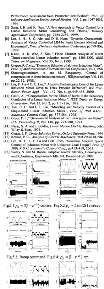
In this section, we make a series experiment on the adaptive controller design which is proposed in Section 3. For the exponential type of desired trajectory in Fig 5. I, we found chattering phenomenon in the steady state. In order to eliminate such phenomenon, we propose a PI control scheme while the position tracking error is kept within k100pm

.

After that, such arrangement will truly render the error less than

k l p m

.

In Fig 5.2, we adopt sinusoidal trajectories, the steady error is within

f0.5”

.

In Fig 5.3, we adopt a ramp command to relax the contraction smooth trajectory on experiment. It was also can achieve the position convergence. However, all the estimated parameters are truly bounded in this position tracking case.

5.2 Results of Adaptive Backsteeping controller for position tracking

For the position tracking problem, we provide several kinds of desired position trajectories, For the exponential trajectories in Fig 5.4, we found chattering phenomenon in the steady state error within

+50pm

. In Fig 5.5, we adopt sinusoidal trajectories, the steady error is within

k0.7”.

In Fig 5.6, we adopt a ramp command to relax the contraction of smooth trajectory on experiment.

VI.

CoNCLUSION

In this paper, we have proposed an adaptive position controller and an adaptation backstepping controller for the LIM with fifthkixth order nonlinear dynamic model which is control by the primary voltage source. To cope with the uncertainty part of the LIM, i.e., end effect, payload, and inductance, we design our controller based on an appropriate nonlinear transformation. Due to inaccessibility to the flux in general Stability analysis based on Lyapunov theory is performed to guarantee the controller design is stable. Finally, both the simulation and experimental results confirm the effectiveness of our control design.

Acknowledgement

R.O.C., under the grant NSC-89-2623-7-002- 004.

This research is sponsored by National Science Council,

Reference:

Yamamura, S . , Theory of Linear Induction Motors, John Wiley &

Sons, 1972.

Takahash 1. and Y. Ide, “Decoupling Control of thrust and attractive force of a LIM using a space vect or control inverter”, IEEE Trans on

Industry Applications, Vol. 29, pp. 161-167, 1993

Dolinar, D., G. Stumberger and B. Grcar, “Calculation of the Linear Induction Motor Model Parameters using Finite Elements”, IEEE

Trans. on Magndics, Vol. 34, No.5, pp.3640-3643, 1998.

Zhang, Z., Tony R. Eastham and G. E. Dawson “LlM Dynamic

Performance Assessment from Parameter Identification”, Porc. of

Indusby Application Society AnnualMeeting, Vol. 2, pp. 1047- 105 I, 1993.

Sung, J. H. and K. N q “A New Approach to Vector Control for a Linear Induction Ivbtor iconsidering End Effects,” Industry

Application Conference, pp. 2284-2289, 1999.

Lee, J. H., S . C. Ahn and D. S . Hyun “Dynamic Characteristic Analysis of Vector Controlled LIM by Finite Element Method and Experimed‘, Proc. oflndustty Applications Conference, pp.799 -806, 1998.

Kwon, B., K. Woo, S . Kim. “ Finite Element Analysis of Direct

Thrust-controlled Linear induction motor”, pp, 1306- 1309, IEEE

Trans. on Magnetics, Vol. 35, No.3, 1999.

Creppe, R.C. etc., “Dynamic Behavior of alinearhduction Motor”,

Proc. of Medifterranean Electrotechnical Conference, Vo. 2,1998.

Shanmugasundaram, A. and M. Rangasamy, “Control of compensation in linear induction motors”, IEEproceedingq Vol. 135, pp.22-32, 1988.

Lin, F. J. and C. C. Lee,“ Adaptive Backstepping Control for Linear Induction Motor Drive to Track Periodic Reference”, IEE Proc.

Electr. Power Appl.

Gastli, A., “Compensation for the Effect of Joints in the Secondary Conductor of a Linear Induction Motor”, IEEE Trans. on Energv Conversion,Vol. 13,No.2,pp.111-116, 1998.

Tsai, C. C. and C. L. Lai, “Modeling and Velocity Control of a Singlosided Linear lnducf ion Motor”, Proc. of 1998 R.O.C.

Automatic Control Conf, I)P. 577-584. 1998.

Vol. 147, No. 6, pp.449-458, 2000.

[ 131 Groot, D. J.,” Dimensional ikalysis of the Linear induction Motor”,

[ 141 Nasar, S. A. and 1. Boldea, Linear Motion Electric Machines, John

[ I51 GieraS J. F., Linearhduction Drives, OxfordUnivmity Press, 1994.

[ 161 Krause, P. C., Analysis of Electric Machinery, McGrrawHiU, 1986.

[ 171 Lee, H. T., L. C. Fu and Cola. Chen, “Nonlinear Adaptive Speed

Control of Induction Motor with Unknown Load Torque”, Proc. of 2001 R.O.C. Automatic Control ConJ, pp413-418, 2001.

[ 181 Sastry, S . and M. Bodon, Adaptive control: Stability, Convergence, and Robustness, Englewood cliffs. NJ: Prentice-Hall.1989.

IEE Proceeding-B, Vol. 140, pp. 273-280, 1993. Wiley & Sons, 1976.

m,

r,i

Irr ”11

Fig5.1 pd = 5(1 -e-*‘) c d s e c Fig5.2 pd = 5sin(2t) cm/sec

* A

” I ;

“ l r 3 %-air w,ir

Fig 5.3: Ramp command Fig 6.4: pd = (l-e-2‘) cm

l.zv-

, . . ...

. , * I....