Adaptive Asymptotic Bayesian Equalization Using a
Signal Space Partitioning Technique
Ren-Jr Chen and Wen-Rong Wu, Member, IEEE
Abstract—The Bayesian solution is known to be optimal
for symbol-by-symbol equalizers; however, its computational complexity is usually very high. The signal space partitioning technique has been proposed to reduce complexity. It was shown that the decision boundary of the equalizer consists of a set of hyperplanes. The disadvantage of existing approaches is that the number of hyperplanes cannot be controlled. In addition, a state-search process, that is not efficient for time-varying channels, is required to find these hyperplanes. In this paper, we propose a new algorithm to remedy these problems. We propose an approximate Bayesian criterion that allows the number of hyperplanes to be arbitrarily set. As a consequence, a tradeoff can be made between performance and computational complexity. In many cases, the resulting performance loss is small, whereas the computational complexity reduction can be large. The proposed equalizer consists of a set of parallel linear discriminant functions and a maximum operation. An adaptive method using stochastic gradient descent has been developed to identify the functions. The proposed algorithm is thus inherently applicable to time-varying channels. The computational complexity of this adaptive algo-rithm is low and suitable for real-world implementation.
Index Terms—Adaptive, Bayesian, nonlinear equalizer.
I. INTRODUCTION
E
QUALIZERS are commonly used in digital communica-tion systems to compensate for the channel effect. These equalizers can be classified as linear or nonlinear. In general, nonlinear equalizers may perform better, but their compu-tational complexity is higher. One exception is the decision feedback equalizer (DFE). The DFE is a nonlinear equalizer, but its computational complexity is low. In many applications, the linear equalizer or the DFE cannot give satisfactory results, and a more sophisticated nonlinear equalizer is required [22], [23]. Two kinds of nonlinear equalizers are well known: sequence estimation and symbol-by-symbol equalizers. The optimal sequence estimation equalizer is known to be the max-imum likelihood sequence estimation (MLSE) [1], whereas the optimal symbol-by-symbol equalizer is the Bayesian equalizer [2]. Although the MLSE yields the lowest bit error rate, its processing delay is larger, and its channel tracking ability is lower making it less effective for time-varying channels [24]. In this paper, we concentrate on the symbol-by-symbol equalizer.Although the Bayesian equalizer is optimal, its computational complexity is significantly higher than that of linear equalizers.
Manuscript received June 25, 2002; revised May 19, 2003. The associate ed-itor coordinating the review of this manuscript and approving it for publication was Dr. Naofal Al-Dhahir.
The authors are with the Department of Communication Engineering, National Chiao Tung University, Hsinchu 300, Taiwan, R.O.C. (E-mail: rzchen.cm88g@nctu.edu.tw; wrwu@cc.nctu.edu.tw).
Digital Object Identifier 10.1109/TSP.2004.826162
Thus, many nonlinear algorithms have been employed to ap-proximate or realize the Bayesian solution. In general, the struc-tures of these algorithms allow a tradeoff between performance and computational complexity. These algorithms include the polynomial-based nonlinear equalizer [3], [4] and the artificial neural network [5]–[12]. The disadvantages of these approaches are long training times and lack of methodologies for archi-tecture selection. In addition, their computational complexities may still be too high for many applications. Efficient algorithms for solving the Bayesian equalization problem were then devel-oped. The support vector machine (SVM) approach [13], [14], which is a nonlinear modeling tool, was applied to nonlinear equalization. It was shown that the computational complexity of the SVM can be much lower than polynomial and neural net-work-based equalizers. However, the learning algorithm in the SVM needs to solve a quadratic programming problem. The op-timization method is somewhat computationally intensive.
The other type of efficient algorithm employs the signal space partitioning technique [15]–[18]. This type of approach treats equalization as a classification problem. It has been shown that the Bayesian decision boundary consists of a set of hyperplanes when the signal-to-noise ratio (SNR) is infinite [17]. In [15] and [16],the authors used a combinatorial search and optimiza-tion process to find these planes. Despite its high computaoptimiza-tional complexity, this method is not guaranteed to obtain the asymp-totic Bayesian solution. It has been shown [17] that the hyper-planes can be formed by so-called dominant signal state pairs. A simpler method was proposed in [17] to search for these dom-inant pairs. This design is guaranteed to asymptotically achieve the Bayesian solution. The signal space partitioning techniques mentioned above all require channel information for signal state calculation. The number of hyperplanes and dominant states also depends on channel characteristics. If the channel response changes, the hyperplanes must be recalculated. Thus, these ap-proaches are inefficient for time-varying channels. An alternate method proposed in [25] partitions the signal space into several subspaces using the value of a received signal symbol. A hyper-plane is then used for the decision boundary in each subspace. The problem with this approach is that the decision boundary in each subspace may not be well approximated using a single hyperplane.
In this paper, we propose a new method that provides efficient approximation of the Bayesian solution. As in [15]–[18], we use a set of hyperplanes to form the decision boundary; however, the implication of these planes and the method for finding them are quite different. In existing methods, the number of hyper-planes is determined by channel responses. In our approach, the number of hyperplanes is arbitrarily set. The hyperplanes found
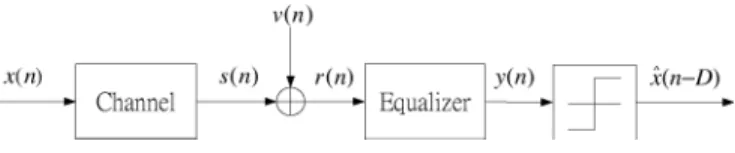
Fig. 1. Typical digital communication system.
by the proposed algorithm are generally different from those found by the method in [15]–[18]. Our method allows an easy tradeoff between complexity and performance. In many cases, we can make the performance loss small, whereas the compu-tational complexity reduction is large. Another feature is that the parameters of these hyperplanes can be adaptively identified using a stochastic gradient descent method. As a result, the pro-posed equalizer can be effectively applied to time-varying chan-nels. Signal detection is performed using a set of parallel linear discriminant functions followed by a maximum operation. The computational complexity of the proposed equalizer is low and suitable for real-world implementation.
This paper is organized as follows. Section II describes the symbol-by-symbol and optimum Bayesian equalizers. Section III discusses the concept and algorithm of the proposed equalizer. Section IV shows simulation results that demonstrate the effectiveness of the proposed equalizer. Section V gives some concluding remarks.
II. PROBLEMSTATEMENT
A typical digital communications system is shown in Fig. 1, where denotes the transmitted symbol, the channel output, the channel noise, the received signal, the equalizer output, and the equalizer output deci-sion where is the desired output delay. Let be the memory length of the channel,
be the channel input vector, and the channel input and output be characterized by a mapping function . We then have the following relationship:
(1) To simplify the problem, we assume that is a binary phase shift keying (BPSK) signal, i.e., , and is an additive white Gaussian noise (AWGN) with variance . Con-ventionally, equalization is treated as an estimation problem, and the output of the equalizer is viewed as an estimate of
. Let the memory length of the equalizer be ,
be the equalizer input vector, and the relationship between the equalizer input and output be described by a mapping function . A criterion is then optimized to find the unknown function. The minimum mean-square error (MMSE) criterion expressed as
is a commonly used one. Once the optimal function has been found, say, , the equalizer output may
be , and the decision if
and if . Finding the optimal
function may not be always desirable. A simpler approach is to use a predetermined function with unknown parameters and minimize the same criterion to find the parameters.
There is yet another way to solve the equalization problem.
Let and
. From (1), we have (2) If noise is absent, the equalizer output is then . From Fig. 1, we know that the memory size for the whole system
is . Thus, we have
(3) where
and denotes a vector mapping function. Since has two possible values 1 or 1, has , which is
possible combinations. From (3), we see that also has possible combinations. We call the signal vector and its possible values signal states. In practice, noise is always present. From (2), we see that will form clusters in a -dimen-sion Euclidean space. Thus, if we can classify the space into two subspaces corresponding to or 1 and de-termine to which subspace a given belongs, we solve the equalization problem. Thus, channel equalization can be viewed as a classification problem [7]. Denote as the signal state, , as the -dimension Euclidean space, and the set of all possible signal states in the space as
(4) We call the signal state set. Two subsets of are defined as
(5) The equalizer is then used to classify the received signal space (in ) into two regions and assign each region a decision value. This can be formulated as the hypothesis testing problem described as follows:
(6) (7) where is a discrete random vector, and its possible values are in . The optimum decision rule for this hypothesis testing problem is the Bayesian decision rule minimizing the proba-bility of error, i.e.,
(8)
Under the AWGN assumption, it was shown in [7] that the Bayesian decision rule is
where
(10)
III. PROPOSEDEQUALIZER
A. Approximate Bayesian Criterion
Although the Bayesian solution is optimal (in the minimum error probability sense), the computational complexity is usu-ally very high because in (10), there are exponential terms to be evaluated, and grows exponentially with . In this section, we propose a new method for solving this problem. Our idea is to reduce the number of terms involved in (10). First, we approximate (9) and (10) using the following decision rule: (11)
(12) Because the exponential operation is a monotonic function, the second equality in (12) holds. Due to the rapid-decay property of the Gaussian function, the decision using (11) and (12) usu-ally provides a good approximation to that using (9) and (10). It is straightforward to see that the smaller the noise level, the smaller the approximation error. The decision using (11) and (12) is asymptotically identical to that using (9) and (10). It is simple to show that the decision boundary of (11) always consists of hy-perplanes regardless of noise variance. The advantage of using (11) and (12) is that we do not have to evaluate exponential func-tions. However, we still have inner product terms to evaluate. To reduce computation, we divide (as well as ) into some subsets and merge states in each subset into a new state. If we let the number of all subsets be , we then have new states.
How to determine these new states optimally becomes the key problem. As we show below, the optimal new states are usually not in the signal space. For this reason, we call them pseudo states. Denote the set consisting of the pseudo states as
. We can then further approximate (12) as
(13) We now have inner product terms to evaluate instead of . If is significantly smaller than and equalizer performance is not affected, then the goal of complexity reduction has been achieved. As [17] showed, the Bayesian decision boundary con-sists of a set of hyperplanes if noise is absent. Each hyperplane is determined by a dominant state pair (a state in and an-other state in ). Only those terms associated with the dom-inant states need be evaluated. The number of domdom-inant pairs, however, is determined by the channel response. Although our
approach also leads to a decision boundary consisting of hyper-planes, there are some fundamental differences to the method in [17]. First, the number of pseudo states can be set arbitrarily in our approach and is not dependent on channels. We can then easily trade performance for complexity. Second, the pseudo states are found through minimization of some criterion and not by searching in space. Thus, the stochastic gradient method can be applied, and this results in an adaptive equalization al-gorithm. Note that hyperplanes found by the method in (13) are generally not identical to those by the method in [17]. The key problem is, as mentioned above, how to find those pseudo states. As we will show, our method is simple and effective.
B. Equalization Using a Single Hyperplane
We start with a simple case in which the number of pseudo states is two (i.e., one for and the other for ). From (13), we can see that the decision boundary is just a hyperplane. We propose using the following MMSE criterion and nonlinear function to estimate the pseudo states:
(14) where
(15)
where and denote the pseudo states. Derivation of the nonlinear function in (15) is shown in the Appendix. Equation (15) corresponds to the MMSE estimate of when the number of signal states are two and their values are known. Thus, we can say that if the number of signal states is actually two, the solution of (14) will give the true signal states. In gen-eral cases, the number of states in is greater than two. How do we interpret the equalization results using the pseudo state found in (14) and (15) and the decision rule in (13)? To answer this question, we first rewrite (14) as follows. If is 1, the resultant signal state is in , and the corresponding pseudo state is . On the contrary, if is 1, the re-sultant signal state is in , and the corresponding pseudo state is . Then, (14) can be rewritten as
(16) where
(17)
, when is 1, and , when
is 1. Note that is the same as in (15). We introduce this notation for later development convenience. From (16) and (17), we can observe that the form of the cost function is similar for both transmitted symbols. Only the output definition is different. If the signal state for a transmitted symbol is in and the received signal is closer to than , using the decision rule (13), we find that the decision is 1 and that it is correct. However, if is closer to than , the decision
is 1, and it is wrong. Note that if is small, the nonlinear function in (17) approaches a step function. When the decision is correct, the cost function tends to be 0. When the decision is wrong, the cost function tends to be a constant 4. The result is similar for the case in which the transmitted symbol signal state is in . This property has a significant implication, as described below.
A standard technique for classification employs a set of dis-criminant functions. A disdis-criminant function is designed to have a maximum value for a certain class of objects. As [26] reveals, a classifier using a discriminant function will yield a minimum classification error probability if the parameters of the function is obtained by minimizing a cost function that gives 0 value when the decision is right and a constant when the decision is wrong. As described above, we treat equalization as a classifica-tion problem. Two funcclassifica-tions in (13) actually correspond to two discriminant functions. Thus, we conclude that equalization re-sults using the decision rule in (13), and the associated pseudo state estimates found in (14) and (15) will achieve a minimum error probability.
Since (14) is highly nonlinear, it is difficult to obtain the so-lution directly. Here, we employ the adaptive method to solve the problem. There are at least two advantages to this approach. First, the optimal solution can be found using a process called training, and the computational complexity of the training al-gorithm is usually very low. Second, the equalizer can be con-tinuously trained using former decisions such that it can op-erate in a time-varying environment. The specific method we use is called the steepest descent method [27]. Let ,
and . For equations shown below, if the signal state for a training symbol is in , then . Otherwise, . Using the chain rule, we can have the gradient vectors from (16). Then, the update equations are given as
(18) (19) where is the step size. As we can see, the computational com-plexity requirement for the adaptive algorithm is quite low. Once the pseudo states are obtained, we can have as
(20) The decision is then
. (21)
From the stand point of classification, (20) and (21) divides re-ceived signal space into two regions and and as-signs a decision value to each region. We call the decision region for . From (20), we can have the decision region as
(22) (23)
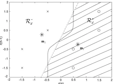
Fig. 2. Decision boundaries for the proposed (dashed line) and the Bayesian (solid line) equalizer with two subsets.
where
(24) (25) We now use an example to describe the algorithm proposed above.
Example 1: Consider a linear channel with memory length
and impulse response {1,0.5}. Since the channel is linear, the output is obtained using a convolution of and the channel response. Let and . Thus,
, and eight signal states result. The signal state set is then divided into two subsets corresponding to
and .
(26) The noise variance is set to 0.05. The proposed algorithm is applied to carry out equalization, and the result is shown in Fig. 2 in which the symbol “o” denotes the signal state corresponding to , and “x” denotes the signal state corresponding to . Since , the received signal space is a plane, and the decision boundary is a one-dimensional curve. As we can see from the figure, the decision boundary of the proposed algorithm is linear, which was expected. It is also interesting to note that the determined pseudo state in (or ) is quite close to one of the states in (or ). From the figure, it is apparent that there is much room for performance enhancement. If we can break the decision boundary into smaller pieces and approximate each piece using a linear boundary, we can better approximate the optimal decision boundary. To implement this idea, we must then subdivide (or ) into smaller subsets. This is elaborated upon in the next subsection.
C. Equalization Using Multiple Hyperplanes
In the previous subsection, we developed an equalization al-gorithm using a single hyperplane. The signal state set was divided into two subsets corresponding to , and two pseudo states were used. In this subsection, we extend this method to accommodate the general equalization problem. The idea is to subdivide each signal state set into more sub-sets. Each subset is represented by a pseudo state. A hyperplane decision boundary is then determined using a pair of pseudo states. Our subdividing approach is simple and straightforward. For example, the signal state set can be divided into four
sub-sets corresponding to and or
one corresponding to and .
To have a general formulation, we first rewrite the input vector as a combination of three vectors.
(27) where
(28)
where , and . Note
that includes , and its length is .
Depending on the value of , or may or may
not exist. For example, if , we do not have . Let . We then have possible vector values for . Denote these vectors as , . Now, we can divide the signal state set according to the value of : (29) and
(30)
For example, if we let , , and , then
, and the corresponding subsets are
(31) (32) (33) (34) If , we then have two signal subsets, and this de-generates to the case discussed above. We then define pseudo states to represent the corresponding sub-sets. Thus, we have decision regions associated with these subsets. For the time being, we assume that these pseudo states are known. The decision rule using (13) suggests that we can assign a received signal vector to subset if the distance to is minimal. Once the signal subset has been determined, the
Fig. 3. Structure of the proposed nonlinear equalizer.
value corresponding to the subset gives the decision. Define as a set with indexes such that
(35)
where is a vector, and
(36) In addition, define
(37) Thus, the output decision can be obtained as
(38)
. (39)
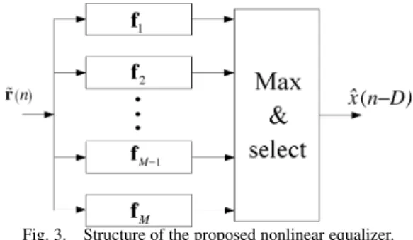
The overall structure of the proposed nonlinear equalizer is shown in Fig. 3. The response of each linear discriminant
function in Fig. 3 corresponds to , and
the input of each function is . If is in
the decision region of subset , then
and
(40) Note that each inequality in (40) forms a hyperplane between Subset and . If we pretend that only these two subsets exist, this gives a decision region for subset . For the same subset ,
there are such regions , and
the true decision region for subset is the intersection of these regions. Let be the decision region formed by subset and (with respect to subset ), and is the decision region for subset . Then
(41) and
(42) Then, the final decision region corresponding to
is
(43) To have a better understanding of this idea, we give an example here.
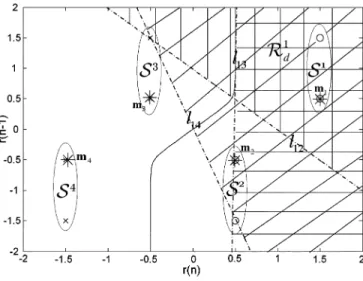
Fig. 4. Decision region of subset 1,R .
Example 2: Consider the same scenario given in Example 1.
We divide signal state set into four subsets using the method described in (31)–(34). This means that
, where and
. Note that is absent in this case. We then have the corresponding subsets
(44)
(45)
(46)
(47) The proposed algorithm is then applied to perform equalization. Fig. 4 shows how a decision region is formed in detail. Here, we use for detailed description. Since , the region is formed by three dashed lines , , and , where is the decision boundary between and . It is obtained by
solving , 2, 3, and 4. Symbol in the
figure represents pseudo states. The three shadow regions on the
right side of show the region of . We
can see that shadow region is the intersection of all regions
for , 2, 3, and 4. Fig. 5 shows all
of the decision regions , 1, 2, 3, and 4. By definition
in (35), , and . The decision
corresponding to is then
(48) (49) The final decision boundary can also be seen in Fig. 5. It shows that the decision boundary of the proposed equalizer is very close to that of the Bayesian equalizer. However, as we show below, the computational complexity of the proposed algorithm is significantly lower.
Fig. 5. Decision regions for all subsetsR i = 1; 2; 3; 4 and decision boundaries of the proposed (dashed line) and the Bayesian (solid line) equalizer.
We next describe how to find the pseudo states . We extend the method in (16). If the signal state for a transmitted symbol is in , then the cost function to be minimized is defined as
(50) where
(51) Note that tends to be 0 if the decision is right and a value less than if the decision is wrong. Thus, as mentioned above, the decision rule associated with the estimates in (51) will yield a minimum error probability among all detectors using the same number of hyperplanes. To find the pseudo states, we still apply the adaptive method. For each received signal vector , we can obtain its corresponding signal state . According to , we know to which subset the signal state belongs (in training mode). The stochastic gradient descent method can still be used here. We then perform pseudo state adaptation similar to (18) and (19). If a received signal vector belongs to subset , we then have the following adaptive
algorithm :
(52)
(53)
Note that the physical interpretation of the value 1 in (52) and (53) is different from that in (18) and (19). In (18) and (19), the value of 1 corresponds to the desired signal, which is , whereas in (52) and (53), it is just a desired constant for a right decision.
Since the cost function is a nonlinear function, the adaptive algorithm may converge to a local minimum. Thus, the proper choice of initial value is important. We suggest using the clus-tering method [11] to obtain a reliable initial value. The compu-tational complexity requirement for this algorithm is very low. The clustering method is given as
if
counter counter counter
counter
end. (55)
We have thus assumed that the noise variance is known a
priori. As a matter of fact, this assumption is not required. The
smaller the noise variance, the more closely the function in (54) approaches a step function, and the closer the equalizer is to achieve the optimal performance (minimum classification rate). However, the adaptive algorithm also converges more slowly, which affects the final pseudo states positions. Thus, we can treat as a design parameter. As we show in the next section, the equalization results are not sensitive to the choice of this parameter. Denote the parameter as . According to the adaptive algorithm given above, we may summarize the overall adaptive algorithm to adjust as follows:
1) Initially set by the
clustering method
2) For each instant of time, ,
if
for and
end end
The proposed method described above partitions the signal space into subsets, where is an integer. It is straightforward to relax this constraint and partition the signal space into an arbitrary number of subsets. The details, however, are omitted here.
With a minor modification, the clustering algorithm described above can find the mean of each cluster as well as the vari-ance. Assuming that each cluster has a Gaussian distribution and treating its mean as a state, we can then apply the Bayesian deci-sion rule. We call this a reduced-state (RS) Bayesian equalizer.
TABLE I
COMPUTATIONALCOMPLEXITYCOMPARISON FOR THELINEAR ANDPROPOSED
EQUALIZERS IN THETRAININGPHASE
TABLE II
COMPUTATIONALCOMPLEXITYCOMPARISON FOR THELINEAR, PROPOSED,
ANDBAYESIANEQUALIZERS IN THEDECISIONPHASE
Depending on the number of clusters, the computational com-plexity of the RS Bayesian equalizer can be much lower than that of the original Bayesian equalizer. However, as we show in the next section, the performance of the RS Bayesian equalizer is poor unless the number of the clusters is large.
D. Computational Complexity
There are two phases for the proposed algorithm: the training and decision phases. For simplicity, we treat the computational requirement for division the same as that for multiplication. We summarize the overall computational requirement for both phases in Tables I and II. Roughly speaking, in the decision phase, the complexity of the proposed equalizer is times higher than the linear equalizer. The actual choice of is de-pendent on the desired performance. In our design, the decision region for each subset is automatically and adaptively formed, and these decision regions are approximations of Bayesian de-cision regions. In principle, if the Bayesian dede-cision boundary has a complex shape, we need more subsets. In many cases, however, only a small number of subsets is sufficient. The com-putational complexity of the proposed equalizer can be much lower than that of the Bayesian equalizer because can be much smaller than without significantly sacrificing perfor-mance. Note that if a time-varying channel is considered, deci-sions can be used to train the proposed equalizer continuously such that channel variations can be properly tracked. In this case, the computational complexity for the proposed equalizer is the summation of that listed in Table I (the adaptive part) and that in Table II. Since the value of used is usually small, the overall complexity will not be increased significantly.
IV. SIMULATIONRESULTS
In this section, we report simulation results demonstrating the effectiveness of the proposed equalizer. Two linear channels and one nonlinear channel were used. We compared the proposed equalizer with an optimum Bayesian equalizer, a conventional MMSE linear equalizer, and a minimum bit error rate (MBER) linear equalizer [20]. To reflect the relative noise level, we de-fined the SNR as the ratio of and , where is the variance
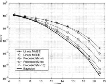
Fig. 6. BER comparison for the MMSE linear, MBER linear, proposed, and Bayesian equalizers.
of , and is that of . The bit error rate (BER) was used as the performance measure. We first considered a linear channel [11]. The channel is described using a difference equa-tion as
(56) As we can see, the channel length is 3 . For all
equal-izers compared, we let and . Thus,
. For the proposed equalizer, we let
and , for which and
, respectively. The sim-ulation results for various SNR conditions are shown in Fig. 6. In the figure, we see that the performance of the MMSE linear equalizer was the worst, and the Bayesian one was the best. There is a performance gap between them. The performance of the linear MBER equalizer [20], [21] was only slightly better than that of the linear MMSE equalizer. The performance of the proposed equalizer was close to that of the Bayesian equal-izer when . However, the computational complexity was significantly lower. While the performance of the proposed equalizer when was worse than when , it was much better than that of the MBER linear equalizer. We ob-served the learning curve for the proposed equalizer ( and SNR dB) and found that the adaptive algorithm converged around 5000 iterations. Fig. 7 gives a performance comparison for the proposed and the RS Bayesian equalizers. The RS Baysian equalizer performed poorly when and . Although the performance of the RS Bayesian equalizer was good when , it was worse than that of the proposed equalizer when . We have also tried various values for the proposed algorithm . We varied from 0.05 to 0.8 and found that the performance was almost unaffected. The pro-posed algorithm performance is not sensitive to the choice of . The second channel we considered was also a linear channel [7]:
(57)
Fig. 7. BER comparison for the proposed and RS Bayesian equalizers.
Fig. 8. BER comparison for the MMSE linear, MBER linear, proposed and Bayesian equalizers.
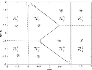
We let and for all equalizers. Note that for this scenario, the signal state spaces and were not lin-early separable. Since , . We also used and for the proposed equalizer. The simulation results are shown in Fig. 8. In the figure, we can see that the perfor-mance of the linear equalizers was very poor. This is not sur-prising since the signal space was not linearly separable. Even for high SNRs, the linear equalizers could not give satisfactory results. Nonlinear equalizers are not affected by this problem: The higher the SNR, the lower the BER. The performance of the proposed equalizer was very close to that of the Bayesian equal-izer. When , there was almost no difference. To explain this, we show decision boundaries for the Bayesian equalizer and the proposed equalizer when in Fig. 9. In the figure, we can clearly see that the decision boundary of the proposed equalizer closely approximated that of the Bayesian equalizer. Only in the central region in Fig. 9 is there some discrepancy. However, this does not contribute significant bit errors. The de-cision boundary for the proposed equalizer when is fur-ther shown in Fig. 10. Note that the decision boundary of the
Fig. 9. Decision regions for all subsetsR i = 1; 2; 3; 4 and decision boundaries of the proposed equalizer whenM = 4 (dashed line) and the Bayesian (solid line) equalizer.
Fig. 10. Decision regions for all subsetsR i = 1; 2; 1 1 1 ; 8 and the decision boundaries of the proposed equalizer whenM = 8 (dashed line) and the Bayesian (solid line) equalizer.
proposed equalizer almost exactly matched that of the Bayesian equalizer. Note also that the pseudo states identified were very close to the true signal states. This was expected since there was only one state in each subset. It is important to realize that even in this case, the computational complexity of the proposed al-gorithm was still lower than that of the Bayesian equalizer.
We next considered a nonlinear channel, which is a linear channel followed by a memoryless nonlinearity. The input–output relationship of the linear channel is given by
(58) The output of the memoryless nonlinearity is given by
(59) For this case, , and set and for the equal-izers. It turned out that . The number of states was
Fig. 11. BER comparison for the MMSE linear, MBER linear, proposed, and Bayesian equalizers.
TABLE III
COMPUTATIONALCOMPLEXITYCOMPARISON FOR THELINEAR, PROPOSED
(M = 8),ANDBAYESIANEQUALIZERS(FOR THENONLINEAR
CHANNEL INSIMULATIONS)
then large, and the computational complexity of the Bayesian equalizer became huge. Fig. 11 shows the performance for these equalizers. Each BER result was obtained using runs. As the figure shows, the nonlinear equalizers significantly outper-formed the linear ones. The proposed equalizer efficiently ap-proximated the optimal Bayesian equalizer. While the perfor-mance loss was moderate, the computational complexity re-duction was significant. Table III shows a computational com-plexity comparison for all equalizers (in the decision phase).
V. CONCLUSION
An adaptive nonlinear equalizer is proposed. This equalizer was derived using an approximate Bayesian criterion. It con-sists of a set of parallel linear discriminant functions followed by a maximum function. The number of functions can be arbi-trarily chosen, and the corresponding coefficients can be adap-tively trained. Thus, we can have the flexibility to trade perfor-mance for reduced computational complexity. We demonstrated that the proposed equalizer can closely approximate the perfor-mance of an optimal Bayesian equalizer, whereas its computa-tional complexity remains significantly lower. Due to its adap-tive nature, this equalizer is applicable to time-varying chan-nels. The adaptive algorithm with the stochastic gradient de-scent is simple and robust, which will be a great advantage for real-world applications.
The idea of subset partition can be further extended. For ex-ample, if we want to have eight subsets, we may choose
el-ements, we can partition the signal space into eight subsets. This is different from the partitioning method described in this paper, where all three elements of must be consecutive. The specific elements to choose may depend on the channel mapping function. An intuitive thought is to choose the ones contributing most energy in the received signal vector. To do that, we may need a channel identification filter. This extended method may make the signal subsets more linearly separable and facilitate decisionmaking.
APPENDIX
Consider an equalizer whose output is determined using the MMSE criterion described below.
(60)
The optimal solution for this cost function is known to be the conditional mean [19], which is
(61) For the equalization problem mentioned above, we have
(62) Let the number of elements in be one. Using the Bayes rule and the fact that
, we have
(63)
where is the a priori probability
den-sity function (PDF) conditioned on , and is the PDF of . They are given as follows:
(64)
(65)
where is the only state in , and is the only state in . Note that
(66)
Substituting (63)–(66) into (61) and (62) and simplifying the result, we obtain
(67)
REFERENCES
[1] G. D. Forney, “Maximum-likelihood sequence estimation of digital se-quences in the presence of intersymbol interference,” IEEE Trans.
In-form. Theory, vol. IT-18, pp. 363–378, Mar. 1972.
[2] S. Chen, S. McLaughlin, and B. Mulgrew, “Complex valued radial basis function network, Part II: Application to digital communications channel equalization,” Signal Process., vol. 35, no. 1, pp. 175–188, Jan. 1994.
[3] S. Chen, G. J. Gibson, and C. F. N. Cowan, “Adaptive channel equal-ization using a polynomial-perceptron structure,” Proc. IEE, pt. 1, vol. 137, no. 5, pp. 257–264, 1990.
[4] Z. Xiang, G. Bi, and T. Le-Ngoc, “Polynomial perceptrons and their applications to fading channel equalization and co-channel interference suppression,” IEEE Trans. Signal Processing, vol. 42, pp. 2470–2480, Sept. 1994.
[5] G. J. Gibson, S. Siu, and C. F. N. Cowan, “Application of multilayer perceptrons as adaptive channel equalisers,” in Proc. IEEE Int.
Conf. Acoust., Speech, Signal Processing, Glasgow, U.K., 1989, pp.
1183–1186.
[6] , “The application of nonlinear structures to the reconstruction of binary signals,” IEEE Trans. Signal Processing, vol. 39, pp. 1877–1884, Aug. 1991.
[7] S. Chen, G. J. Gibson, C. F. N. Cowan, and P. M. Grant, “Reconstruc-tion of binary signals using an adaptive radial-basis-func“Reconstruc-tion equalizer,”
Signal Process., vol. 22, pp. 77–93, 1991.
[8] I. Cha and S. A. Kassam, “Channel equalization using adaptive complex radial basis function networks,” IEEE J. Select. Areas Commun., vol. 13, pp. 122–131, Jan. 1995.
[9] J. Cid-Sueira, A. Artes-Rodriguez, and A. R. Figueiras-Vidal, “Recur-rent radial basis function networks for optimal symbol-by-symbol equal-ization,” Signal Process., vol. 40, pp. 53–63, 1994.
[10] S. Chen, S. McLaughlin, B. Mulgrew, and P. M. Grant, “Adaptive Bayesian decision feedback equaliser for dispersive mobile radio channels,” IEEE Trans. Commun., vol. 43, pp. 1937–1946, May 1995. [11] S. Chen, B. Mulgrew, and P. M. Grant, “A clustering techniques for
digital communications channel equalization using radial basis func-tion networks,” IEEE Trans. Neural Networks, vol. 4, pp. 570–579, July 1993.
[12] T. Adali, X. Liu, and M. K. Sönmez, “Conditional distribution learning with neural networks and its application to channel equalization,” IEEE
Trans. Signal Processing, vol. 45, pp. 1051–1064, Apr. 1997.
[13] D. J. Sebald and J. A. Bucklew, “Support vector machine techniques for nonlinear equalization,” IEEE Trans. Signal Processing, vol. 48, pp. 3217–3226, Nov. 2000.
[14] S. Chen, S. Gunn, and C. J. Harris, “Decision feedback equaliser design using support vector machines,” Proc. Inst. Elect. Eng. Vis. Image Signal
Process, vol. 147, no. 3, June 2000.
[15] Y. Kim and J. Moon, “Delay-constrained asymptotically optimal detec-tion using signal-space partidetec-tioning,” in Proc. IEEE ICC, Atlanta, GA, 1998.
[16] , “Multidimensional signal space partitioning using a minimal set of hyperplanes for detecting ISI-corrupted symbols,” IEEE Trans.
Commun., vol. 48, pp. 637–647, Apr. 2000.
[17] S. Chen, B. Mulgrew, and L. Hanzo, “Asymptotic Bayesian decision feedback equalizer using a set of hyperplanes,” IEEE Trans. Signal
Pro-cessing, vol. 48, pp. 3493–3500, Dec. 2000.
[18] S. Chen, L. Hanzo, and B. Mulgrew, “Decision feedback equalization using multiple-hyperplane partitioning for detecting ISI-corrupted M-ary PAM signals,” IEEE Trans. Commun., vol. 49, pp. 760–764, May 2001.
[19] H. V. Poor, An Introduction to Signal Detection and Estimation, 2nd ed. New York: Springer.
[20] C. C. Yeh and J. R. Barry, “Approximate minimum bit-error rate equal-ization for binary signaling,” in Proc. Int. Conf. Commun., vol. 2, Mon-treal, QC, Canada, June 1997, pp. 1095–1099.
[21] S. Chen, E. Chng, B. Mulgrew, and G. Gibson, “Minimum-BER linear-combiner DFE,” in Proc. IEEE Int. Contr. Conf., 1996, pp. 1173–1177. [22] S. Benedetto and E. Biglieri, “Nonlinear equalization of digital satellite channels,” IEEE J. Select. Areas Commun., vol. SAC-1, pp. 57–62, Jan. 1983.
[23] G. Karam and H. Sari, “Analysis of predistortion, equalization, and ISI cancellation techniques in digital radio systems with nonlinear transmit amplifiers,” IEEE Trans. Commun., vol. 37, pp. 1245–1253, Dec. 1989. [24] S. U. H. Qureshi, “Adaptive equalization,” Proc. IEEE, vol. 73, pp.
1349–1387, Sept. 1985.
[25] C. P. Callender, C. F. N. Cowan, and S. Theodoridis, “Non-linear adap-tive equalization using a switched coefficient adapadap-tive filter,” in Proc.
IEE Colloq. Adaptive Filtering, Nonlinear Dynamics Neural Networks,
1991, pp. 3/1–3/4.
[26] B. H. Juang and S. Katagiri, “Discriminative learning for minimum error classification,” IEEE Trans. Signal Processing, vol. 40, pp. 3043–3054, Dec. 1992.
[27] S. Haykin, Adaptive Filter Theory, 3rd ed. New York: Prentice-Hall, 1996.
Ren-Jr Chen was born in Taipei, Taiwan, R.O.C., in
May 1975. He received the B.E. degree in electrical engineering from Feng Chia University, Taichung, Taiwan, in 1997 and the M.S. degree in electrical engineering from National Tsing Hua University, Hsinchu, Taiwan, in 1999. Since 1999, he has been with the Department of Communication Engi-neering, National Chiao Tung University, Hsinchu, where he is currently pursuing the Ph.D. degree.
His research interests include communication signal processing, mainly adaptive nonlinear equalization.
Wen-Rong Wu (M’89) received the M.S. and Ph.D.
degrees in electrical engineering from State Univer-sity of New York at Buffalo in 1986 and 1989, respec-tively.
Since August 1989, he has been a faculty member with the Department of Communication Engineering, National Chiao Tung University, Hsinchu, Taiwan. R.O.C. His research interests include statistical signal processing and digital communications.