Efficient mining of generalized association rules with non-uniform minimum support

Efficient Mining of Generalized Association Rules with Non-uniform

Minimum Support

Ming-Cheng Tseng1and Wen-Yang Lin2,* 1

Institute of Information Engineering I-Shou University

Kaohsiung 840, Taiwan clark.tseng@msa.hinet.net 2

Department of Computer Science and Information Engineering National University of Kaohsiung

Kaohsiung 811, Taiwan wylin@nuk.edu.tw *

(Corresponding author)

Abstract. Mining generalized association rules between items in the presence of taxonomies has

been recognized as an important model in data mining. Earlier work on generalized association rules confined the minimum supports to be uniformly specified for all items or for items within the same taxonomy level. This constraint on minimum support would restrain an expert from discovering some deviations or exceptions that are more interesting but much less supported than general trends. In this paper, we extended the scope of mining generalized association rules in the presence of taxonomies to allow any form of user-specified multiple minimum supports. We discuss the problems of using classic Apriori itemset generation and presented two algorithms, MMS_Cumulate and MMS_Stratify, for discovering the generalized frequent itemsets. Empirical evaluation showed that these two algorithms are very effective and have good linear scale-up characteristics.

Keywords: Data mining, generalized association rules, multiple minimum supports, taxonomy.

1. Introduction

Mining association rules from a large business database, such as transaction records, has been an important topic in the area of data mining. This problem is motivated by applications known as market basket analysis to find relationships between items purchased by customers, that is, what kinds of products tend to be purchased together [1]. Such information is useful in many aspects of market management, such as store layout planning, target marketing, and understanding customer behavior.

An association rule is an expression of the form A B, where A and B are sets of items. Such a rule reveals that transactions in the database containing items in A tend to contain items in B, and the probability, measured as the fraction of transactions containing A also containing B, is called the

confidence of the rule. The support of the rule is the fraction of the transactions that contain all items

in both A and B.

For example, an association rule,

Desktop PC Ink-jet printer (sup = 30%, conf = 60%),

says that 30% (support) of customers purchase both Desktop PC and Ink-jet printer together, and 60% (confidence) of customers who purchase Desktop PC also purchase Ink-jet printer.

For an association rule to hold, the support and the confidence of the rule should satisfy a user-specified minimum support called minsup and minimum confidence called minconf, respectively. The problem of mining association rules is to discover all association rules that satisfy minsup and

minconf. This task is usually decomposed into two steps:

1. Frequent itemset generation: generate all itemsets that exceed the minsup.

2. Rule construction: construct all association rules that satisfy minconf from the frequent itemsets in Step 1.

Intuitively, to discover frequent itemsets, each transaction has to be inspected to generate the supports of all combinations of items, which, however, will suffer for lots of I/O operations as well as computations. Therefore, most early work was focused on deriving efficient algorithms for finding frequent itemsets [2][4][9][10]. The most well-known is Apriori [2], which relies on the observation that an itemset can be frequent if and only if all of its subsets are frequent and thus a level–wise inspection proceeding from frequent 1-itemsets to the maximal frequent itemset can avoid large numbers of I/O accesses.

Despite the great achievement in improving the efficiency of mining algorithms, the existing association rule models used in all of these studies incur some problems. First, in many applications, there are taxonomies (hierarchies), explicitly or implicitly, over the items. It may be more useful to find association at different levels of the taxonomy [5][11] than only at the primitive concept level.

Second, the frequencies of items are not uniform. Some items occur very frequently in the transactions while others rarely appear. A uniform minimum support assumption would hinder the discovery of some deviations or exceptions that are more interesting but much less supported than general trends. Furthermore, a single minimum support also ignores the fact that support requirement varies at different levels when mining association rules in the presence of taxonomy.

These observations lead us to the investigation of mining generalized association rules across different levels of taxonomy with non-uniform minimum supports. The methods we propose not only can discover associations that span different hierarchy levels but also have high potential in producing rare but informative item rules.

The remainder of this paper is organized as follows. The problem of mining generalized association rules with multiple minimum supports is formalized in Section 2. In Section 3, we explain the proposed algorithms for finding frequent itemsets. The evaluation of the proposed algorithms on IBM synthetic data and Microsoft foodmart2000 is described in Section 4. A review of related work is

given in Section 5. Finally, our conclusions are stated in Section 6.

2. Problem Statement

In this section, the basic concept behind generalized association rules in [11] is introduced. We then extend this model to incorporate multiple minimum supports.

2.1 Mining generalized association rules

Let I {i1, i2,…,im} be a set of items and D{t1, t2,…,tn} be a set of transactions, where each

transaction ti=tid, Ahas a unique identifier tid and a set of items A (A I). To study the mining of

generalized association rules from D, we assume that the taxonomy of items, T, is available and denoted as a directed acyclic graph on IJ, where J { j1, j2,…,jp} represents the set of generalized

items derived from I. An edge in T denotes an is-a relationship, that is, if there is an edge from j to i we call j a parent (generalization) of i and i a child of j. The meanings of ancestor and descendant follow from the transitive-closure of the is-a relationship. Figure 1 illustrates a taxonomy constructed for I = {Laser printer, Ink-jet printer, Dot matrix printer, Desktop PC, Notebook, Scanner} and J = {Non-impact printer, Printer, PC}.

Note that the above transactions and taxonomy definitions imply that all leaves in T are formed from I while others are from J but only real items in I can appear in the transactions.

Definition 1. Given a transaction ttid, A, we say an itemset B is in t if every item in B is in A or is

an ancestor of some items in A. An itemset B has support s, denoted as ssup(B), in the transaction set D if s% of transactions in D contain B.

Printer PC Scanner

Non-impact Dot-matrix Desktop Notebook

Laser Ink-jet

Fig. 1. An example of taxonomy.

Definition 2. Given a set of transactions D and a taxonomy T, a generalized association rule is an

implication of the following form

A B,

where A, BI J, A B , and no item in B is an ancestor of any item in A. The support of this rule, sup(A  B), is equal to the support of A B. The confidence of the rule, conf(A  B), is the ratio of sup(AB) versus sup(A), i.e., the fraction of transactions in D containing A that also contain

B.

According to the definition of generalized association rules, an itemset is composed not simply of items in leaves of the taxonomy but also of generalized items in higher levels of the hierarchy. This is why we must take the ancestors of items in a transaction into account while determining the support of an itemset. In addition, the condition in Definition 2 that no item in B is an ancestor of any item in A is essential; otherwise, a rule of the form, a ancestor(a), always has 100% confidence and is trivial. Definition 3. The problem of mining generalized association rules is that, given a set of transactions

D and a taxonomy T, find all generalized association rules that have support and confidence greater than a user-specified minimum support (minsup) and minimum confidence (minconf), respectively.

2.2 Multiple-support specification

To allow the user to specify different minimum supports for different items, we have to extend the uniform support used in generalized association rules. The definition of generalized association rules remains the same but the minimum support is changed. Following the concept in [7], we assume that the user can specify different minimum supports for different items in the taxonomy.

Definition 4. Let ms(a) denote the minimum support of an item a in IJ. An itemset A = {a1, a2,…,

ak}, where aiI J for 1 i k, is frequent if the support of A is larger than the lowest value of

minimum support of items in A, i.e.,

sup(A)

A a_i

min ms(ai),

Definition 5. A generalized association rule A  B is strong if the support satisfies the following

condition sup(A B)  B A ai min ms(ai), and conf(A B) minconf.

Definition 6. Given a set of transactions D, a taxonomy T composed of items a1, a2,…,an, and a

minimum confidence, minconf, the problem of mining generalized association rules with multiple user-specified minimum item supports ms(a1), ms(a2),…,ms(an) associated with each item in T is to

find all generalized association rules that are strong.

The idea of mining generalized association rules with multiple minimum supports is better illustrated with an example.

Example 1. Suppose that a shopping transaction database D in Table 1 consists of items I = {Laser

printer, Ink-jet printer, Dot matrix printer, Desktop PC, Notebook, Scanner} and the taxonomy T is as shown in Figure 1. Let the minimum support (ms) associated with each item in the taxonomy be as follows:

ms(Printer)80% ms(Non-impact)65% ms(Dot matrix)70% ms(Laser)25% ms(Ink-jet)60% ms(Scanner)15% ms(PC)35% ms(Desktop)25% ms(Notebook)25%

Let minconf be 60%. The support of the following generalized association rule,

PC, Laser Dot matrix (sup 16.7%, conf 50%),

is less than min{ms(PC), ms(Laser), ms(Dot matrix)} 25%, which makes this rule fail. However, another rule,

PC Laser (sup 33.3%, conf 66.7%),

holds because the support satisfies min{ms(PC), ms(Laser)}25%, and the confidence is larger than

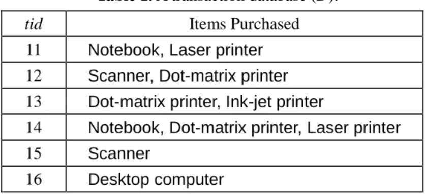
minconf . Table 2 lists the frequent itemsets and resulting strong rules.

Table 1. A transaction database (D).

tid Items Purchased

11 Notebook, Laser printer 12 Scanner, Dot-matrix printer 13 Dot-matrix printer, Ink-jet printer

14 Notebook, Dot-matrix printer, Laser printer

15 Scanner

16 Desktop computer

One of the difficulties in applying association rules mining to real-world applications is the setting of support constraint. The situation becomes worse when non-uniform, multiple item support specifications are allowed. The simplest method is to leave the work to the users. This approach has the most flexibility but places the users in a dilemma: How to specify the most appropriate support constraint, either uniform or non-uniform, to discover interesting patterns without suffering from combinatorial explosion and missing some less-supported but perceptive rules.

A more instructive method is using the frequencies (or supports) of items within the database [7], defined as follows: ms(a)       otherwise ) ( if , ), ( sup a minsup minsup a sup   (1)

where the parameter (0 1) is employed to control how the minimum support of an item a,

ms(a), is related to its actual frequency in the database. If 0, the specification degenerates to the

uniform case. As the formula indicates, users still have to specify the value of minsup and an additional parameter. The problem thus remains tangling.

Table 2. Frequent itemsets and association rules generated for Example 1.

Itemset min ms (%) Support (%)

{Scanner} 15 33.3

{PC} 35 50.0

{Notebook} 25 33.3

{Laser} 25 33.3

{Scanner, Printer} 15 16.7

{Scanner, Dot matrix} 15 16.7

{Laser, PC} 25 33.3

{Notebook, Printer} 25 33.3

{Notebook, Non-impact} 25 33.3

{Notebook, Laser} 25 33.3

Rules

PC Laser (sup 33.3%, conf 66.7%) Laser PC (sup 33.3%, conf 100%) Notebook Printer (sup 33.3%, conf 100%) Notebook Non-impact (sup 33.3%, conf 100%)

Notebook Laser (sup 33.3%, conf 100%) Laser Notebook (sup 33.3%, conf 100%)

To solve this problem, we have proposed in [6] an approach for minimum support specification without consulting users. The basic idea of our approach is to “push”the confidence and lift measure (or called positive correlation [3][8]) into the support constraint to prune the spurious frequent itemsets that fail to generate interesting associations as early as possible. First, let us show how the constraint is specified to reduce the frequent itemsets that fail in generating strong associations.

Lemma 1. Let AB be a frequent itemset, AB , and without loss of generality, let a A and a be

the one with the smallest minimum support, i.e., ms(a) 

B A ai

min ms(ai). If the minimum support of a is

set as ms(a)sup(a) × minconf, then the association rule A  B is strong, i.e., sup(AB) / sup(A)  minconf.

Proof. Since AB is frequent, sup(AB) ms(a) sup(a) × minconf. Furthermore, sup(a) sup(A)

According to Lemma 1, the minimum support of an item a, for aIJ, is specified as follows:

ms(a)sup(a) × minconf . (2)

Note that Lemma 1 does not imply that the rule B  A is strong. This is because the confidence measure is not symmetric over the antecedence and consequence. Therefore, Eq. 2 does not guarantee that all rules generated from the frequent itemsets will be strong.

Next we consider how to specify the constraint to generate interesting associations.

Definition 7. An association rule is interesting if it is strong and

lift(A B)  ) ( ) ( ) ( B sup A sup B A sup 

_

In the above definition, we have introduced an extra constraint, lift, which is employed to measure the deviation of the rule from correlation. For example, consider the transaction database in Table 1. For a minimum support of 30% and minimum confidence of 50%, the following association rule is discovered:

Scanner Printer (sup = 33.3%, conf = 50%).

One may conclude that this rule is interesting because of its high support and high confidence. However, note that the support of the generalized item Printer is 66.7%. This means that a customer who is known to purchase Scanner is less likely to buy Printer (by 16.7%) than a customer about whom we have no information. In other words, buying Scanner and purchasing Printer is negatively correlated, indicated by lift = 50/66.7 = 0.75 < 1.

Theorem 1. Let I be a set of items and the minimum support of each item be specified below

ms(ai) sup(ai) × } {

max

Then any strong association rule A B, for A, BI and AB, is interesting.

Proof. Since A B is strong, sup(AB) 

B A

amin ms(a). Specifically, let aai.Then, we have

sup(AB) ms(ai)sup(ai) ×

} { max i j I J a a  sup(aj).

Since AB , aibelongs to either A or B. Without loss of generality, let aiA. It is easy to show

that

sup(A)sup(ai) and sup(B)

} { max i j I J a a  sup(aj).

The lemma then follows. ■

Note that the support constraint specified in Eq. 3 only provides a sufficient condition for obtaining interesting association rules from frequent itemsets. There may exist some itemsets that are infrequent with respect to this constraint but can generate positive lift associations. To construct all associations without missing any positive lift rule, we should refine the support specification. The intuition is to set the minimum support of an item a to accommodate all frequent itemsets that consist of a as the smallest supported item and are capable of generating at least one positive lift association rule.

Without loss of generality, we assume that a A and a is the one with the smallest minimum support over itemset A B, i.e., ms(a) 

B A

a_imin ms(a i), and bB, ms(b) aiB

min ms(ai). The following

conditions hold,

sup(AB) ms(a), sup(A) sup(a), and sup(B) sup(b).

Thus, to make lift(A B) 1, we would specify ms(a) sup(a) sup(b). Note that b can be any item in the item set I except a, and sup(b) sup(a). What we need is the smallest qualified item, i.e., b  min{ai| aiI {a} and sup(ai)sup(a)}. Let I {a1, a2, ..., an}, and sup(ai)sup(ai+1), 1i n 1.

The minimum item support with respect to nonnegative lift can be specified as follows:

ms(ai)          _ n i n i a sup a sup a sup i i i if 1 1 if ), ( ), ( ) ( 1 (4)

Now we have two separate support settings: The first is based on the confidence measure and the second is based on lift. To prune the spurious frequent itemsets so as to make most of the generated rules become interesting, we combine these two specifications as shown below, which we call the

confidence-lift support constraint (CLS). ms(ai)          _ n i n i a sup a sup minconf a sup i i i if 1 1 if ), ( )}, ( , max{ ) ( ₁ (5)

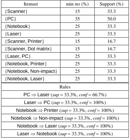
Example 2. Let minconf 50%. The first two columns of Table 3 show the sorted list of all items,

primitive or generalized, along with their supports. Then, according to Eq. 5, it is not hard to derive the minimum item supports, as shown in the last column. For example, ms(Desktop) sup(Desktop)  max{minconf, sup(Ink-jet)} = 1/6 1/2 8.3%, ms(PC) sup(PC) max{minconf, sup(Printer)} = 1/22/3 33.3%, and ms(Printer) sup(Printer) 66.7% since Printer is the last item.

Supports

3.1 Algorithm basics

Intuitively, the process of mining generalized association rules with multiple minimum supports is the same as that used in traditional association rules mining: First all frequent itemsets are discovered, and then from these itemsets rules that have large confidence are generated. Since the second phase is straightforward after all frequent itemsets have been found, we concentrate on algorithms for finding all frequent itemsets. We propose two methods, called MMS_Cumulate and MMS_Stratify, which are generalization of the Cumulate and Stratify algorithms presented in [11]; and MMS stands for Multiple Minimum Supports.

Table 3. Sorted list of items along with their supports and minimum supports.

Item Support (%) ms (%) Desktop 16.7 8.3 Ink-jet 16.7 8.3 Laser 33.3 16.7 Notebook 33.3 16.7 Scanner 33.3 16.7 Dot-matrix 50.0 25.0 Non-impact 50.0 25.0 PC 50.0 33.3 Printer 66.7 66.7

Let k-itemset denote an itemset with k items. Our algorithm follows the level-wise approach widely used in most efficient algorithms to generate all frequent k-itemsets. First, scan the entire database D and count the occurrence of each item to generate the set of all frequent 1-itemsets (L1). In each subsequent step k, k2, the set of frequent k-itemsets, Lk, is generated as follows: 1) Generate a

set of candidate k-itemsets, Ck, from Lk-1, using the apriori-gen procedure described in [2]; and 2) Scan

the database D, count the occurrence of each itemset in Ck, and prune those with less support. The

resulting set is Lk.

The effectiveness of this approach relies heavily on a downward closure property (also called

Apriori property [2]): if a k-itemset is frequent, then all of its subsets are frequent or, contrapositively,

if any subset of a k-itemset is not frequent, then neither is the k-itemset. Hence, we can preprune some less supported k-itemsets in the course of examining (k1)-itemsets. The downward closure property, however, may fail in the case of multiple minimum supports. For example, consider four items a, b, c, and d that have minimum supports specified as ms(a) = 15%, ms(b) = 20%, ms(c) = 4%, and ms(d) = 6%. Clearly, a 2-itemset {a, b} with 10% support is discarded for 10% min{ms(a), ms(b)}.

According to the downward closure, the 3-itemsets {a, b, c} and {a, b, d} will be pruned even though their supports may be larger than ms(c) and ms(d), respectively.

To solve this problem, Liu et al. [7] proposed a concept called sorted closure property, which assumes that all items within an itemset are sorted in increasing order of their minimum supports. Since this important property has not been clearly defined, we provide a formalization. Hereafter, to distinguish from the traditional itemset, a sorted k-itemset is denoted asa1, a2,…,ak.

Lemma 2. (Sorted closure) If a sorted k-itemseta1, a2,…,ak, for k2 and ms(a1)ms(a2) … 

ms(ak), is frequent, then all of its sorted subsets with k1 items are frequent, except for the subseta2, a3,…,ak.

Proof. The k-itemset a1, a2,…,akhas k subsets with k1 items, which can be divided into two

groups with or without a1included, i.e.,

group 1:a1, a2,…,ak1,a1, a2,…,ak2, ak,, a1, a3,…,ak

group 2:a2, a3,…,ak

Note that all of the itemsets in group 1 have the same lowest minimum item support as that of a1, a2,…,ak, i.e., ms(a1), while a2, a3,…,akdoes not, which is ms(a2). Since ms(a2) ms(a1), the lemma follows. ■

Again, let Lkand Ckrepresent the set of frequent k-itemsets and candidate k-itemsets, respectively.

We assume that any itemset in Lk or Ck is sorted in increasing order of the minimum item supports.

The result in Lemma 2 reveals the obstacle in using the apriori-gen procedure for generating frequent itemsets.

Lemma 3. For k2, the procedure apriori-gen(L1) fails to generate all candidate 2-itemsets in C2.

Proof. Note that if a sorted candidate 2-itemset a, bis generated from L1, then both items a and b should be included in L1; that is, each one should occur more frequently than the corresponding minimum support ms(a) and ms(b). Clearly, the case ms(a)sup(a) sup(b) ms(b) fails to generate a, bin C2even sup(a, b)ms(a). The lemma then follows. ■

To solve this problem, [7] suggested using a sorted itemset, called frontier set, Faj, a_j1, a_j2,…,

a_jl, to generate the set of candidate 2-itemsets, where

)} ( ) ( { min i i i J I a j a sup a ms a a i    

,

ms(aj)ms(aj₁)ms(aj₂)… ms(aj_l),

The procedure, C2-gen(F), using F to generate C2is shown in Figure 2.

for each item aF in the same order do

if sup(a)ms(a) then

for each item bF that is after a do

if sup(b)ms(a) then

inserta, binto C2;

Fig. 2. Procedure C2-gen(F).

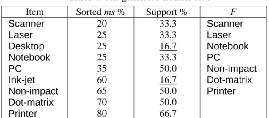
Example 3. Continuing with Example 1, we change ms(Scanner) from 15% to 20%. The resulting F

is shown in Table 4. We observe that ms(Scanner) is the smallest of all items, and Scanner could join with any item whose support is greater than or equal to ms(Scanner) 20% to become a candidate 2-itemset without losing any 2-itemsets. The 2-itemsetsScanner, Desktopand Scanner, Ink-jetcould not become candidates because sup(Desktop) or sup(Ink-jet) is less than ms(Scanner), and the supports of Scanner, Desktopand Scanner, Ink-jetcould not be greater than

sup(Desktop) and sup(Ink-jet), respectively, according to the downward closure property. Therefore,

we keep items whose support is greater than or equal to ms(Scanner) in F, and discard Desktop and Ink-jet.

Table 4. The generated frontier set F.

Item Sorted ms % Support % F

Scanner Laser Desktop Notebook PC Ink-jet Non-impact Dot-matrix Printer 20 25 25 25 35 60 65 70 80 33.3 33.3 16.7 33.3 50.0 16.7 50.0 50.0 66.7 Scanner Laser Notebook PC Non-impact Dot-matrix Printer

Lemma 4. For k3, any k-itemset A = a1, a2,…,akgenerated by procedure apriori-gen(Lk1) can be

pruned if there exists one (k1) subset of A, say ai₁, ai₂,…,ai_k1, such thatai₁, ai₂,…,ai_k1Lk1and

ai1a1or ms(ai1)ms(ai2).

Proof. It is straightforward from the contrapositive statement in Lemma 2. ■

The procedure for generating the set of candidate k-itemsets (k3), called Ck-gen(Lk1), is shown

in Figure 3, which consists of two steps: (1) calling apriori-gen to produce candidate itemsets, and (2) pruning from Ckthose itemsets that satisfy Lemma 4.

Ck= apriori-gen(Lk-1); /* Joins Lk-1with Lk-1*/

for each itemset Aa1, a2,…,akCkdo

for each (k-1)-itemset A’ai₁, ai₂,…,ai_k1of A do

if a1ai₁or ms(ai₁)ms(ai₂) then

if A’Lk-1then delete A from Ck;

Fig. 3. Procedure Ck-gen(Lk1).

3.2 Algorithm MMS_Cumulate

As stated in [11], the main problem arisen from incorporating taxonomy information into association rule mining is how to effectively compute the occurrences of an itemset A in the transaction database

D. This involves checking for each item aA whether a or any of its descendants are contained in a

transaction t. Intuitively, we can simplify the task by first adding the ancestors of all items in a transaction t into t. Then a transaction t contains A if and only if the extended transaction t+contains A. Following the Cumulate algorithm in [11], our MMS_Cumulate is deployed according to this simple concept with the following enhancements:

Enhancement 1. Ancestors pre-computing: instead of traversing the taxonomy T to determine the ancestors for each item, we pre-compute the ancestors of each item. The result is stored as a table called IA.

Enhancement 2. Ancestors filtering: only ancestors that are in one or more candidates of the current

Ckare added into a transaction. That is, any ancestor in IA that is not present in any of the candidates

in Ckis pruned.

Enhancement 3. Itemset pruning: in each Ck, any itemset that contains both an item and its ancestor is

pruned. This is derived from the following observation. Note that the pruning should be performed for each Ck(k2), instead of C2only

1 .

Lemma 5. [11] The support of an itemset A that contains both an item a and its ancestor ais the

same as the support for itemset A{a}.

Proof. The proof is given in [11].

Enhancement 4. Item pruning: an item in a transaction t can be pruned if it is not present in any of the candidates in Ck, as justified by Lemma 4. Note that this should be performed after Enhancement 2.

1 _{The statement of Lemma 2 in [11] is incorrect. For example, consider two itemsets {a, b} and {a, c} in L} 2,

and c is an ancestor of b. Note that b and c are not in the same itemset, but clearly {a, b, c} will be in C3. This

Lemma 6. For k 2, an item a that is not present in any itemset of Lk will not be present in any

itemset of Ck+1.

Proof. This is straightforward from the fact that Ck+1is derived from joining Lkwith Lkfor k2. ■

Indeed, Enhancement 2 is derived from Lemma 6 as well. Because an item may be a terminal or an interior node in the taxonomy graph and the transactions in database D are composed of terminal items only, we have to perform ancestor-filtering first and then item-pruning; otherwise, we will lose the case though some items are not frequent, in contrast to their ancestors. Figure 4 shows an overview of the MMS_Cumulate algorithm. The procedure for generating F is shown in Figure 5. Procedure subset(Ck, t) follows the description in [2] except that items in transaction t are inspected in ascending

ordering of minimum supports, rather than in lexicographic ordering.

Create IMS; /* the table of user-defined minimum support */

Create IA; / * the table of each item and its ancestors from taxonomy T */

SMSsort(IMS); /* ascending sort according to ms(a) stored in IMS */ FF-gen(SMS, D, IA);

L1{a F | sup(a) ms(a)};

for ( k2; Lk1; k) do

if k2 then C2= C2-gen(F);

else CkCk-gen(Lk1);

Delete any candidate in Ckthat consists of an item and its ancestor;

Delete any ancestor in IA that is not present in any of the candidates in Ck;

Delete any item in F that is not present in any of the candidates in Ck;

for each transaction tD do

for each item at do

Add all ancestors of a in IA into t; Remove any duplicates from t;

Delete any item in t that is not present in F;

Ctsubset(Ck, t );

for each candidate ACtdo

Increase the count of A; end for

Lk{A Ck| sup(A)ms(A[1])}; /* A[1] denote the first item in A */

end for ResultkLk;

for each transaction tD do

for each item at do

Add all ancestors of a in IA into t; Remove any duplicates from t;

for each item at do

Increase the count of a; end for

for each item a in SMS in the same order do

if sup(a)ms(a) then

Insert a into F; break;

end if end for

for each item b in SMS that is after a in the same order do

if sup(b)ms(a) then insert b into F;

Fig. 5. Procedure F-gen( SMS, D, IA ).

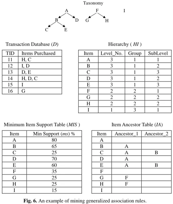
Tables 5 and 6 show the process of applying MMS_Cumulate to the example shown in Figure 6. For simplicity, item “A”standsfor“Printer”,“B”for“Non-impactprinter”,“C”for“Laserprinter”, “D”for“Dot-matrix printer”,“E”for“Ink-jetprinter”,“F”for“PC”,“G”for“Desktop PC”,“H”for “Notebook”,and “I”for“Scanner”in thetaxonomy.

3.3 Algorithm MMS_Stratify

The stratification concept is introduced in [11]. It refers to a level-wise counting strategy from the top level of the taxonomy down to the lowest level, hoping that candidates containing items at higher levels will not have minimum support, thus there is no need to count candidates that include items at lower levels. However, this counting strategy may fail in the case of non-uniform minimum supports.

Example 4. Let {Printer, PC}, {Printer, Desktop}, and {Printer, Notebook} be candidate itemsets

to be counted. The taxonomy and minimum supports are defined as in Example 1. Using the level-wise strategy, we count first {Printer, PC} and assume that it is not frequent, i.e., sup({Printer, PC})0.35. Because the minimum supports of {Printer, Desktop}, 0.25, and {Printer, Notebook}, also 0.25, are less than that of {Printer, PC}, we cannot assure that the occurrences of {Printer, Desktop} and {Printer, Notebook}, though less than {Printer, PC}, are also less than their minimum supports. In this case, we still have to count {Printer, Desktop} and {Printer, Notebook}

even though {Printer, PC} does not have minimum support. Taxonomy I A B D C E F G H

Transaction Database (D) Hierarchy ( HI )

TID Items Purchased Item Level_No. Group SubLevel

11 H, C A 3 1 1 12 I, D B 3 1 2 13 D, E C 3 1 3 14 H, D, C D 3 1 2 15 I E 3 1 3 16 G F 2 2 1 G 2 2 2 H 2 2 2 I 1 3 1

Minimum Item Support Table (MIS ) Item Ancestor Table (IA)

Item Min Support (ms) % Item Ancestor_1 Ancestor_2

A 80 A B 65 B A C 25 C A B D 70 D A E 60 E A B F 35 F G 25 G F H 25 H F I 15 I

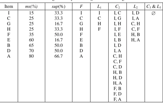
Fig. 6. An example of mining generalized association rules. Table 5. Summary for Itemsets, Counts and Supports of D in Figure 6. 1-itemset Counts sup(%) 2-itemset Counts sup(%) 3-itemset Counts sup(%)

I 2 33.3 I, A 1 16.7 F, B, D 1 16.7 F 3 50.0 I, D 1 16.7 C, F, D 1 16.7 G 1 16.7 F, A 2 33.3 H, B, D 1 16.7 H 2 33.3 F, B 2 33.3 H, C, D 1 16.7 A 4 66.7 F, D 1 16.7 B 3 50.0 C, F 2 33.3 D 3 50.0 C, D 1 16.7 C 2 33.3 H, A 2 33.3 E 1 16.7 H, B 2 33.3 H, C 2 33.3 H, D 1 16.7 B, D 2 33.3 E, D 1 16.7

Table 6. Running summary of MMS_Cumulate on Figure 6.

Item ms(%) sup(%) F L1 C2 L2 C3& L3 I C G H F E B D A 15 25 25 25 35 60 65 70 80 33.3 33.3 16.7 33.3 50.0 16.7 50.0 50.0 66.7 I C G H F E B D A I C H F I, C I, G I, H I, F I, E I, B I, D I, A C, H C, F C, D H, B H, D H, A F, B F, D F, A I, D I, A C, H C, F H, B H, A 

The following observation inspires us to deploy the MMS_Stratify algorithm.

Lemma 7. Consider two k-itemsetsa1, a2,…,akand a1, a2,…,aˆk, where aˆk is an ancestor of ak.

Ifa1, a2,…,aˆkis not frequent, then neither is a1, a2,…,ak.

Proof. Note that ms(a1, a2,…,ak)msa1, a2,…,aˆk)ms(a1). Because sup(ak)sup(aˆk), ifa1, a2,…,aˆkis not frequent we can derive

supa1, a2,…,ak)supa1, a2,…,aˆk)msa1, a2,…,aˆk)ms(a1, a2,…,ak),

which completes the proof. ■

Lemma 7 implies that if a sorted candidate itemset in a higher level of the taxonomy is not frequent, then neither are all of its descendants that differ from the itemset only in the last item. Note that we do not make any relative assumption about the minimum supports of the item ak and its

ancestor aˆk. This means that the claim in Lemma 7 applies to any specifications of ms(ak)ms(aˆk)

(corresponding to uniform case), ms(ak)ms(aˆk), or ms(ak) ms(aˆk) (not ordinary case). As will

become clear later, this makes our counting strategy applicable to any user-specified minimum item support specification.

We first divide Ck, according to the ancestor-descendant relationship claimed in Lemma 7, into

two disjoint subsets, called top candidate set TCkand residual candidate set RCk, defined below.

''denotes don't care. A candidate k-itemset Aa1, a2,…,ak1, akis a top candidate if none of the

candidates in Skis an ancestor of A. That is,

TCk{A | A Ck,(A Ckand A[i]A i[ ], 1i k1, A k[ ] is an ancestor of A[k])},

and

RCk= CkTCk.

Example 5. Assume that the candidate 2-itemset C2 for Example 1 consists of Scanner, PC, Scanner, Desktop, Scanner, Notebook, Notebook, Laser, Notebook, Non-impact, and Notebook, Dot matrix, and the supports of the items in higher levels are larger than those in lower levels. Then TC2{Scanner, PC,Notebook, Non-impact,Notebook, Dot matrix} and RC2 {Scanner, Desktop,Scanner, Notebook,Notebook, Laser}.

Our approach is that, in each pass k, rather than counting all candidates in Ck as in

MMS_Cumulate, we count the supports for candidates in TCk. Then those that do not have minimum

supports are deleted along with their descendants in RCk. If RCkis not empty, we then perform an extra

scan over the transaction database D to count the remaining candidates in RCk. Again, the less frequent

candidates are eliminated. The resulting TCkand RCk, called TLkand RLkrespectively, form the set of

frequent k-itemsets Lk. An overview of the MMS_Stratify algorithm is described in Figure 7. The

enhancements used in MMS_Cumulate apply to this algorithm as well. The procedures for generating

TCkand RCkare given in Figures 8 and 9 respectively, where HI denotes the hierarchy_item relation.

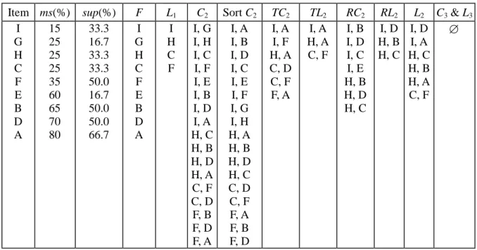
Table 7 shows the progressing result of applying MMS_Stratify to the example in Figure 6.

Example 6. Let us continue with Example 5. If the support of the top level candidate does not pass its

minimum support ms(Scanner), we do not need to count the remaining descendant candidates Scanner, Desktop, Scanner, Notebook. On the contrary, if Scanner, Desktopis a frequent itemset, we should perform another pass over D to count Scanner, Desktopand Scanner, Notebookto determine whether they are frequent or not.

3.4 Analytical comparison of MMS_Cumulate and MMS_Stratify

In this subsection, we will compare the proposed two algorithms in terms of their complexity. Rather than deriving the computation cost to accomplish the whole task, we confine ourselves to the main step: Given the current set of frequent k-itemset Lk, what is the cost to generate the set of frequent

k+1-itemsets Lk+1?

Recall that for Apriori-like algorithms, the set of candidate k+1-itemsets Ck+1 are formed from

Create IMS;

Create HI; /* the table of each item with Hierarchy Level, Sublevel, and Group */ Create IA; SMS = sort(IMS); FF-gen(SMS, D, IA); L1{aF | sup(a) ms(a)}; for (k = 2; Lk1; k++) do if k = 2 then C2= C2-gen(F) else Ck= Ck-gen( Lk1);

Delete any candidate in Ckthat consists of an item and its ancestor;

Delete any ancestor in IA that is not present in any of the candidates in Ck;

Delete any item in F that is not present in any of the candidates in Ck;

TCk= TCk-gen(Ck, HI); /* Using Ck, HI to find top Ck*/

for each transaction tD do

for each item at do

Add all ancestors of a in IA into t; Remove any duplicates from t;

Delete any item in t that is not present in F;

Ct= subset( TCk, t );

for each candidate ACtdo

Increase the count of A; end for

TLk= {ATCk| sup(A)ms(A[1])};

RCk= RCk-gen(Ck, TCk, TLk); /* Using Ck, TLkto find residual Ck*/

if RCkthen

Delete any ancestor in IA that is not present in any of the candidates in RCk;

Delete any item in F that is not present in any of the candidates in RCk;

for each transaction tD do

for each item at do

Add all ancestors of a in IA into t; Remove any duplicates from t;

Delete any item in t that is not present in F;

Ct= subset(RCk, t);

for each candidate ACtdo

Increase the count of A; end for RLk= {ARCk| sup(A)ms(A[1])}; end if Lk= TLkRLk; end for Result = kLk;

for each itemset ACkdo

Sort Ckaccording to HI of A[k] preserving the ordering of A[1]A[2]…A[k-1];

for itemset ACkin the same order do

Sk{ A | A Ckand A[i]A i[ ], 1i k1};

if A is not marked and none of the candidates in Skis an ancestor of A[k] then

Insert A into TCk;

Mark A and all of its descendants in Sk;

end if end for

Fig. 8. Procedure TCk-gen(Ck, HI).

for each itemset ATCkdo

if ATLkthen

Sk= { A | ACkand A[i]A i[ ], 1i k1};

Insert all of its descendants in Skinto RCk;

end if

Fig. 9. Procedure RCk-gen(Ck, TCk, TLk).

Table 7. Running summary of MMS_Stratify on Figure 6.

Item ms(%) sup(%) F L1 C2 Sort C2 TC2 TL2 RC2 RL2 L2 C3& L3 I G H C F E B D A 15 25 25 25 35 60 65 70 80 33.3 16.7 33.3 33.3 50.0 16.7 50.0 50.0 66.7 I G H C F E B D A I H C F I, G I, H I, C I, F I, E I, B I, D I, A H, C H, B H, D H, A C, F C, D F, B F, D F, A I, A I, B I, D I, C I, E I, F I, G I, H H, A H, B H, D H, C C, D C, F F, A F, B F, D I, A I, F H, A C, D C, F F, A I, A H, A C, F I, B I, D I, C I, E H, B H, D H, C I, D H, B H, C I, D I, A H, C H, B H, A C, F 

candidate itemset is counted by scanning the transaction database. In this context, the primary computation involves database scanning and support counting of the candidate itemsets. Let be the

ratio of the cost for scanning a transaction from the database to that for counting the support of an itemset. The cost for the step of concern is |Ck+1||D| for MMS_Cumulate, while for MMS_Stratify

it is |TCk+1||

* 1 

k

RC | + 2|D|, where RC*k1 denotes, after performing the stratification pruning, the set of remaining candidates in RCk+1. Let kmax be the maximal cardinality of frequent itemsets. Then the total cost difference of the two algorithms will be





RC | denotes the number of candidates in RCkpruned by the stratification strategy.

Thus, the result in Eq. 6 means that the superiority of MMS_Stratify over MMS_Cumulate depends on whether the cost reduced by the stratification pruning can compensate for that spent on extra scanning of the database, which will be seen later in the experiments.

4. Experiments

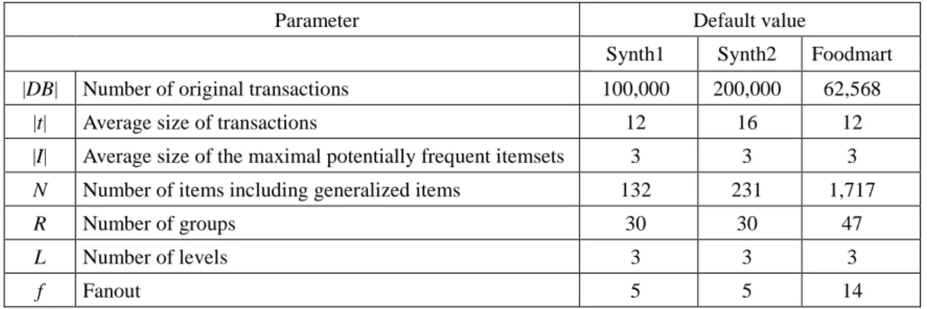
In this section, we evaluate the performance of algorithms, MMS_Cumulate and MMS_Stratify, using two synthetic datasets, named Synth1 and Synth2, generated by the IBM data generator [2, 11], and Microsoft foodmart2000 database (Foodmart for short), a sample supermarket data warehouse provided in MS SQL 2000. The parameter settings are shown in Table 8. The data for Foodmart is drawn from sales_fact_1997, sales_fact_1998 and sales_fact_dec_1998 in foodmart2000. The corresponding item taxonomy consists of three levels: There are 1560 primitive items in the first level (product), 110 generalized items in the second level (product_subcategory), and 47 generalized items in the top level (product_category). All experiments were performed on an Intel Pentium-IV 2.80GHz with 2GB RAM, running on Windows 2000.

Table 8. Parameter settings for synthetic dataset and foodmart2000.

Parameter Default value

Synth1 Synth2 Foodmart |DB| Number of original transactions 100,000 200,000 62,568

|t| Average size of transactions 12 16 12

|I| Average size of the maximal potentially frequent itemsets 3 3 3

N Number of items including generalized items 132 231 1,717

R Number of groups 30 30 47

L Number of levels 3 3 3

f Fanout 5 5 14

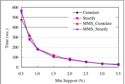
We first compared the execution times of MMS_Cumulate and MMS_Stratify with the Cumulate and Stratify algorithms presented in [11] for different uniform minimum supports, ranging from 0.5%

to 3.5% for Synth1 and Synth2, respectively, and 0.05% to 0.35% for Foodmart. The results are shown in Figures 10 to 12. It can be observed that in uniform support constraint, MMS_Cumulate behaves like its uniform counterpart, Cumulate. However, the situation is somewhat different for MMS_Stratify and Stratify, particular in the real dataset Foodmart, where MMS_Stratify overwhelms Stratify. This is because the definition of ancestor-descendant relationship in MMS_Stratify is more rigorous than that in Stratify. Consequently, during the execution of Stratify, many itemset groups that satisfy the relationship are identified but most of them are frequent. Therefore, as the smaller the support constraint is, the larger the amount of top itemsets identified are frequent, and the longer the amount of time spent on the stratification pruning is wasted. This also explains why Cumulate and MMS_Cumulate perform better than Stratify and MMS_Stratify.

0 100 200 300 400 500 600 0.5 1.0 1.5 2.0 2.5 3.0 3.5 Min Support (%) T im e (s ec .) Cumulate Stratify MMS_Cumulate MMS_Stratify

Fig. 10. Execution times for various minimum supports for Synth1.

0 600 1200 1800 2400 3000 3600 0.5 1.0 1.5 2.0 2.5 3.0 3.5 Min Support (%) T im e (s ec .) Cumulate Stratify MMS_Cumulate MMS_Stratify

0 1000 2000 3000 4000 5000 6000 0.05 0.10 0.15 0.20 0.25 0.30 0.35 Min Support (%) T im e (s ec .) Cumulate Stratify MMS_Cumulate MMS_Stratify

Fig. 12. Execution times for various minimum supports for Foodmart.

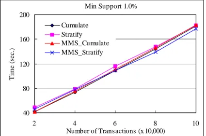
We then compared the scalability of the algorithms under varying transaction sizes at uniform

minsup 1.0% for Synth1 and Synth2, and minsup 0.1% for Foodmart. The results are shown in Figures 13 to 15. As can be seen, all algorithms exhibit good linear scalability. Note that the picture shown in Figure 13 is somewhat different from the others. In particular, MMS_Stratify takes the lead when the transaction size is over 60,000. This is because in this case MMS_Stratify can prune much more candidates through the restricted ancestor-descendant relationship to lessen the work spent on database scanning for support counting.

Min Support 1.0% 40 80 120 160 200 2 4 6 8 10 Number of Transactions (x 10,000) T im e (s ec .) Cumulate Stratify MMS_Cumulate MMS_Stratify

Min Support 1.0% 100 200 300 400 500 600 700 800 4 8 12 16 20 Number of Transactions (x 10,000) T im e (s ec .) Cumulate Stratify MMS_Cumulate MMS_Stratify

Fig. 14. Transactions scale-up for uniform minimum support

with minsup

1.0%

Min Support 0.1% 0 400 800 1200 1600 2000 1 2 3 4 5 6 7 Number of Transactions (x 10,000) T im e (s ec .) Cumulate Stratify MMS_Cumulate MMS_Stratify

Fig. 15. Transactions scale-up for uniform minimum support

with minsup

0.1%

The efficiency of MMS_Cumulate and MMS_Stratify were then compared for multiple minimum supports. Three different specifications discussed in Section 3.2 were examined. They are 1) the support of each item was assigned randomly (random specification); 2) the support of each item was assigned according to Eq. 1 (normal specification); and 3) the support of each item is assigned using Eq. 5 (CLS specification). Note that all of these specifications satisfied the ordinary case that the minimum support of an item a is not larger than that of any of its ancestors aˆ, i.e., ms(a) 

ms(aˆ).This assumption conforms to the fact that the support of an item in the database is less than that of its ancestors. In order to speed up the mining time for normal specification and CLS specification, when ms(a) is less than 0.5%, we set ms(a)0.5% for Synth1 and Synth2, and when ms(a) is less than 0.05%, we set ms(a)0.05% for Foodmart.

For random specification, minimum supports ranging from 0.1% to 6.0% for Synth1 and Synth2 and from 0.011% to 6.0% for Foodmart were specified to items randomly, with items in higher levels

of the taxonomy receiving larger values. The results are shown in Figures 16 to 18. Algorithm MMS_Cumulate performs better than MMS_Stratify, with the gap increasing as the number of transactions increases. The results also display the scalability of the algorithms. Both MMS_Cumulate and MMS_Stratify exhibit linear scale-up with the number of transactions.

Figures 19 to 21 show the results for the normal specification. Overall, MMS_Cumulate performs better than MMS_Stratify, but the gap decreases as is getting larger. However, in Figure 19, MMS_Stratify performs slightly worse than MMS_Cumulate for  0.3 but overwhelms MMS_Cumulate when is larger than 0.3. This is because we have set ms(a)0.5% when ms(a) is less than 0.5%, causing many top itemsets to be infrequent. Therefore, MMS_Stratify can prune much more low-level candidates.

For CLS specification, similar results can be observed, as shown in Figures 22, 23 and 24.

Finally, we examined the capability of the proposed methods in finding informative rules with small and non-uniform supports. To this end, we chose some items of high values but with relative small supports in Foodmart, as shown in Table 9, and tried to find informative rules composed of these items. Notethattheitem “Cereal”isageneralized item whiletheothersareprimitiveitems. We have used the following setting. The minimum supports were set as ms(Pleasant Canned Yams)  0.005%, ms(Gorilla Mild Cheddar Cheese)  0.25%, ms(Carrington Ice Cream)  0.25%,

ms(CDR Apple Preserves) = 0.002%, ms(Giant Small Brown Eggs) = 0.25%, ms(Cereal) = 3%,

and was randomly set within 0.2% to 6% for other items. The minimum confidence was set to be 60%.

20 40 60 80 100 120 140 160 2 4 6 8 10 Number of Transactions (x 10,000) T im e (s ec .) MMS_Cumulate MMS_Stratify

0 200 400 600 800 1000 4 8 12 16 20 Number of Transactions (x 10,000) T im e (s ec .) MMS_Cumulate MMS_Stratify

Fig. 17. Execution time for random support specification for Synth2.

0 40 80 120 160 200 240 1 2 3 4 5 6 7 Number of Transactions (x 10,000) T im e (s ec .) MMS_Cumulate MMS_Stratify

Fig. 18. Execution time for random support specification for Foodmart.

0 50 100 150 200 250 300 350 0.1 0.2 0.3 0.4 0.5  T im e (s ec .) MMS_Cumulate MMS_Stratify

0 200 400 600 800 1000 1200 0.1 0.2 0.3 0.4 0.5  T im e (s ec .) MMS_Cumulate MMS_Stratify

Fig. 20. Execution times for normal support specification for Synth2.

0 400 800 1200 1600 2000 0.1 0.2 0.3 0.4 0.5  T im e (s ec .) MMS_Cumulate MMS_Stratify

Fig. 21. Execution times for normal support specification for Foodmart.

0 50 100 150 200 250 300 350 0.1 0.2 0.3 0.4 0.5 0.6 0.7 0.8 0.9 Min Confidence T im e (s ec .) MMS_Cumulate MMS_Stratify

0 200 400 600 800 1000 1200 0.1 0.2 0.3 0.4 0.5 0.6 0.7 0.8 0.9 Min Confidence T im e (s ec .) MMS_Cumulate MMS_Stratify

Fig. 23. Execution time for CLS support specification for Synth2.

0 400 800 1200 1600 0.1 0.2 0.3 0.4 0.5 0.6 0.7 0.8 0.9 Min Confidence T im e (s ec .) MMS_Cumulate MMS_Stratify

Fig. 24. Execution time for CLS support specification for Foodmart.

Table 9. Selected high-value items with small supports from Foodmart.

Itemset Support

Pleasant Canned Yams 0.237%

Carrington Ice Cream 0.272%

Gorilla Mild Cheddar Cheese 0.328%

CDR Apple Preserves 0.128%

Giant Small Brown Eggs 0.257%

Cereal 5.391%

Some interesting rules were discovered, but for simplicity, we only show four of them. The first two discovered rules were generated from the frequent itemset {Pleasant Canned Yams, Carrington Ice Cream, Gorilla Mild Cheddar Cheese} as shown below:

Pleasant Canned Yams, Carrington Ice Cream  Gorilla Mild Cheddar Cheese (sup  0.008%, conf83.3%, lift = 306.7)

and

Pleasant Canned Yams, Gorilla Mild Cheddar Cheese  Carrington Ice Cream (sup  0.008%, conf100%, lift = 305.2).

Another two were generated from the frequent itemset {CDR Apple Preserves, Giant Small Brown Eggs, Cereal}:

CDR Apple Preserves, Giant Small Brown Eggs Cereal (sup = 0.003%, conf = 66.7%, lift = 12.4)

and

CDR Apple Preserves, Cereal Giant Small Brown Eggs (sup = 0.003%, conf = 50%, lift = 194.3).

All of these rules exhibit high confidence and positive implication. In reality, these rules reveal that the promotion of some item combinations, e.g., Pleasant Canned Yams and Gorilla Mild Cheddar Cheese, is very likely to raise the sales of some particular items, e.g., Carrington Ice Cream. Simple though this example is, it has illustrated the ability of our methods in finding very rare but informative rules.

5. Related Work

The problem of mining association rules in the presence of taxonomy information was addressed first in [5] and [11]. In [11], the problem isnamed “mining generalized association rules,”which aims to find associations between items at any level of the taxonomy under the minsup and minconf constraints. Their work, however, did not recognize the varied support requirements inherent in items at different hierarchy levels.

In [5], the problem was stated somewhat different from that in [11]. They generalized the uniform minimum support constraint into a form of level-wise assignment, i.e., items at the same level receive the same minimum support. The objective was mining associations level-by-level in a fixed hierarchy. That is, only associations between items at the same level were examined progressively from the top level to the bottom.

Another form of association rules involving mining with multiple minimum supports was proposed in [7]. Their method allows users to specify different minimum support for different items and can find rules involving both frequent and rare items. However, their model considers no taxonomy at all and hence fails to find associations between items at different hierarchy levels.

To our knowledge, [5] is the only work considering both aspects of item taxonomy and multiple supports. However, their intention was quite different from ours. First, although several variants were proposed, all of them follow a level-wise, progressively deepening strategy that performs a top-down traversing of the taxonomy to generate all frequent itemsets. An Apriori-like algorithm is applied at each level, which leads to p database scans, where plkland klis the maximum k-itemset at level l.

This is quite a large overhead compared with our algorithm, which requires only maxlkltimes. Second,

the minimum supports are specified uniform at each taxonomy level, that is, items at the same taxonomy level receive the same minimum support. This restrains the flexibility and power of association rules. Furthermore, together with the progressively deepening strategy, their approaches would fail to discover all frequent itemsets, especially those involving level-crossing associations. Let us illustrate this with an example, and for self-explanatory demonstration, a generic description of their approaches is given in Figure 25.

Ď: a taxonomy-information-encoded transaction database;

minsup[l]: the minimum support threshold for each concept level l;

for (l = 1; L[l, 1]and l < max_level; l++) do

L[l, 1] = the frequent 1-itemsets at level l;

for (k = 2; L[l, k1] ; k++) do

Ckapriori-gen(L[l, k 1]);

for each transaction tĎdo

Ct= subset(Ck, t);

for each candidate ACtdo increase the count of A;

endfor

L[l, k] = {ACk| sup(A)minsup[l]};

endfor

LL[l] = kL[l, k]; /* LL[l]: the set of frequent itemsets at level l */

end for

ResultlLL[l];

Fig. 25. A generic description of multi-level association mining algorithms presented in [5].

Example 7. Consider the example used in [5], as shown in Figure 26, where the minimum support is

set to be 4 at level 1, and 3 at levels 2 and 3. Each item is encoded as a sequence of digits, representing its positions in the taxonomy. For example, the item ‘White Old Mills Bread’is encoded as ‘211’in which the first digit, ‘2’, represents ‘bread’at level-1, the second ‘1’for ‘White’at level 2, and the third ‘2’for ‘Old Mills’at level 3. To discover all frequent itemsets, the proposed algorithms first apply the Apriori algorithm to T, generating all level-1 frequent itemsets. The result is

L[1, 1]{{1* *}, {2* *}}, and

L[1, 2]{{1* *, 2* *}}.

According to the level-wise deepening paradigm, only descendants of the frequent itemsets at level-1 are inspected to generate frequent itemsets at level-2. The resulting level-2, frequent 1-itemset is

L[2, 1]{{11*}, {12*}, {21*}, {22*}}.

Note that {32*} and {41*} are missed in L[2, 1] though they are frequent. For the same reason, {323} is missed in L[3, 1] and so are level-crossing frequent itemsets {111, 12 *}, {12 *, 221}, {11 *, 12 *, 221}. Food

...

..

..

..

..

tid Items Purchased

11 {111, 121, 211, 221} 12 {111, 211, 222, 323} 13 {112, 122, 221, 411} 14 {111, 121} 15 {111, 122, 211, 221, 413} 16 {211, 323, 524} 17 {323, 411, 524, 713}

Fig. 26. The example of taxonomy and encoded transaction table in [5].

6. Conclusions

We have investigated in this paper the problem of mining generalized association rules in the presence of taxonomy and multiple minimum support specification. The classic Apriori itemset generation works in the presence of taxonomy but fails in the case of non-uniform minimum supports. We presented two algorithms, MMS_Cumulate and MMS_Stratify, for discovering these generalized frequent itemsets. Empirical evaluation showed that these two algorithms are very effective and have good linear scale-up characteristic. Between the two algorithms, MMS_Stratify performed slightly

better than MMS_Cumulate, with the gap increasing with the problem size, such as the number of transactions and/or candidate itemsets. As for the specification for non-uniform, multiple item supports, we also presented a confidence-lift specification, which is beneficial for discovering less-supported but perceptive rules without suffering from combinatorial explosion.

References

[1] R. Agrawal, T. Imielinski, and A. Swami, Mining association rules between sets of items in large databases, in: Proc. 1993 ACM-SIGMOD Int. Conf. on Management of Data, (Washington, D.C., 1993) 207-216.

[2] R. Agrawal and R. Srikant, Fast algorithms for mining association rules, in: Proc. 20th Int. Conf. on Very Large Data Bases, (Santiago, Chile, 1994) 487-499.

[3] S. Brin, R. Motwani, and C. Silverstein, Beyond market baskets: generalizing association rules to correlations, in: Proc. 1997 ACM-SIGMOD Int. Conf. on Management of Data, (1997) 207-216. [4] S. Brin, R. Motwani, J. D. Ullman, and S. Tsur, “Dynamicitemsetcounting and implication rules

for market-basket data,”in:Proc. 1997 ACM-SIGMOD Int. Conf. on Management of Data, (1997) 207-216.

[5] J. Han and Y. Fu, Discovery of multiple-level association rules from large databases, in: Proc. 21st Int. Conf. on Very Large Data Bases, (Zurich, Switzerland, 1995) 420-431.

[6] W. Y. Lin, M. C. Tseng, and J.H.Su,“A confidence-lift support specification for interesting associationsmining,”in: Proc. 6th Pacific Area Conference on Knowledge Discovery and Data Mining (PAKDD-2002), Taipei, Taiwan, R.O.C., May 2002.

[7] B.Liu,W.Hsu,and Y.Ma,“Mining association ruleswith multipleminimum supports,”in:Proc. 1999 Int. Conf. on Knowledge Discovery and Data Mining, (San Deige, CA, 1999) 337-341. [8] B. Lin, W. Hsu, and Y. Ma, Pruning and summarizing the discovered association, in: Proc. 1999

ACM-SIGKDD Int. Conf. on Knowledge Discovery and Data Mining. (San Diego, CA, 1999) 125-134.

[9] J.S.Park,M.S.Chen,and P.S.Yu,“An effectivehash-based algorithm for mining association rules,”in:Proc. 1995 ACM-SIGMOD Int. Conf. on Management of Data, (San Jose, CA 1995) 175-186.

[10] A.Savasere,E.Omiecinski,and S.Navathe,“An efficientalgorithm for mining association rules in largedatabases,”in: Proc. 21st Int. Conf. on Very Large Data Bases, (Zurich, Switzerland, 1995) 432-444.

[11] R.Srikantand R.Agrawal,“Mining generalized association rules,”Future Generation Computer Systems, Volume 13, Issues 2-3, November 1997, 161-180.