以視覺為基礎之戶外全天停車場空位偵測系統

國 立 交 通 大 學

電子工程學系 電子研究所碩士班

碩

士

論

文

以視覺為基礎之戶外全天停車場空位偵測系統

A Vision-based Vacant Parking Space Detection

Framework for All-Day Outdoor Parking Lot

Management

研 究 生：戴玉書

指導教授：王聖智 博士

以視覺為基礎之戶外全天停車場空位偵測系統

A Vision-based Vacant Parking Space Detection Framework

for All-Day Outdoor Parking Lot Management System

研 究 生：戴玉書 Student：Yu-Shu Dai

指導教授：王聖智博士 Advisor：Dr. Sheng-Jyh Wang

國 立 交 通 大 學

電子工程學系 電子研究所碩士班

碩 士 論 文

A Thesis

Submitted to Department of Electronics Engineering & Institute of Electronics College of Electrical and Computer Engineering

National Chiao Tung University in partial Fulfillment of the Requirements

for the Degree of Master of Science in

Electronics Engineering August 2011

Hsinchu, Taiwan, Republic of China

以視覺為基礎之戶外全天停車場空位偵測系統

研究生：戴玉書 指導教授：王聖智 博士

國立交通大學

電子工程學系 電子研究所碩士班

摘要

在本論文中，我們提出一套可以全天二十四小時運作的戶外停車

場空位偵測系統。特別針對夜晚的情況，我們設計出一種動態調整曝

光值的取像方式，能同時將多張不同曝光值的影像，經融合處理後得

到一張資訊較完整的融合影像。接著，藉由把整個停車場看成一種面

與面的結構組合、結合 BHF 模型和 3D 場景中車輛的幾何資訊、利

用以 HOG 為基礎的擷取方式，我們擷取出融合影像內各個面相所對

應的特徵向量。最後，把每個面所擷取出的特徵向量以機率模型的方

式，分別比對出每種不同組合的停車假設，而與特徵內容最符合的假

設狀態即為我們的偵測結果。透過本系統，我們可以穩定的分析出停

車場的停車狀況，並提供停車場內空位的位置資訊。

A Vision-based Vacant Parking Space Detection

Framework for All-Day Outdoor Parking Lot

Management

Student: Yu-Shu Dai Advisor: Dr. Sheng-Jyh Wang

Department of Electronics Engineering, Institute of Electronics

National Chiao Tung University

Abstract

In this thesis, we propose a vacant parking space detection system

that works 24 hours a day. Especially, to capture images at night, we

design a capture mode that takes images under different exposure settings

and fuses these multi-exposure images into a clearer image. Besides, we

combine a proposed Bayesian hierarchical framework (BHF) with the

3D-scene information by treating the whole parking lot as a structure

consisting of plentiful surfaces. With the proposed framework, we extract

feature vectors from each surface based on a modified version of the

Histogram of Oriented Gradients (HOG) approach. By incorporating

these feature vectors into specially designed probabilistic models, we can

estimate the current parking status by finding the optimal statistical

hypothesis among all possible status hypotheses. Experiments over real

parking lot scenes have shown that our system can reliably detect vacant

parking spaces day and night on an outdoor parking lot.

誌謝

在此，我要先感謝我的父母，有你們的支持與鼓勵，我才能有今日的

結果。接著要感謝我的指導教授 王聖智 老師，在與您的學習中，我

不但學到了許多課業上的知識和做研究的態度，更重要的是，我學到

了如何獨立地做好每件事情，也了解到從不同角度去看問題本質的重

要性，藉此培養了我獨立思考的能力。感謝實驗室裡的每個成員，感

謝敬群、禎宇、慈澄學長們平時對我的許多幫助，給了我很多在研究

和人生上的思考方向，也感謝韋弘、開暘、鄭綱、郁霖，平時的幫忙

和鼓勵，整個求學生涯中，因為有你們，增添了不少色彩，特別感謝

鄭綱在實驗上的幫忙，以致於讓我可以順利完成論文，還要感謝實驗

室的學弟妹們，秉修、彥廷、柏翔、心憫，有你們在的實驗室裡充滿

歡笑。最後，感謝每一個曾幫助過我的人，謝謝。

Content

Chapter 1. Introduction ... 1

Chapter 2. Background ... 3

2.1. Outdoor Vacant Parking Space Detection Algorithms ... 3

2.1.1. Car-driven Methods ... 4

2.1.2. Space-driven Methods ... 9

2.2. Vision-based Techniques for Night Period ... 14

Chapter 3. Proposed Method ... 18

3.1. Basic Concepts ... 18

3.1.1. Improvement of Night-Period Images ... 19

3.1.2. Combination of Car-driven and Space-driven Methods ... 20

3.2. Detection Algorithm of the Proposed System ... 24

3.2.1. Image Capture System ... 25

3.2.2. Exposure Fusion... 26

3.2.3. Feature Extraction ... 28

3.2.4. Distributions of Surface Patterns ... 32

3.2.5. Inference of Parking Statuses ... 33

3.3. Training Process ... 36

3.4. Implementation Details ... 40

Chapter 4. Experimental Results ... 42

Chapter 5. Conclusions ... 51

List of Figures

Figure 2-1 Two different viewpoints of human face in [1] ... 4

Figure 2-2 Classification algorithm by using local operators in [1] ... 4

Figure 2-3 (a) Eight different viewpoints of cars (b) Detection results in [1] ... 5

Figure 2-4 Two different features of human face in [2] ... 6

Figure 2-5 Schematic depiction of the detection process in [2] ... 6

Figure 2-6 (a) An input image (b) The HOG feature according to the input image in [3] ... 7

Figure 2-7 Detection procedure of [14] ... 7

Figure 2-8 Detection procedure of [4] ... 8

Figure 2-9 Experimental results of [4] ... 8

Figure 2-10 (a) Input image (b) Reconstruction of an empty parking lot (c) Different image (d) The input image with highlighted objects ... 9

Figure 2-11 Flowchart of [6] ... 10

Figure 2-12 (a) Segmentation results of two image patches (b) The analyses of an image patch ... 10

Figure 2-13 (a) Input image patch (b) The weight map of input image patch (c) The segmentation result without the weighting map (d) The segmentation result with the weighting map in [8] ... 11

Figure 2-14 (a) Original image (b) The projected image in [9] ... 11

Figure 2-15 Eight classes of parking space patterns in [11] ... 12

Figure 2-16 The BHF model in [15] ... 13

Figure 2-17 Details between the scene layer, the observation layer, and the hidden-label layer in [15] ... 13

Figure 2-18 (a) An image of the parking lot at daytime (b) An image of the parking lot at night ... 14

Figure 2-19 (a) Original image (b) SSR processing result (c) HSISSR processing result in [16] ... 15

Figure 2-20 Flowchart in [17] ... 16

Figure 2-21 (a)(b) Images at night (b)(e) Results from the two-layer detector (red: candidate position, black: detected cars) (c)(f) Results from the AdaBoost cascade detector (blue: missing cars, black: detected cars) ... 16

Figure 2-22 A three level structure in [19] ... 17

Figure 2-23 (a) Input frames (b) Result of GMM (c) Result of LBP (c) Result of [19] ... 17

Figure 3-1 An image of the parking lot at night ... 19

Figure 3-3 The parking lot with serious occlusions ... 20

Figure 3-4 (a) Car-level data (b) Patch-level data (c) Ground surfaces. (d) Car surfaces ... 21

Figure 3-5 Six surfaces of parking spce ... 21

Figure 3-6 Possible patterns at each surface of the parking space ... 22

Figure 3-7 Structural diagram of the surface-based detection framework... 22

Figure 3-8 Inference flow of the proposed algorithm ... 23

Figure 3-9 Flowchart of the proposed algorithm ... 24

Figure 3-10 The camera settings of AXIS M1114, where the setting of exposure value is marked by the red rectangular ... 25

Figure 3-11 Details of our image capture system ... 26

Figure 3-12 (a) The captured image with EV=10 (b) The captured image with EV=50 (c) The captured image with EV=90 ... 26

Figure 3-13 The procedure of pyramid-based exposure fusion ... 27

Figure 3-14 (a) An Image sequence and its weighting maps (b) The fusion result ... 28

Figure 3-15 The fusion result of images in Figure 3-12 ... 28

Figure 3-16 Comparison of gradient magnitudes between the original image and the fused image (a) The gradient magnitude of the original image (b) The gradient magnitude of the fused image ... 28

Figure 3-17 The six surfaces and the corresponding image regions of a parking space ... 29

Figure 3-18 Image regions of the side surface at four different parking spaces ... 29

Figure 3-19 Normalization of image regions ... 30

Figure 3-20 Normalized image patches of the side surfaces at four different parking spaces ... 30

Figure 3-21 An image patch consisting of many cells ... 31

Figure 3-22 Extraction of HOG features ... 31

Figure 3-23 (a) Original image. (b) HOG features ... 31

Figure 3-24 (a) (a) The definition of super-cell (b) An example of merging a region of 4x8 cells to 2x2 super-cells ... 32

Figure 3-25 Possible patterns of each surface at a parking space ... 33

Figure 3-26 Three blocks in our parking lot ... 33

Figure 3-27 The BHF model of a parking block... 34

Figure 3-28 The inference process of our proposed method ... 35

Figure 3-29 Labels according to different patterns of surfaces ... 37

Figure 3-30 An illustration of the difference between PCA and LDA ... 37

Figure 3-31 Distributions of the "T_1" and "T_2" patterns of the top surface ... 39

Figure 3-33 Row-wise detection procedure ... 40 Figure 3-34 (a) A car parked too inside of the parking space (b) A car parked too outside of the parking space ... 41 Figure 3-35 Three sampling positions of feature extraction for the front surface ... 41 Figure 4-1 (a) An image of the parking lot (b) The corresponding detection regions.42 Figure 4-2 Image samples captured in (a) normal day, (b)sunny day, (c) cloudy day, and

(d)rainy day ... 43 Figure 4-3 (a)(c)(e): Images with shadow effect. (b)(d)(f): The corresponding detection result ... 44 Figure 4-4 (a)(c)(e): Images with different lighting condition. (b)(d)(f): The corresponding detection results ... 45 Figure 4-5 Three images captured under different weather conditions in Huang’s dataset [15] (a) Normal day (b) Sunny day (c) Cloudy day ... 46 Figure 4-6 (a)(c)(e): Different fusion images at light (b)(d)(f): The corresponding detection results ... 47 Figure 4-7 (a)(b) Night period detection with moving cars in the scene Row 1: image samples with EV=10, EV=50, and EV=90 Row 2: Fused images and the corresponding detection result ... 48

List of Tables

Table 4-1 Day period performance of the proposed method ... 43

Table 4-2 Comparisons of day period performance ... 46

Table 4-3 Night period performance of the proposed method ... 48

Table 4-4 Performance between two different approaches in day period ... 49

Table 4-5 Performance between two different approaches in night period ... 50

Table 4-6 Day-period performance over different training sets ... 50

Chapter 1.

I

NTRODUCTION

Due to the rapid development of automotive industry, plentiful vehicles appear in the world and the car parking problem has become a big issue. Up to now, many research works have being focusing on developing intelligent parking management systems that can indicate to the users where to park their cars in the parking lot. With such an intelligent parking management system, a driver can take less time in finding a vacant parking space within a large-scale sparking lot.

Roughly speaking, there are two major approaches for outdoor vacant parking space detection: sensor-based approach and vision-based approach. The sensor-based approach is to place a sensor device, such as infrared sensor, microwave radar or inductive loop, at each parking space of the parking lot. When a car is parked at the parking space, the sensor at that parking space will sense a change. By sending the information to the control room, the parking lot management system can tell the users which parking spaces have already been parked. Although the accuracy of a sensor-based system is usually high, this type of system suffers from some problems in an outdoor parking lot. For example, these sensor devices installed in an outdoor environment may deteriorate or even get damaged by some external factors. Moreover, it is expensive to install sensor devices at every parking space in a large-scale sparking lot. Due to these aforementioned drawbacks, the vision-based approach could be a more attractive and practical choice for a large-scale out-door parking scene.

Different from the sensor-based approach, the vision-based approach uses cameras to capture images of the parking lot. By applying an appropriate detection algorithm over the captured images, the system can monitor the parking situation of the parking lot without installing any other kinds of sensors. Moreover, with only a few cameras, the vision-based approach can monitor all the parking spaces inside the parking lot and is more economical than the sensor-based approach. On the contrary, the accuracy of the vision-based approach depends heavily on the adopted detection algorithm. At present, even though many algorithms have been proposed for vision-based vacant parking space detection, none of them can robustly and accurately detect vacant parking space day and night.

In this thesis, we develop a vision-based vacant parking space detection system, which can work 24 hours a day. In the proposed system, we first design a capture mode which takes images under different exposure settings and then fuses these multi-exposure images into a clearer image. Next, we combine a proposed Bayesian hierarchical framework (BHF) with the 3D-scene information by treating the whole parking lot as a structure consisting of plentiful surfaces. With the proposed framework, we build a vision-based detection system that can robustly detect vacant parking space day and night.

In this thesis, we will first discuss in Chapter 2 some related works for vision-based vacant parking space detection and some vision-based techniques that deal with the dark environments at night. In Chapter 3 we will present the two main ideas of our proposed system. Some experimental results are shown in Chapter 4. Finally, we give our conclusion in Chapter 5.

Chapter 2.

B

ACKGROUND

As we discussed before, there are four main challenges in vision-based parking space detection. They are occlusion effect, shadow effect, perspective distortion, and fluctuation of light condition. In this Chapter, we divide the introduction of existing algorithms into two parts. In the first section, we will introduce some algorithms that are mainly designed to perform vision-based parking space detection during the day. We will also explain how these algorithms deal with occlusion effect, shadow effect, perspective distortion, and fluctuation of light condition. Since we aim to develop a system that can work 24 hours a day, we will also introduce in the second section of this chapter a few existing techniques that are especially designed to deal with the dark environments at night.

2.1. O

UTDOOR

V

ACANT

P

ARKING

S

PACE

D

ETECTION

A

LGORITHMS

There are a lot of ways to detect vacant parking space via vision-based algorithms. In general, these algorithms can be roughly divided into two categories: car-driven methods and space-driven methods. In a car-driven method, the algorithm focuses on finding cars at the parking area. Once a car is found at a parking spot, that parking spot is occupied. Hence, by detecting cars at each parking spot, we can get the present situation of the parking lot. On the contrary, a space-driven method focuses on analyzing the textures or colors of each parking spot. In this approach, the status of the parking spots is detected directly.

2.1.1. C

AR

-

DRIVEN

M

ETHODS

In a car-driven method, we check each of the parking spaces to find whether there is a car at that parking spot. In [1], the author proposed an object detection method by training suitable classifiers based on the data collected from different viewing angles of the target object. Figure 2-1 shows an example of human faces from the front-view angle and the side-view angle.

Figure 2-1 Two different viewpoints of human face in [1]

In [1], for the training of each classifier, the authors use several operators to capture the local information so that the algorithm can be more flexible in dealing with deformations. An example of this approach is shown in Figure 2-2.

Moreover, in [1], the authors propose the use of different classifiers to improve the robustness of object detection. In Figure 2-3, we show the application of the algorithm in [1] to the problem of vehicle detection. In (a), we show the 8 different viewpoints of cars. In (b), we the detection result of the algorithm in [1].

(a)

(b)

Figure 2-3 (a) Eight different viewpoints of cars (b) Detection results in [1]

On the other hand, the authors in [2] propose a robust face detection method by combining various kinds of features and by using the AdaBoosting technique. The same structure can be used for vehicle detection. In Figure 2-4, we show two features adopted in the detection of human face. In Figure 2-5, we show the schematic depiction of the detection process.

Figure 2-4 Two different features of human face in [2]

Figure 2-5 Schematic depiction of the detection process in [2]

For complicated backgrounds, directly using features extracted from images may not work very well. In [3], the authors use a statistical approach to deal with this situation. By computing the histogram of oriented gradients (HOG) of image patches, the boundary characteristics of objects can be better preserved. Figure 2-6 shows an example of an image patch and its HOG feature. By considering each local part of the target object, [14] adopts modified HOG feature and proposes a part-based HOG model to deal with the detection of deformable objects. Figure 2-7 shows the detection procedure of the part-based detection framework. This HOG-based method works well in general cases and can be well applied to the detection of vehicles.

(a) (b)

Figure 2-6 (a) An input image (b) The HOG feature according to the input image in [3]

Based on vehicle detection, [4] uses a more general method to find cars in an image. The authors use color features to find the rough position of candidates within the whole image first. After that, they use edge features, corner features, and wavelet-based texture features to double check whether there is a car at each of these candidate positions. Some details and experimental results are shown in Figure 2-8 and Figure 2-9, separately.

Figure 2-8 Detection procedure of [4]

Figure 2-9 Experimental results of [4]

Even thought the car-driven approach performs very well in a lot of cases, it is still not suitable for outdoor vacant parking space detection. For example, an object may only be partly observed due to the occlusion effect. Cars far away from the camera may appear too small or too distorted to be detected. Nevertheless, the object-driven approach may still perform well over the cases with shadow effect or fluctuation of lighting condition. This is because this approach detects objects by checking the characteristics of objects.

2.1.2. S

PACE

-

DRIVEN

M

ETHODS

Because the surveillance cameras installed in the parking area are typically static, an easy way to extract the information of the parking space is to perform background subtraction. By modeling the background of the camera’s view, we can extract the foreground of each captured image. The foreground of an image is considered as the vehicles parked in the parking space. Hence, by checking the foreground information, it would be easy to determine whether a parking spot is vacant or parked. However, due to the environmental variations, building a background image is not simple. In [5], the author proposes an approach to model the background by using the Principal Component Analysis (PCA) method. By using the PCA technique, the authors can efficiently extract the foreground objects in the image. Figure 2-10 shows a result of that work. Unfortunately, there are still some problems in background subtraction, such as the occlusion effect and the shadows cast by neighboring cars.

(a) (b)

(c) (d)

Figure 2-10 (a) Input image (b) Reconstruction of an empty parking lot

(c) Difference image (d) The input image with highlighted objects

In order to overcome the aforementioned problems, a few researchers try to add in some information about the 3D scene. For example, by using the models of cars and grounds, the method proposed in [6] can deal with the occlusion problem and the

shadow effect. However, when the illumination variation is complicated, this approach may fail. In Figure 2-11, we show the flowchart of this method.

Figure 2-11 Flowchart of [6]

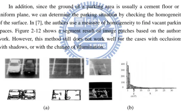
In addition, since the ground of a parking area is usually a cement floor or a uniform plane, we can determine the parking situation by checking the homogeneity of the surface. In [7], the authors use a measure of homogeneity to find vacant parking spaces. Figure 2-12 shows a segment result of image patches based on the authors’ work. However, this method still does not work well for the cases with occlusions, with shadows, or with the change of illumination.

(a) (b)

Figure 2-12 (a) Segmentation results of two image patches (b) The analyses of an image patch

In [8], the authors propose a method similar to [7] to roughly solve the occlusion problem. By adding an occlusion prior, they can know which area will be occupied and they can pay more attention to the other parts. Figure 2-13 shows some details of this approach. However, this method may still suffer from the shadow effect, perspective distortion, and the change of illumination.

(a) (b) (c) (d) Figure 2-13 (a) Input image patch (b) The weight map of input image patch (c) Thesegmentation

result without the weighting map (d) The segmentation result with the weighting map in [8]

With perspective distortion, it becomes more difficult to analyze the characteristics of the parking space. A parking spot far away from the camera will be heavily distorted and this fact makes the detection result less reliable. To handle this problem, the authors in [9] use a calibration technique to convert the original viewpoint to the bird-eye viewpoint. With this conversion, they can roughly solve the perspective distortion problem. Figure 2-14 shows a result of this calibration method.

(a) (b)

Figure 2-14 (a) Original image (b) The projected image in [9]

Another way to do the vacant parking space detection is by using a SVM classifier to classify each parking spot, like the method proposed in [10]. But the change of illumination and the occlusion effect among cars still cause problems. In [11], the authors propose an approach similar to that in [10]. To overcome the perspective distortion of cameras, the authors use a calibration technique to transform the image to the top-view image at first. Second, to deal with the occlusion problem, the author divides the parking space into eight classes by considering a set of three neighboring parking spots sat the same time. After that, by using a SVM classifier, the parking status is estimated. Figure 2-15 shows the eight-class patterns of this work. This method can roughly deal with the occlusion problem and the perspective distortion problem, but may fail in the cases with the change of illumination or with the interference of shadows.

Figure 2-15 Eight classes of parking space patterns in [11]

In [15], the authors combine the detection algorithm with 3D scene information by using a Bayesian hierarchical framework (BHF), which is illustrated in Figure 2-16. By using the angle of the sunlight direction and the car model, the authors apply some constraints over the hidden labels that denote the object status and the illumination status. The object status could be either “car” or “ground”, while the illumination status could be either “shadowed” or “not shadowed”. Finally, by combining with the messages passed from the observation layer, they can determine whether a parking spot is vacant or parked.Figure 2-17 shows some details about the scene layer, the observation layer, and the hidden-label layer of the BHF framework in [15]. Although this method can effectively deal with the aforementioned four major problems in vacant parking space detection, it has difficulty in handling the situations when the shadows come from a moving object or a waiving tree or when the fluctuation of lighting condition are dramatic.

Figure 2-16 The BHF model in [15]

2.2. V

ISION

-

BASED

T

ECHNIQUES FOR

N

IGHT

P

ERIOD

In the previous section, we have introduced several kinds of methods for vision-based parking space detection. However, none of them can perform the detection task day and night. In our system, we aim to develop a system that can also robustly detect vacant parking spaces during the night period. Hence, in this section, we will mention a few vision-based algorithms that are especially designed for dark environments.

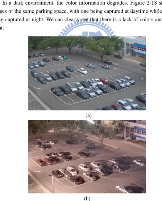
In a dark environment, the color information degrades. Figure 2-18 shows two images of the same parking space, with one being captured at daytime while the other being captured at night. We can clearly see that there is a lack of colors and edges at night.

(a)

(b)

In [16], the authors propose a method to enhance images captured at night. Different from traditional enhancement approaches, the authors transform the RGB color space into the HSI space and only apply the SSR (Single-Scale Retinex) or MSR (Multi-Scale Retinex) algorithm to the S (Saturation) and I (Intensity) components. This is because the authors believe that preserving the H (Hue) component can maintain most color information of the original image. Figure 2-19 shows a performance comparison between the original SSR method and the authors’ work.

(a) (b) (c)

Figure 2-19 (a) Original image (b) SSR processing result (c) HSISSR processing result in [16] With the same concept, the authors in [17] use another method to enhance the image. At first, given a set of day-time images and night-time images, the author decomposes each image into a reflectance term and an illumination term based on the Retinex theory. For the decomposed data, the authors train the ratio of illumination between day-time images and night-time images. After that, the author can decompose each given image into a reflectance term and an illumination term and then modify the illumination term based on the trained ratio. By combining the reflectance term and the modified illumination term, they can get an enhanced image. The procedure of this work is illustrated in Figure 2-20.

On the other hand, based on detected vehicles, [18] uses a two-layer detector to measure the traffic flow at night. At first, the authors identify the candidate positions of vehicles by finding headlights. After that, they use the AdaBoost cascade classifier at each candidate position to determine whether there is a vehicle at that location. Compared to the original AdaBoost cascade classifier, this method is more efficient and can reduce the false positive rate effectively. Figure 2-21 shows the comparison of detection results between this two-layer detector and the AdaBoost cascade classifier.

Figure 2-21 (a)(b) Images at night (b)(e) Results from the two-layer detector (red: candidate position,

black: detected cars) (c)(f) Results from the AdaBoost cascade detector (blue: missing cars, black: detected cars)

Willing to extract the foreground objects from night-time images, the authors in [19] propose a background modeling method by using spatial-temporal patches. At first, the authors divide the information in an image sequence into three levels: pixel level, block level, and brick level. Every block consists of a few pixels, and each brick is the accumulation of blocks from different image frames. Figure 2-22 shows an example of the three-level structure of this work.

Figure 2-22 A three level structure in [19]

After the decomposition, the dimension of a brick containing moving objects will be bigger than that of the bricks containing background only. Hence, the authors can build the models of the foreground and the background in advance by using a lot of local bricks. Finally, given an input image, the author compares each local brick to these two models. If the difference between the input brick and the background model is smaller, that brick is regarded as a part of the background and is added into the background model. Some experimental results of this work is shown in Figure 2-23.

(a) (b) (c) (d)

Chapter 3.

P

ROPOSED

M

ETHOD

In the previous chapter, we have mentioned four major factors that affect the performance of a vacant parking space detection system. These factors are occlusion effect, shadow effect, perspective distortion, and fluctuation of lighting condition. In this chapter, we will introduce the proposed system that aims to develop a system that combines both car-driven and space-driven approaches in order to deal with these four factors and to detect vacant parking spaces days and nights. We will introduce the detection algorithms of our proposed method in the second section first, and its training procedure in the third section. Finally, we will mention a few practical issues in the implementation of our system.

3.1. B

ASIC

C

ONCEPTS

In order to build an all-day system for vacant parking space detection, there are two main issues in the design of our system. The first issue is about how to perform robust detection days and nights, and the second issue is about how to combine car-driven and space-driven approaches together.

In an all-day system, it would be difficult to deal with the dramatic changes of the environment. Especially, during the night period, the variations of the lighting condition become very complicated and a lot of information, such as edges or colors, may get lost. Hence, we will pay a great attention to the recovery of information in the night period. Moreover, as aforementioned in Chapter 2, the car-driven approach, which tends to capture the characteristics of vehicles, seems to be a good approach in handling the occlusion effect and shadows. On the contrary, the space-driven approach, which analyzes the image patches of the parking space, may be able to handle the occlusion effect and the perspective distortion well by adding some 3D prior information. Hence, if we can find a way to take the advantages of both approaches, we may be able to achieve robust performance in vacant parking space detection.

3.1.1. I

MPROVEMENT OF

N

IGHT

-P

ERIOD

I

MAGES

In a dark environment, some information, such as colors or edges, may get lost. Figure 3-1 shows an image of a parking lot at night. We can observe the loss of colors in the image and this makes it much more difficult to detect vehicles simply based on the color information.

Figure 3-1 An image of the parking lot at night

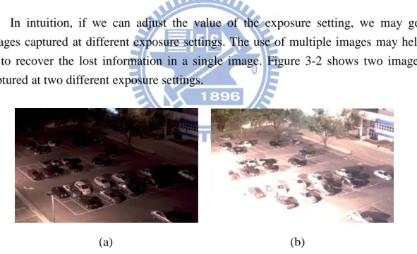
In intuition, if we can adjust the value of the exposure setting, we may get images captured at different exposure settings. The use of multiple images may help us to recover the lost information in a single image. Figure 3-2 shows two images captured at two different exposure settings.

(a) (b)

Figure 3-2 (a) An image with short exposure (b) An image with long exposure

Basically, if we extend the exposure period when capturing an image, we can get more details in the dark areas. On the contrary, if we shorten the exposure period, we may get more details over the very bright areas. Hence, if we can get images captured at different exposure settings and find a way to combine these images together, we will be able to get an image with more details. With images of improved quality, we will be able to achieve more robust performance in vacant parking space detection.

3.1.2. C

OMBINATION OF

C

AR

-

DRIVEN AND

S

PACE

-

DRIVEN

M

ETHODS

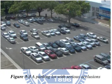
Because of the occlusion problem and the perspective distortion in a large-scale parking lot, the traditional car-driven methods cannot be directly applied to vacant parking space detection without modification. In Figure 3-3, we show a parking lot with the presence of serious occlusions.

Figure 3-3 A parking lot with serious occlusions

However, car-driven detectors can perform very well over images with complicated backgrounds or images with changes of illumination. Hence, we aim to make some modifications over car-driven detectors to make them also suitable for parking lots with serious occlusion. In our approach, we try to combine together the car-driven approach and the space-driven approach. In the car-driven approach, we check car-level data over the parking spaces, as shown in Figure 3-4(a). On the other hand, in the space-driven approach, we check pixel-level or patch-level data over the parking spaces, as shown in Figure 3-4(b). In comparison, in our approach, we treat the detection unit as a set of composing surfaces. The ground plane of a parking space is made of ground surface while a car is made of several surfaces, as illustrated in (c) and (d) of Figure 3-4.

(a) (b)

(c) (d)

Figure 3-4 (a) Car-level data. (b) Patch-level data (c) Ground surfaces (d) Car surfaces According to the regularity of occlusion patterns in the parking lot, we can detect vacant parking spaces by determining the labels of each surface. Each parking spot can be thought as a cubic consisting of six surfaces and some of these surfaces are shared by neighboring parking spaces. Figure 3-5 shows the six surfaces of a parking space and Figure 3-6 shows various kinds of patterns at each of these surfaces.

Figure 3-6 Possible patterns at each surface of the parking space

As shown in Figure 3-6, there are fourteen kinds of surface patterns in total. Here, each surface pattern is labeled by its surface name and the index of the pattern, such as T_1, G_1, or S_1. Based on the observed surface patterns in the parking area, we use the Hierarchical Bayesian Framework (BHF) proposed in [15] to represent the parking block, as illustrated in Figure 3-7.

There are three layers in the BHF framework, which are observation layer, label layer, and scene layer. In the observation layer, we treat the whole parking lot as a set of surfaces, with some of these surfaces being shared by neighboring parking spaces. In the label layer, a node represents the label of a surface. In the scene layer, a node indicates the parking status of a parking space, such as “parked” or “vacant”.

With the BHF framework, Figure 3-8 illustrates the inference flow of our detection procedure. At the observation layer, we treat the whole parking lot as a set of surfaces and compute at each surface the probability of every possible label. Once the probabilities of every possible level are obtained, we compute the probability of each parking hypothesis by using the information passed from the scene layer. Here, a hypothesis indicates a combination of the parking statuses of the parking spaces in the parking lot and we compute the probability of each hypothesis individually. Finally, the hypothesis with the highest probability value will be chosen and that hypothesis indicates the deduced parking space statuses.

3.2. D

ETECTION

A

LGORITHM OF THE

P

ROPOSED

S

YSTEM

In the previous section, we have introduced the basic concept of the proposed vacant parking space detection system. In this section, we will introduce the detection procedure of our system. In Figure 3-9, we show the detection flowchart of the proposed method. First, we design an image-capture process that captures images with different exposure settings. After that, these multi-exposure images are fused to obtain an image with improved quality. With the fused images and some 3D scene information, we obtain the image patch of each surface in the parking area. By extracting features from each image patch and matching them with respect to the pre-trained data, we can estimate the probability of each pattern label. Finally, by computing the probabilities of all parking hypotheses, we can deduce the most likely parking statuses of the parking lot.

3.2.1. I

MAGE

C

APTURE

S

YSTEM

To get multi-exposure images, we use the AXIS M1114 IP camera which can adjust the exposure values of the captured images. Figure 3-10 shows the camera settings of this camera. By using the Software Develop kit (SDK) provided by AXIS, we design an image capture system which repeatedly captures images at different exposure settings, as illustrated in Figure 3-11.

Figure 3-10 The camera settings of AXIS M1114, where the setting of exposure value is marked by

Figure 3 -11 Details of our image capture system

In our image capture system, we gradually increase the value of the exposure setting from a small initial value. When the exposure value reaches the pre-selected upper bound, its value is reset to the initial setting again. With this repetitive process, we can get a bag of multi-exposure images at each moment and only need to wait an exposure period to get an updated bag of multi-exposure images. In our system, the longest exposure period is chosen to be around 3 seconds and we select three different exposure values: EV=10, 50, and 90. Figure 3-12 shows three images captured with EV=10, EV=50, and EV=90, respectively.

(a) (b) (c) Figure 3-12 (a) The captured image with EV=10 (b) The captured image with EV=50

(c) The captured image with EV=90

3.2.2. E

XPOSURE

F

USION

Once we have gotten a bag of multi-exposure images, we can use the high dynamic range imaging (HDR) technique proposed in [13] to recover the scene information. In [13], the authors measure the quality of each pixel based on a set of multi-exposure images and generates the final result by combining multi-exposure images with different weighting maps. By using contrast, saturation and

well-exposedness as the factors, the authors can automatically compute the weighting maps. Eq. 3-1 and Eq. 3-2 are the proposed formulas, where C, S, and E indicate the contrast factor, the saturation factor and the well-exposedness factor, respectively.

C

 , S_{, and} E _{indicates the corresponding weightings. W is a weighting map,} (i,j) is the pixel index, and k is the k-th image.

W_{i j k,} (C_{,i j k})C  (_{i j k}S_, )S  (_{i j k}E_, E) Eq. 3-1 After normalization, 1 , _{, ' ,} ' 1 [ ] N ij k _{ij k ij k} k W W W    



By combining multi-exposure images and their weighting maps based on the above formulas, we will get an image of improved quality. In Eq. 3-3, R denotes the recovered image after the exposure fusion.

, , 1 N ij ij k ij k k R W I   



Unfortunately, due to the dramatic variation of the weighting maps, the fused image may have undesired halos around edges. To overcome this problem, the authors use the image pyramid decomposition. Here, the input images are decomposed into a Laplacian pyramid. The fusion process is performed at each level of the pyramid. Finally, the resulting pyramid is used to reconstruct the fused image. Figure 3-13 shows the pyramid-based procedure of exposure fusion and Figure 3-14 shows a result of this method.

In Figure 3-15, we show a fusion result of these three images in Figure 3-12. It is apparent that the fusion image can capture more details if compared with the original images without fusion. The comparison of the gradient magnitude between the fusion image and the original image (EV=50) is shown in Figure 3-16.

(a) (b) Figure 3-14 (a) An Image sequence and its weighting maps (b) The fusion result

Figure 3-15 The fusion result of the images in Figure 3-12

(a) (b)

Figure 3-16 Comparison of gradient magnitudes between the original image and the fused image

(a) The gradient magnitude image of the original image (b) The gradient magnitude image of the fused image

3.2.3. F

EATURE

E

XTRACTION

To analyze each surface of the parking area, we get image patches from the corresponded parking spot first. With the pre-known 3D scene information, we know the position and region of every surface in the real world by using the calibration matrix between the real world and the camera images. In Figure 3-17, we show the six

surfaces and the corresponding image regions of a parking space in the parking lot.

Figure 3-17 The six surfaces and the corresponding image regions of a parking space

Once we get the image region of each surface, we extract features from it. However, due to the perspective distortion of the camera, same surfaces in the 3-D world may appear quite different in the captured image. An example of perspective distortion is shown in Figure 3-18.

Figure 3-18 Image regions of the side surface at four different parking spaces

To deal with perspective distortion, we use the calibration method proposed in [9]. Because surfaces of the same kind would have the same width, length, and depth in the real world, we can normalize image regions at different positions of the image into image patches of the same size, as illustrated in Figure 3-19. In this figure, we transform image regions of the same surface type into normalized image patches of

length “a” and width “b”. In Figure 3-20, we show the normalized patches of the image regions at four different parking spaces in Figure 3-18.

Figure 3-19 Normalization of image regions

Figure 3-20 Normalized image patches of the side surfaces at four different parking spaces After transforming all image regions into normalized image patches, we extract features from them. Since we want our features to be robust and not easily affected by shadows or the changes of illumination, we use the HOG feature proposed in [3] that works well against shadows and the changes of illumination. In [3], the authors propose a robust method for pedestrian detection. The authors’ goal is to find pedestrians in various kinds of images which contain complicated backgrounds. Instead of using pixel value or the gradient value between pixels, the authors measure

the statistics of a larger image region that covers several local cells. Figure 3-21 shows an image patch that consists of many cells.

Figure 3-21 An image patch consisting of many cells

Over the larger image regions, the authors in [3] compute the histogram of oriented gradients at each cell by counting the distribution of gradient magnitudes at a few gradient orientations. However, when an object appears in an image patch, the appearance of the object may be affected by shadows or changes of illumination. To deal with these interferences, the authors group several cells into a block and perform normalization over each block to overcome the changes of illumination and the shadow effect. Figure 3-22 shows the feature extraction process of the histogram of

oriented gradients (HOG) feature. Figure 3-23 shows an image and its HOG features.

Figure 3-22 Extraction of HOG features

(a) (b) Figure 3-23 (a) Original image (b) HOG features

In the HOG feature, the histogram information in all cells are merged together to form a high-dimensional vector. In our case, however, we make a minor modification over this HOG feature. In our case, the cars parked in the parking lot are somewhat different in their brands, types, or the parked position within the parking space. To allow such fluctuations, we further group a few cells together to form super-cells. Figure 3-24 shows an example in which we divide a region of 48 cells into 22 super-cells by adding together the distribution data within each super-cell. After that, we construct the HOG feature based on the distribution data of these four super-cells.

(a)

(b)

Figure 3-24 (a) The definition of super-cell

(b) An example of merging a region of 48 cells into 22 super-cells

3.2.4. D

ISTRIBUTIONS OF

S

URFACE

P

ATTERNS

As mentioned before, we have defined fourteen different kinds of surface patterns. For example, for the top surface, there are two possible patterns: “with a car” pattern and “without a car” pattern. For the side surface, there are four patterns according to the parking status of that parking space and the parking status of the adjacent parking space. Similar to the side surface, there are four possible patterns for the ground surface. On the other hand, the rear surface of a parking space is actually the front surface of the parking space right behind. Hence, there are four possible surface patterns for either the front surface or the rear surface. Figure 3-25 shows these possible patterns of each surface at a parking space.

Figure 3-25 Possible patterns of each surface at a parking space

In our approach, given a set of training data, we use the features extracted from the normalized image patches to train the probabilistic distribution of each possible surface pattern. With the trained distributions, we will be able to estimate for any given patch the likelihood value of being a certain kind of surface pattern.

3.2.5. I

NFERENCE OF

P

ARKING

S

TATUSES

Because of the geometric structure of our parking lot, we divide our parking lot to three major blocks and we do the labeling of each block independently. Figure 3-26 shows each block of our parking lot.

Within each parking block, we build a Hierarchical Bayesian Framework (BHF) model to infer the parking statuses of that parking block, as illustrated in Figure 3-27. The scene layer denotes the parking statuses of all parking spaces, the label layer denotes the label of each surface, and the observation layer denotes the features extracted from each surface.

Figure 3-27 The BHF model of a parking block

Given a hypothesis about the parking statuses of the parking lot, there would be one corresponding surface pattern for each surface in the parking block. Hence, as we match a hypothesis with the observed information from the observation layer, we measure the probabilistic value of being that corresponding surface pattern for each surface. By calculating the product of the probabilistic values of all surfaces in the parking block, we obtain a score that indicates how likely this hypothesis is true. By comparing the scores of all possible hypotheses, we pick the hypothesis with the largest score and deduce the parking statuses accordingly. In Figure 3-28, we illustrate the matching process of our BHF model.

Figure 3-28 The inference process of our proposed method

If we only use the local information passed from the observation layer for inference but do not use the global parking hypotheses at the scene layer, we may obtain some labeling results that conflict with each other. With the inclusion of the scene hypothesis, the solution space is limited to the space of feasible labeling results. Hence, the whole detection process becomes more stable and more accurate.

Our labeling process is equivalent to maximizing the following formula: * arg max ( | ) L L L L S S  p S O Eq. 3-4

In our case, there is a one-to-one mapping fbetween SL and NL, as shown below.

( )

L L

N  f S

,SL Eq.3-5

To find the SL* is the same as to find the corresponding NL* and Eq. 3-4 can be

rewritten as * arg max ( | ) L L L L N N  p N O Eq.3-6 arg max[ ( | ) ( )] L L L L N p O N p N 

Here, we assume SL follows a uniform distribution. Hence, with a one-to-one mapping

between SL and NL,NL is also uniformly distributed and we have

* arg max[ ( | ) ( )] L L L L L N N  p O N p N arg max[ ( | )] L L L N p O N  1 1 2 2 arg max[ ( | ) ( | ) L L L L L N p O N p O N    1 1 ( k L| k L) ( kL| kL)] p O  N  p O N  

Finally, SL* is our detection result of the parking block. By applying the same

procedure to the other two parking blocks, we can estimate the parking statuses of the whole parking lot.

3.3. T

RAINING

P

ROCESS

In Figure 3-29, we show the possible surface patterns at a parking space. By using the features discussed above, we can train the distribution for each surface pattern in advance. Taking the top surface as an example, we collect from the training images a lot of HOG features belonging to the label “T_1” and a lot of HOG features belonging to the label “T_2”. These two kinds of HOG features will form two different distributions in the feature space. Because the dimension of the feature vectors are very large, we adopt the Linear Discriminant Analysis (LDA) method to lower the feature space down to the three-dimensional space and compute the probabilistic value of each label in this 3-D space.

Figure 3-29 Labels according to different patterns of surfaces

Different from Principal Component Analysis (PCA), which lowers down the dimension of data by directly projecting the data points to the subspace formed by the major eigenvectors, LDA finds the subspace that can lower down the dimension of data while preserving the diverseness of data classes. An example is shown in Figure 3-30 to illustrate the difference between PCA and LDA. We can easily see that the data projected by LDA preserves more information without destroying the difference between classes.

Suppose x indicates the original data and there are C classes. Let ibe the mean

vector of the class i,  _{be the mean vector of total data, and M}i be the number of

samples within the class i. Suppose there is a projection matrix PT _{that projects the} data x to y. The between-class scatter matrix and the within-class scatter matrix can be expressed as below.

Within-class scatter matrix: 1 1 ( )( ) i M C T T w j i j i i j S P x  x  P   



Between-class scatter matrix:

1 ( )( ) C T T b i i i S P     P  



The LDA method aims to minimize the within-class scatter matrix while maximizing the between-class scatter matrix. This idea can be formulated as

| | ( ) | | t b t w P S P J P P S P  Eq. 3-9

To maximize the above equation is the same as to solve the eigenvectors of Eq.3-7.

b w

S PS P Eq. 3-10

Finally, by picking the N eigenvectors that corresponding to the N largest eigenvalues, we can reduce the dimension of the original data while preserving the characteristics of the class distributions.

For the top surface, Figure 3-31 shows the distributions of the two possible surface patterns "T_1" and "T_2". Distributions of the other surface patterns are shown in Figure 3-32. Moreover, in our experiment, we model the distribution of each surface pattern as a gaussian function.

Figure 3-31 Distributions of the "T_1" and "T_2" patterns of the top surface

3.4. I

MPLEMENTATION

D

ETAILS

In our detection procedure, once we get an HOG feature from an image patch, we compute the probabilistic value of this feature with respect to every possible surface pattern. In fact, we can save the computations by using the 3D scene information in advance. For an example, if we want compute how likely the HOG feature belonging to the top surface, we only need to consider the cases of “T_1” and “T_2”. This would take fewer computations on the detection process.

Moreover, in the detection step, as we make our decision for a parking block, we have to consider all possible parking hypotheses of the parking block. Unfortunately, the number of parking hypotheses grows exponentially with respect to the number of parking spaces in the parking block. In our experiments, there are as many as twenty-six parking spaces in a parking block. This leads to about seventy million hypotheses! Hence, in our work, we further divide a parking block into two rows and do the detection for the front row first. With the detection result of the first row, we detect the parking statuses of the second row afterward. Figure 3-33 illustrates this approach. Although this approach may sometimes generate detection errors, it saves a lot of computation time without sacrificing too much accuracy in detection.

Figure 3-33 Row-wise detection procedure

If the size of the parking lot is too big and there are still too many parking spaces in a single parking row, we can further reduce the computation time by considering only a few surfaces that are neighboring to the present parking space for inference. It would take much less time in detection and does not deteriorate the overall performance too much. Some experimental results of this simplified approach will be shown in Chapter 4.

Moreover, although we have considered the fluctuations of surface patterns caused by the variations of car brands, car types, or the parked position within the parking space, there are some other situations that complicate the problem. Figure 3-34 shows two cases that the cars park too inside or too outside of the parking space. This may lead to incorrect inference. To deal with this problem, we sample the HOG feature at three different positions within the parking space and take the largest probabilistic value for inference. An example is shown in Figure 3-35, which samples the front surface at three different locations. With this approach, we can handle the dramatic fluctuation of parking position effectively without affecting the detection result of the other parking spaces.

(a) (b)

Figure3-34 (a) A car parked too inside of the parking space (b) A car parked too outside of the parking

space

Chapter 4.

E

XPERIMENTAL

R

ESULTS

In this chapter, we will show some experiment results of our proposed method. Before the introduction of our experiments, we mention some specifications of the parking lot in our experiments. In this parking lot, there are three major blocks and there are seventy-two parking spaces in total. Figure 4-1 shows an image of the parking lot and the detection regions of the three parking blocks.

Figure 4-1 (a) An image of the parking lot. (b) The corresponding detection regions.

To evaluate the performance of our system, we calculate positive rate (FPR), false negative rate (FNR), and accuracy (ACC), which are defined as below.

number of parked spaces being detect as vacant FPR=

total number of parked spaces Eq.4-1

number of vacant spaces being detect as parked FNR=

total number of vacant spaces Eq.4-2

number of correct detection in both parked and vacant spaces ACC=

In our experiment, we divide the whole day into two periods: day period (5:00~19:00) and nigh period (19:00~5:00). We will demonstrate the performance of each period separately. Since there is almost no change of parking status during the early morning period (0:00~5:00), we do not take that period into account. Moreover, the multi-exposure preprocessing is only used during the night period and there is no need to use the multi-exposure preprocessing during the day period.

Table 4-1 shows our experimental results for the day period which includes the performance of each parking block and the performance in a normal day, a sunny day, a cloudy day, and a rainy day, respectively. In Figure 4-2, we show image samples that are captured in these four different types of weather.

Table 4-1 Day period performance of the proposed method

(a) (b)

(c) (d)

Figure 4-2 Image samples captured in (a) normal day, (b)sunny day, (c) cloudy day, and (d)rainy day #of tested spaces Proposed method

vacant parked total FPR FNR ACC

Normal 4937 7519 12456 0.0028 0.0097 0.9945 Sunny 8259 3405 11664 0.0012 0.0115 0.9915 Cloudy 5774 6250 12024 0.0022 0.0002 0.9988 Rainy 3668 6916 10584 0.0078 0.0049 0.9932 Block_1 6857 10017 16874 0.0012 0.0004 0.9986 Block_2 8701 8173 16874 0.0020 0.0064 0.9955 Block_3 7080 5900 12980 0.0034 0.0145 0.9905

As aforementioned, there are four major problems in daytime vision-based parking space detection: occlusion effect, shadow effect, perspective distortion, and fluctuation of lighting condition. The following experiments will demonstrate that our method can deal with these problems effectively. In Figure 4-3, we show the detection result under different kinds of shadowing. With the use of the modified HOG feature, our method can deal with the shadow problem effectively.

(a) (b)

(c) (d)

(e) (f)

Figure 4-3 (a)(c)(e): Images with shadow effect (b)(d)(f): The corresponding detection result Besides shadow effect, our proposed method can also deal with the fluctuation of lighting condition. Some examples are shown in Figure 4-4. Although there are dramatic changes of colors in these images, our algorithm still works very well. This is because we have used the gradient information in our system which is less affected

by the change of illumination.

(a) (b)

(c) (d)

(e) (f)

Figure 4-4 (a)(c)(e): Images with different lighting condition (b)(d)(f): The corresponding detection results Moreover, for the comparison with other algorithms, we test Dan’ method in [10], Wu’s method in [11], Huang’s method in [6], and Huang’s method in [15] over the dataset released by Huang in [15]. For this dataset, there are five rows of parking spaces in the parking lot and there are forty-six parking spaces in total. Here, Row 1 denotes the bottom row and Row 5 denotes the top row. Seq_1 is an image sequence captured in a normal day, Seq_2 is an image sequence captured in a sunny day, and Seq_3 is an image sequence captured in a cloudy day. Figure 4-5 shows some examples of these three image sequences and Table 4-2 lists the experimental results.

If compared to the performance of Huang’s work in [15] which achieves the best performance among all algorithms, our method achieves comparable performance in the day period. However, Huang’s method is much more complicated and needs some extra information such as the angle of the sunlight direction. Besides, our system outperforms Huang’s in the cloudy day case. This is because Huang’s method relies heavily on the color information. This makes his system less accurate in a cloudy day.

Table 4-2 Comparisons of day period performance

#of tested spaces Dan [10] Wu [11]

vacant parked total FPR FNR ACC FPR FNR ACC Seq_1 498 4470 4968 0.0307 0.5748 0.9153 0.0111 0.7115 0.9193 Seq_2 278 4644 4922 0.0101 0.7061 0.9537 0.0016 0.7837 0.9577 Seq_3 206 4716 4922 0.0073 0.6524 0.9703 0.0018 0.7012 0.9739 1st&2nd 649 6757 7406 0.0179 0.5641 0.9381 0.0068 0.6960 0.9377 3rd&4th 98 5376 5474 0.0059 0.6933 0.9840 0.0028 0.6933 0.9871 5th 235 1697 1932 0.0366 0.7554 0.8764 0.0024 0.8240 0.8982

Huang [6] Huang [15] Proposed method

FPR FNR ACC FPR FNR ACC FPR FNR ACC

0.0004 0.1690 0.9827 0.0004 0.0081 0.9988 0.0029 0.0361 0.9938 0.0002 0.2626 0.9850 0.0024 0.0324 0.9959 0.0015 0.0396 0.9963 0.0042 0.1019 0.9917 0.0040 0.0437 0.9943 0.0009 0.0049 0.9990 0.0025 0.1770 0.9823 0.0019 0.0233 0.9962 0.0025 0.0231 0.9957 0.0009 0.3163 0.9934 0.0015 0.0306 0.9980 0.0013 0.0000 0.9987 0.0006 0.1373 0.9829 0.0065 0.0172 0.9922 0.0000 0.0638 0.9922 (a) (b) (c)

Figure 4-5 Three images captured under different weather conditions in Huang’s dataset [15] (a)

For the night period, the multi-exposure pre-processing is included in our detection procedure. In addition, before the fusion stage, we apply a median filter to the multi-exposure images with the 33 mask size for the EV=10 setting, the 55 mask size for the EV=50 setting, and the 77 mask size for the EV=90 setting. This filtering process can greatly reduce the image noise that occurs when capturing images in a dark environment. However, the head light of moving cars in the parking lot and the lamps in the parking lot may also cause dramatic fluctuation of lighting condition in the parking lot. Even though these conditions are not specially considered in the design of our system, our system can still roughly handle these cases with the help of the modified HOG feature. In Table 4-3, we demonstrate the performance of our system over the night period when there is no moving car in the parking lot. The comparison with Wu’s method [11] is also shown in Table 4-3. Some images and their detection results of these night period sequences are shown in Figure 4-6.

(a) (b)

(c) (d)

(e) (f)

Table 4-3 Night period performance of the proposed method

#of tested spaces Wu [11] Proposed method vacant parked total FPR FNR ACC FPR FNR ACC Seq_1 4592 3112 7704 0.1520 0.1021 0.8777 0.0135 0.0294 0.9770 Seq_2 4659 2631 7200 0.1281 0.0989 0.8904 0.0049 0.0282 0.9803 Seq_3 4540 2588 7128 0.1565 0.1260 0.8629 0.0232 0.0172 0.9806 Block_1 4480 3476 7956 0.0630 0.1313 0.8986 0.0147 0.0221 0.9811 Block_2 5051 2905 7956 0.1535 0.1026 0.8788 0.0048 0.0123 0.9904 Block_3 4170 1950 6120 0.2821 0.0928 0.8469 0.0256 0.0434 0.9623 (a) (b)

Figure 4-7 (a)(b) Night period detection with moving cars in the scene

Row 1: image samples with EV=10, EV=50, and EV=90 Row 2: Fused images and the corresponding detection results