使用晶片參考資料庫及簡易學生T檢定之基因表現晶片預測分析

國 立 交 通 大 學

統計學研究所

碩 士 論 文

使用晶片參考資料庫

及簡易學生 T 檢定之基因表現晶片預測分析

Prediction analysis for gene expression microarrays

using a reference set and simple t test

研 究 生：陳淑慎

指導教授：黃冠華 博士

使用晶片參考資料庫

及簡易學生 T 檢定之基因表現晶片預測分析

Prediction analysis for gene expression microarrays

using a reference set and simple t test

研 究 生：陳淑慎

Student: Shu-Shen Chen

指導教授：黃冠華

Advisor: Dr. Guan-Hua Huang

國 立 交 通 大 學

統計學研究所

碩 士 論 文

A Thesis

Submitted to institute of Statistics College of Science

National Chiao Tung University in Partial Fulfillment of the Requirements

for the Degree of Master

in Statistics July 2009

Hsinchu, Taiwan, Republic of China

使用晶片參考資料庫

及簡易學生 T 檢定之基因表現晶片預測分析

研究生：陳淑慎 指導教授：黃冠華 博士

國立交通大學統計學研究所

摘要

Prediction analysis for gene expression microarrays using a

reference set and simple t test

Student: Shu-Shen Chen Advisor: Dr. Guan-Hua Huang

Institute of Statistics

National Chiao Tung University

ABSTRACT

We collect published Affymetrix GeneChip HGU-133A arrays from AE(ArrayExpress) and GEO (Gene Expression Omnibus), and select normal control arrays to build up a reference set. R package RefPlus is used to preprocess new target arrays without re-preprocessing them along with the reference set together again. We pick up some “representative” genes through the idea of bar code and build up six classifiers by simple t tests. We then compare the classification abilities between our six classifiers and PAM.

誌謝

Contents

Abstract (in Chinese) i

Abstract (in English) ii

Acknowledgements (in Chinese) iii

Contents iv

List of Figures vi

List of Tables vii

1. Introduction 1

2. Literature Review 3

2.1 Affymetrix GeneChip array……….……….3

2.2 Microarry Retriver………3

2.3 Quality Control……….4

2.4 justRMA, our preprocessing function………....5

2.5 Testing Dataset………..7

2.6 The view of multiple modes……….7

2.7 The idea of gene expression cut-off form from bar code………..8

2.8 Classification……….8

2.9 Prediction analysis for microarrays (PAM)………9

3. Materials and Methods 11

3.1 To seek and find a reference set from publicly available databases……….11

3.1.1 Use Miscroarray Retriever to search and download arrays……….11

3.1.2 Choose normal control arrays………11

3.1.3 Perform chips’ quality assessment……….11

3.2 To preprocess our reference set and classify arrays by tissues………..12

3.4 Six classification rules………13

3.4.1 Method 1 (corrected by the reference set and training groups)……….14

3.4.2 Method 2 (corrected by the reference training set)………15

3.4.3 Method 3 (no corrected)……….16

3.4.4 Method 4 (corrected by multiplying the standard deviation of the jth probe in the reference set)………..16

3.4.5 Method 5 (corrected by multiplying the standard deviation of the jth probe in the reference set and dividing the standard deviation of the jth probe in the training group)………..17

3.4.6 Method 6 (corrected by dividing the standard deviation of the jth probe in the reference set)………...17

3.5 To obtain the list of genes with multiple modes from the idea of bar code………....18

3.6 Do classification procedure again (Method1~Method6) with multiple-mode genes.19 3.7 Classify testing set by PAM………19

4. Result 20

5. Conclusion and discussion 22

List of Figures

Figure 2.1 The design of probes for Microarray HGU133A chip………26

Figure 2.2 The distribution of expression intensity from different genes………26

Figure 2.3 The idea of cut-off point choosing………..27

Figure 3.1 The distributions of those delete arrays over all 2445 arrays in four quality

assessment metrics. The red dots represent all deleted data………28

Figure 3.2 Summary of different combinations of “n” and “adjust” when fitting smoothing

density function using R function density(n,adjust), different color lines represent different smooth curves with various “adjust” values.……….…….29

Figure 4.1 The histogram of the mean expression value of all genes for reference set…...30

Figure 4.2 The histogram of the sample standard deviation of expression value for all

genes in reference set………...….31

Figure 4.3 The histogram of absolute different value of mean expression between disease

group in testing set and reference set………32

Figure 4.4 The histogram of absolute different value of mean expression between

non-disease group in testing set and reference set………..33

Figure 4.5 Summary of classification results, where a point means we classify successfully

once and green points and black points were the results from doing simple t-test by 5005 multiple-mode genes and by all 22283 genes respectively.…...34

List of Tables

Table 3.1 Summary of QC step………35

Table 3.2 The distribution of the number of arrays in each tissue type………35

Table 3.3 The number of arrays in each tissue type……….36

Table 4.1 The results of the leave-one-out cross validation, using various classification

1. Introduction

Microarray is a useful design to simultaneously measure the expression values of many thousands of genes in a particular species or tissue. Nowadays, Microarray is widely used in many areas of biomedical research and Affymetrix GeneChip platform is selected in most time. There are millions of probes on an Affymetrix array. Two kinds of probes with length of 25 nucleotides are designed. One is “prefect match (PM)” probe which perfectly matches its target sequence. Another one is “mismatch (MM)” probe which is different with its paired perfect match in the middle base (13th) of probe sequence. Mismatch is created to detect the nonspecific binding because its paired perfect match may be hybridized to nonspecific sequence. So a paired PM and MM is called a “probe pair” and there are 11-20 probe pairs to represent a gene typically. Because of this special design, preprocessing Affymetrix expression arrays usually involves three main steps, which are background adjustment, normalization, and summarization. When we have a large set of Affymetrix arrays, we should preprocess them together. This is a necessary step before we use and analyze the information included in those arrays. At all times, we will refresh our database and compare all arrays that we have, old and new. Each time we add a new data to our database, we need to re-preprocess all arrays together again. This is a big work and is inconvenient. So, we want to find a general reference database that contains arrays created through most of tissue types that we usually use. Then, basing on the information of the reference dataset, we can preprocess our new arrays without re-preprocessing new and old arrays altogether.

Also, reference dataset can be used to improve the accuracy of classifying new data. We build up 6 different kinds of classifiers that incorporate our created reference set to increase their generalization ability of classification. The major difference between our classifiers and those existing classifiers is the number of variables (genes) used for classification. We choose all genes (or all “multiple-mode” genes) to build up our classifiers, instead of

choosing some differentially expressed genes as done in existing methods. Simple t-test is then applied to all chosen genes for classification. It is found that our classifiers perform as well as those existing complicated rules (e.g., PAM (Tibshirani et al.,2002)).

2. Literature Review

2.1. Affymetrix GeneChip array

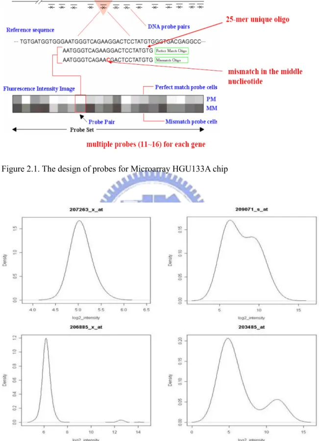
Affymetrix GeneChip array is one kind of microarrays that is used to high throughput assay for measuring the expression levels of many thousands of gene transcripts in one particular cell type or tissue at the same time. There are two main aspects of experimental design of microarrys. One is target design that mRNA samples allocate to the slides. The other is probe design that sequences print on the array. The technology of Affymetrix GeneChip include RNA extraction, RNA labeling, hybridization, washing and staining. It takes advantage of hybridization properties of nucleic acid. “Probe” is a combination of complementary molecules attached to a solid surface for our “target” that is the specific nucleic acid transcripts of interest presented in the sample and we used it to measure how much quantity of “target”. Millions of probes with a general length of 25 nucleotides are produced on an Affymetrix array. Affymetrix GeneChip probe design show in Figure2.1(Affymetrix GeneChip user guide).

Pixel intensity values of the arrays are calculated using peculiar instruments by Affymetrix after RNA samples were prepared, labeled, hybridized to an array with millions of probes and array was scanned. Based on these probe-level intensities values, intensity values for each probe are computed and stored in a CEL file (contains probe cell intensities). Those CEL files of HG-U133A raw data are our targets of data collection.

2.2. Microarray Retriver

Microarray retriever is a web-based tool for searching and a large scale retrieval of public microarray data (Ivliev, 2008). Meta-analysis studies in which expression data is combined with multiple individual studies are using widely since it is useful for discovery of genes disproportionately overexpressed in specific tissue types, construction of robust

high-resolution gene coexpression networks and identification of rhythmically expressed genes for example. And it may improve the interpretation of new experimental studies by comparison with data that already publicly available. Microarray Retriever (MaRe) facilitates meta-analysis through searching and collecting data retrieval from two major public microarray repositories that are ArrayExpress (AE, European Bioinformatics Institute) and Gene Expression Omnibus (GEO, National Center for Biotechnology Information). MaRe allows us to search these two repositories for experiments with accession numbers, species, array platform, authors, date of submission and keyword search terms. It resolves the hurdle of retrieving the relevant datasets from microarray data repositories and saves the time of manual and sequential download data from the web or ftp sites of AE and GEO.

2.3. Quality Control

We perform a series of QC (quality control) metrics that is used to check all arrays that we colected have been hybridized correctly and the sample quality of arrays is acceptable. We use the function “qc” in the R package “simpleaffy” to do the procedure of QC (ACBB & Wilson et al.). That was contained some general QC statistics and standard QC functions recommended for Affymetrix arrays. And we choose this function qc is because of it can be called with raw data (in the AffyBatch object) and that let we can calculate the value of scale factors. To assess the quality of data generated in our database, we consider four out of the metrics (Scale factor, Background level, 5'/3' ratios for GAPDH and beta-actin and Proportion of transcripts called present) in the qc function. Details as the follow:

1. Average background: The value of average background is the level of background noise for each chip which is experiencing that shows a considerable amount of variation. 2. Scale factor: The level of scaling applied to an array when normalized using

3. 3’ to 5’ ratios for β-actin and GAPDH: the value of 3’/5’ ratios is the ratio of the 3’ expression to the 5’ expression for some quality control genes.

4. Percent present calls: the number of genes called present (% present calls) is representing the percentage of probesets called present on an array and shows a broad spread in values across the whole experiment (27-57%) there is good general agreement between samples in each replicate group and between each experimental condition. The criteria of these four metrics is

1. Scale factors should be within 6-fold, 4-fold, and 3-fold of each other stepwisely. 2. Those values of averages background should be smaller than 300.

3. The value of actin3/actin5 should not exceed 3 and the value of gapdh3/gapdh5 should not exceed 1.25.

4. Those values of percent present should be not less than 20%.

2.4. justRMA, our preprocessing function

Since many systematical biases from different sources in microarray experiments the preprocessing procedure of data becomes more necessary and more important. To get a correct intensity value that represents the abundance of mRNA instead of an uncertain brightness biased by other sources is the goal of preprocessing. RMA is one preprocessing method of most popular preprocessing methods.

“justRMA” is a function of R package named “affy”, that can read .cel files and compute the RMA (robust multi-array average) expression measure without using an AffyBatch. “rma” is a function of the affy package that be considered as the canonical implementation of RMA and converts an AffyBatch into an ExpressionSet during the RMA calculation. Both of justRMA and rma do the same expression estimates. So compare to the function “rma”, “justRMA” is a better option for the user of function “rma” with a really huge dataset that need to process together or struggling with memory problem. We use justRMA

instead of rma in our preprocess step. And RMA (the Robust Multichip Average) methodology consists of three steps that are a background adjustment, quantile normalization and summarization (Irizarry et al., 2003). RMA methodology only use PM (perfect match) probes since MM (mismatch) may detect not only non-specific binding and background noise but also the transcript signal just like the PM probe and that is not always appropriate to subtracting the MM intensity from the PM intensity as the way of correcting for background noise and non-specific binding. Convolution background correction method in the background adjustment of RMA is assumed that the expression value of each PM probe (PMijg) combine with background intensity caused by optical and nonspecific binding ( bgijg ) and signal intensity ( sijg ), as follow:

, ijg ijg ijg

PM =bg +s i=1, , ,_L I j=1, , ,_L J g =1, ,_L G

And the background corrected probe intensities is (B PMijg)=E s( ijg |PMijg) , where we assume that bgijg is distributed normal and s is distributed exponential. There are ijg many obscuring sources of variation involved during the process of carrying out the microarry experiment involves multiple arrays, such as physical problems with laboratory conditions, hybridization reactions, labeling, arrays and scanner difference. So proper normalization is necessary for comparing measurements from different arrays that implying different tissues. The step of summarization is to combine those probe intensities that pass through background adjusted and normalized to a single measurement that estimates the expression value for each gene. Then the summarization of RMA is using the median polish algorithm that assume the value of the background corrected, normalized and took a log of PM intensities ( (T PMij)) is the combination of the log scale expression value on array i (e ), the log scale affinity effects for probe j (i a ), and error term (j εij), the formula

is (T PMij)= +ei aj+ . εij

We use the estimate of e as the log scale measure of expression. i

2.5. Testing Dataset

We choose our testing dataset that is not in our reference training set. And for comparing our reference training set to the datasets of thesis of “bar code”, we choose our testing dataset through the thesis of “bar code”. We choose a dataset with 159 arrays from a breast cancer study (GEO identifier is GSE1456) (Pawitan et al., 2005). All 159 arrays in this study did not include our reference training set. Those samples was been included at the Karolinska Hospital from 1 January 1994 to 31 December 1996(n=524) and excluded to sample size 159 (n=159). In the end, there are 38 poor prognosis samples and 121 good prognosis samples in this dataset.

2.6. The view of multiple modes

Typically we assume the expression intensity for each gene is ( )f , where cases and

controls separately follow f( )μ₁ and f( )μ₂ with different means, and all genes follow

the same distribution ( )f that usually be normal, mixture of normals, or lognormal. But

in fact each gene has its own distribution since the “probe effect” is large. We can find this from the following graph that are some probability density functions of the expression intensity values which has been taking log2 for different genes on the same array. There are one mode distribution, two close modes distribution, more than two modes distribution, and two separate modes distribution in Figure 2.2(Zilliox and Irizarry, 2007).

Since it is expected that any given gene will be expressed only in some tissues, multiple modes should be observed. And based on those published studies of gene expression, we think most genes should only have one mode in its probability density function and most

genes are unexpressed in most tissues. So we assume that the lowest intensity mode of those genes with multiple modes distribution is due to a lack of expression. Then we determined the expression intensity distribution for each gene through collecting the raw data from published repositories web and simulation it.

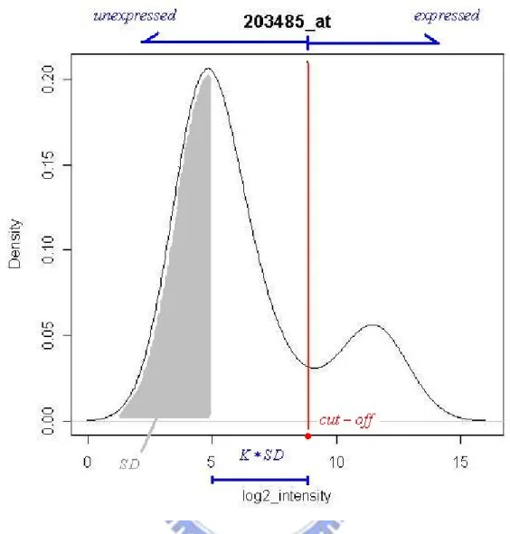
2.7. The idea of gene expression cut-off form from bar code

Since the probability density function of gene expression intensity value have multiple modes, we can simulate the “unexpressed” intensity from the lowest intensity mode and the “expressed” intensity from the others. This idea is from “A gene expression bar code for microarray data” (Zilliox and Irizarry, 2007). The modes were computed and we considered that the mode with the smallest location is the expected intensity of an unexpressed gene. Expression distribution from 0 to the lowest intensity mode used to estimate the standard deviation of unexpressed genes. Then we selected a constant K and set the genes expressed in tissues where the log expression estimates were K standard deviations larger than the unexpressed mean. We show the idea in Figure 2.3.. If we want to simulate a set of microarray gene expression generating intensity value data, we can simulate unexpressed intensities from the empirical distribution on the left of the cut-off and expressed intensities from the empirical distribution on the right of the cut-off. And we can use this idea to choose those genes with differentially expressed.

2.8. Classification

Class comparison, class discovery, and class prediction are most common types of microarray data analysis. Classification is one of the methods of class prediction. To assign observational units to classes on the basis of variables describing/characterizing those observations is the task of classification. In classification, the classes are predefined and we understand the basis for the classification from a set of labeled observations

(training/learning set), then use this information to predict the class of future observations. In fact, we get the gene profiles, find function f that maps the data matrix of gene expression to classes, then get the predict class. Linear and quadratic discriminate analysis (LDA, QDA), k-nearest neighbor (KNN), and classification and regression tree (CART) are some methods for class prediction. These methods of classification are usually choosing some finite variables (less than 1,000 or smaller than size of training set) to develop the classification rule since it is not reasonable for fit when the number of variables is bigger than the sample size of training dataset. But our goal is to find a classifier with high generalization ability through using as much as possible variables that we can get from the training data generalize to predict a new example (Bittner et al., 2000).

2.9. Prediction analysis for microarrays (PAM)

Prediction analysis of microarrays (PAM) is a statistical technique for class prediction using gene expression data by using shrunken centroids. The method of nearest shrunken centroids identifies subsets of genes that best characterize each class. This technique is general and can be used in many other classification problems (Tibshirani et al.,2002).

This method computes a standardized centroid for each class that is the average gene expression for each gene in each class divided by the within-class standard deviation for that gene. And nearest centroid classification compares the gene expression profile of a new sample to each of those class centroids then set which class with centroid that is closest to in squared distance as the predicted class for that new sample. Then after “shrink” each of the class centroids toward the overall centroid for all classes by the amount that we call the threshold is the difference between nearest centroid classification and the Nearest shrunken centroid classification which is used in PAM. This shrinkage that consists of moving the centroid towards zero by threshold that means to set it equal to zero if it hits zero. Then the new sample is classified by the usual nearest centroid rule using the

shrunken class centroids. We can get two advantages from shrinkage, one is that can make the classifier more accurate by reducing the effect of noisy genes and the other one is to select genes automatically. Since when a gene is shrunk to zero for all classes hat means we should eliminated that gene from the prediction rule. In other words, if a gene is set to zero for all classes except one then we know that high or low expression for that gene in that class. So we want to compare the generalization ability of PAM and our classifiers.

3. Material and Methods

3.1 To seek and find a reference set from publicly available databases

3.1.1 Use Microarray Retriever to search and download arrays

We use a web-based tool for searching and large scale retrieval of public microarray data, called Microarray Retriever (MaRe). This tool is available on the web at: http://www.lgtc.nl/MaRe/. Our target platform is Affymetrix GeneChip HG-U133A which is a kind of human genome arrays. So we set the box C with Species=“Homo sapiens”, and

Platform keywords=“A-AFFY-33” or “GPL96” on the search web of MaRe, where

A-AFFY-33 and GPL96 are the platform names of HG-U133A on two major public microarray repositories ArrayExpress (AE) and Gene Expression Omnibus (GEO). We also set the search options box with Search for=“Experiments and platforms”, Search in

GEO=”∨ ”, Search in ArrayExpress=” ∨ ”, Retrieve from GEO=“Only GSE”, Retrieve from ArrayExpress=“Not retrieved from GEO” and Retrieve raw data=”∨ ”. MaRe then found

out 591 experiments from GEO and 110 experiments from AE which meet our search options. These public microarray data were then downloaded to a local machine.

3.1.2 Choose normal control arrays

We choose those “normal control” raw arrays out of 701 experiments retrieved by MaRe for building a reference set. At the end of this stage, we derived 1886 normal control .cel files from GEO and 559 .cel files from AE.

3.1.3 Perform chips’ quality assessment

We do quality control assessment to delete outliers of 1886+559=2445 normal control arrays. This can remove the effects of some special arrays and maintain the general state of the reference training set. First, we use an R function “qc” in package “simpleaffy” to do quality control and use R functions “avbg”, “sfs”, “pp” and “ratios” to calculate the criteria values of averages background, scale factor, percent present calls and 3’/5’ ratios for actin

and gapdh.

Step 1 of quality control is to delete those arrays with scale factor values 3 standard deviations up or down from the mean value, and we deleted 101 arrays in this step (85 arrays in GEO and 16 arrays in AE). Then do the same thing again for the rest of the arrays to delete those arrays with scale factor values 2 standard deviations up or down from the mean value. And do again to delete those arrays whose scale factor values are out of the 3-fold of one another. The numbers of delete arrays in these two steps are 171 (136 arrays in GEO and 35 arrays in AE) and 199 (138 arrays in GEO and 61 arrays in AE).

Step 2 of quality control is to delete those arrays with averages background values larger than most of the left 1974 arrays after step 1. Criteria of this step is to remove those arrays with avbg value larger than 320, and we removed 56 arrays (56 arrays in GEO and 0 arrays in AE) in this step.

For the left 1918 arrays, 288 arrays were deleted with values of “actin3/actin5” larger than 3 (226 in GEO and 62 arrays in AE), and 112 arrays were deleted with values of “gapdh3/gapdh5” larger than 1.25 (76 arrays in GEO and 36 arrays in AE). After this step, we had 1518 arrays left in our database.

The last quality control step is to delete arrays with values of percent present calls smaller than 20. Four arrays in GEO and 13 arrays in AE were deleted.

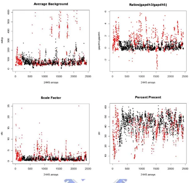
Initially, we have 1279 arrays that pass our quality control criteria. We will use these 1279 arrays to build up our reference set. Further details of delete step contained in Table 3.1, and Figure 3.1 show a general overview about the distributions of those delete arrays over all 2445 arrays in four values: “avbg”, “sfs”, “pp” and “ratios”.

3.2 To preprocess our reference set and classify arrays by tissues

First, we use justRMA to preprocessing our 1279 arrays in R-2.3.0. We classify these 1279 arrays in the reference set by their tissue types. Seventy-four tissue types were

obtained. There are 8 tissue types that only contain one array and 4 tissue types that contain more than 50 arrays. The biggest tissue type is “whole blood” with 67 arrays in there. The distribution of the number of arrays in each tissue type is in Table 3.2. Table 3.3 shows those 74 tissue types and the number of arrays they contain. Then we randomly choose 74 arrays by tissue type (a tissue type pick one array as the representation of that tissue type). We use these 74 arrays as the representation of all 1279 arrays in our reference set to build up a set of parameters from the function “rma.para” in package “RefPlus” (Harbron C. et

al. 2007). Then we obtain two sets of parameters: “Reference.Quantiles” and

“probe.effects”, and later we can use an R function “rmaplus” with these two sets of parameters to preprocess new target arrays without re-preprocessing them along with the reference set together again.

3.3 To find out our training dataset and preprocess it by RefPlus parameters

We found a dataset that had both control and case samples and did not overlap with our arrays in the reference set. The dataset is from the Karolinska Hospital 1994-1996 that publish on web of GEO (Pawitan et al. 2005). There are 38 arrays as poor prognosis and 121 arrays as good prognosis, where poor prognosis was defined as distant relapse or death year less than 5 by any cause. Arrays from poor prognosis are treated as case samples (disease) and arrays from good prognosis are treated as control samples (non-disease). These “training” arrays with known disease statuses are preprocessed, using R function

rmaplus and parameters “Reference.Quantiles” and “probe.effects” from our reference

training set.

3.4 Six classification rules

Due to the computer capacity, we choose 38 arrays from poor prognosis and 70 arrays from good prognosis to be our training set (totally containing 108 arrays). Let’s define

:

D diseased and ND non diseased: − ,

= ij

d the expression value of the jth probe in the ith “diseased” array,

= ij

nd the expression value of the jth probe in the ith “non-diseased” array,

= ij

ref the expression value of the jth probe in the ith “reference” array,

∑

= the mean expression value of the jth probe over all n₁ diseased arrays,

∑

= the mean expression value of the jth probe over all n₂ non-diseased arrays,

∑

= the mean expression value of the jth probe over all n reference arrays, ₃

= j

X the expression value of the jth probe in the “newly” observed array X ,

= ) ( j d X

D the “distance” between new observation X and the disease group

in the jth probe, =

) ( _j nd X

D the “distance” between new observation X and the non-disease group

in the jth probe, ) ( ) ( ) (Xj Dnd Xj Dd Xj Diff = − , where j=1,…,22283.

In the following, we will establish various ways for calculating the “distance”, and then develop their corresponding classification rules.

3.4.1 Method 1 (corrected by the reference set and training groups)

Due to the apparent “probe effect”, the distance between new observation X and the disease group in the jth probe is corrected with the distance between the disease group and

the reference group in the jth probe. The same correction is also applied to the distance with the non-diseased group. Therefore, we define

| | | | ) ( j j _.j _.j _.j d X X d d ref D = − − − , | | | | ) ( j j _.j _.j _.j nd X X nd nd ref D = − − − , 22283 , , 1 ), ( ) ( ) (X =D X −D X j= _L Diff _{j nd j d j} .

If most of the probes withDiff(Xj)≤0, we assign new observation X to ND (the non-diseased group).

If most of the probes withDiff(X_j)>0, we assign new observation X to D (the diseased group).

We proposed to do the following hypothesis testing: 0:

H new observation X belongs to ND (the non-diseased group)

vs. H₁:new observation X belongs to D (the diseased group)

Test statistic = ~ ( 1) )) ( ( )) ( ( 0 − = t p p X Diff SD X Diff E T H ,

where ))E(Diff(X is the sample mean of Diff(X₁),_L,Diff(X_p), ))SD(Diff(X is the

sample standard deviation of Diff(X₁),_L,Diff(X_p) , and p=22283. If reject null hypothesis, we assign new observation X to disease group. If accept null hypothesis, we assign new observation X to non-disease group. To calculate the classification error of the proposed rule, we perform the leave-one-out cross validation on the training set. In other words, (1) omit one observation from the training set and develop classification Method 1 based on the remaining observations, (2) classify the “holdout” observation, using the rule constructed in (1), and (3) repeat steps (1) and (2) for all observations in the training set. As a result, 74 out of all 108 arrays in the training set were classified correctly by Method 1.

Here, the distance is corrected with the distance between new observation and the reference group. | | | | ) ( j j _.j j _.j d X X d X ref D = − − − , | | | | ) ( j j _.j j _.j nd X X nd X ref D = − − − , 22283 , , 1 ), ( ) ( ) (X =D X −D X j= _L Diff _{j nd j d j} .

We then perform the same hypothesis test as what Method 1 does. As the result of the leave-one-out cross validation, 80 out of all 108 arrays in the training set were classified correctly by Method 2.

3.4.3 Method 3 (no corrected)

Here, no correction for the distance is done. | | ) ( _{j j . j} d X X d D = − , | | ) ( _{j j . j} nd X X nd D = − , 22283 , , 1 ), ( ) ( ) (X =D X −D X j= _L Diff _{j nd j d j} .

We then perform the same hypothesis test as what Method 1 does. As the result of the leave-one-out cross validation, 80 out of all 108 arrays in the training set were classified correctly by Method 3.

3.4.4 Method 4 (corrected by multiplying the standard deviation of the jth probe in

the reference set)

Assuming that the probes with large standard deviations in the reference set tend to be more capable of discriminating between diseased and no-diseased groups than the probes with small standard deviations, we use the standard deviation of each probe in the reference set as the weight when calculating the distance. Therefore, let

) ( | | ) ( j j _.j _.j d X X d SD ref D = − × ,

) ( | | ) ( j j _.j _.j nd X X nd SD ref D = − × , 22283 , , 1 ), ( ) ( ) (X =D X −D X j= _L Diff _{j nd j d j} ,

whereSD(ref_{. j}) is the sample standard deviation of ref _j ref_{n j}

3

, ,

1 L .

We then perform the same hypothesis test as what Method 1 does. As the result of the leave-one-out cross validation, 80 out of all 108 arrays in the training set were classified correctly by Method 4.

3.4.5 Method 5 (corrected by multiplying the standard deviation of the jth probe in

the reference set and dividing the standard deviation of the jth probe in the

training group)

In addition to the assumption in Method 4, we also consider the different effects in the diseased and the non-diseased groups. We propose to correct the distance with the diseased group by dividing the standard deviation of each probe in the diseased group and the distance with the non-diseased group by dividing the standard deviation of each probe in the non-diseased group. Therefore,

) ( ) ( | | ) ( . . . j j j j j d d SD ref SD d X X D = − × , ) ( ) ( | | ) ( . . . j j j j j nd nd SD ref SD nd X X D = − × , 22283 , , 1 ), ( ) ( ) (X =D X −D X j= _L Diff _{j nd j d j} ,

whereSD(d_{. j}) is the sample standard deviation of d _j d_nj

1

, ,

1 L , and SD(nd. j) is the sample standard deviation of nd _j nd_{n j}

2

, ,

1 L .

We then perform the same hypothesis test as what Method 1 does. As the result of the leave-one-out cross validation, 70 out of all 108 arrays in the training set were classified correctly by Method 5.

3.4.6 Method 6 (corrected by dividing the standard deviation of the jth probe in the

reference set)

Contrary to the assumption in Method 4, one might think that the probes with large standard deviations in the reference set tend to be more “unstable” and thus can reduce their ability in discriminating between diseased and no-diseased groups. We thus use the inverse of the standard deviation of each probe in the reference set as the weight when calculating the distance. Therefore, let

) ( 1 | | ) ( . . j j j j d ref SD d X X D = − × , ) ( 1 | | ) ( . . j j j j nd ref SD nd X X D = − × , 22283 , , 1 ), ( ) ( ) (X =D X −D X j= _L Diff _{j nd j d j} .

We then perform the same hypothesis test as what Method 1 does. As the result of the leave-one-out cross validation, 80 out of all 108 arrays in the training set were classified correctly by Method 6.

3.5 To obtain the list of genes with multiple modes from the idea of bar code

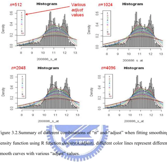
All 1279 reference files were preprocessed using justRMA of R, and then we obtain the empirical expression distribution across tissues for each gene. The empirical distribution is obtained by fitting a density smoother for each gene, using R function density n adjust , ( , ) where n is the number of equally spaced points at which the density is to be estimated

and adjust is the bandwidth used. We try some different combinations of n and adjust

to fit the density distribution function and show the fit result in the following graph (Figure 3.2). Then we decide to use n=512,adjust = for all genes to fit their empirical density 3 functions. After the density function of each gene is fitted, we check the changes of slopes of these functions to define whether or not the gene has multiple modes. If the slope transfers from positive to negative, this means there is a mode in this density distribution. If

transferring the slope from positive to negative more than once, then we define this gene to have a “multiple-mode” density distribution. Overall, we find 5005 multiple-mode genes from all 22283 genes in the HG-U133A GeneChip, based on our 1279 reference set arrays. These 5005 genes are used for creating our classification rule.

3.6 Do classification procedure again (Method 1~Method 6) with multiple-mode

genes

Here we perform classification Method 1~Method 6 described in sections 3.4.1-3.4.6 by using only 5005 genes with multiple modes. The new results are compared with the ones based on all 22283 genes.

3.7 Classify testing set by PAM

For the purpose of comparison, the training set is cross-validated by PAM (Tibshirani et

al., 2002). We use the functions in R package “pamr”. The “pamr.train” is a function to

train a nearest shrunken centroid classifier. The “pamr.predict” is a function for producing predicted information from a nearest shrunken centroid fit. “pamr.predict” also gives a cross-tabulation of true versus predicted classes for the fit returned by “pamr.cv” or “pamr.train” at the specified threshold. Here, we use “pamr.train” and threshold=1. When classifying by PAM, we also run twice: one using all 22283 genes and the other using only 5005 multiple-mode genes.

4. Result

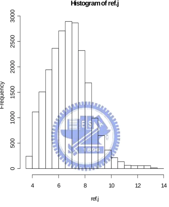
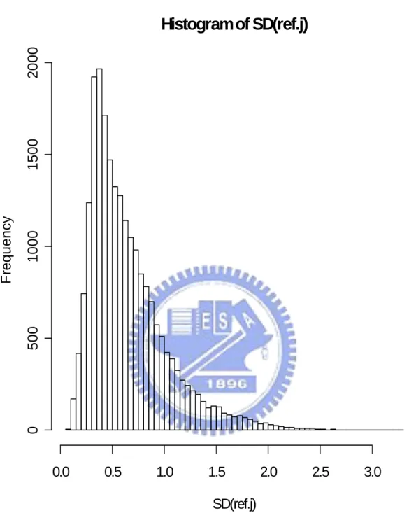
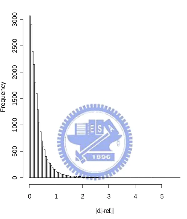
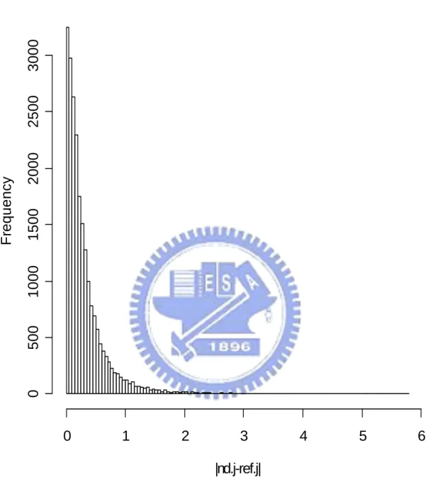
In the end, we do all six proposed methods and PAM twice: one using all 22283 genes and the other using only 5005 multiple-mode genes. Figure 4.1 show the histogram of the mean expression value of each gene in reference set. We find that the distribution of mean expression value follow a non-symmetrical and one-mode distribution. So we assume that mean expression value of each gene present the probe effect of each gene in Microarray HGU133A chip. And we use those mean expression values to modify the definition of our distance between observation array and different groups (using in Method 1 and Method 2). Figure 4.2 show the histogram of the sample standard deviation of expression value for each gene in reference set. We find that most sample standard deviations of expression value for each gene in reference set are near to 0.5 and the distribution of the sample standard deviation of expression value for each gene is non-symmetrical. So we think each gene have different contributions to classification. And we decide to use the sample standard deviation of each gene in reference set to be the weight of each gene in classification and present the different contribution of each gene in classification (using in Method 4, Method 5 and Method 6). Figure 4.3 and Figure 4.4 show the histograms of the absolute different value of mean expression for each gene between disease group, non-disease group, and reference set separately. Figure 4.3 and Figure 4.4 both show us that there are different “distances” of each gene from group to reference set. That support our decision to build up classifier 1 (Method 1). The results of the leave-one-out cross validation are shown in Table 4.1. We can find that classify with all 22283 genes and with 5005 multiple-mode genes get similar result (there is no big different in classify correctly rate). We also can think it means 5005 multiple-mode genes can represent all 22283 genes and the information that contained by all 22283 genes. We can use these 5005 multiple-mode genes to build up our classifier without choosing special genes by tissues types or diseases and can saving our computer capacity and time from replace 22283 genes

by 5005 multiple-mode genes. And although the result of PAM is better than the result of our six classifiers, it still exist about seventy percent successive-classified rate of our classifiers. It shows us that simple T-test still performs a not-bad result in classification. Figure 4.1 show the detail of all result, where a point means we classify successfully once and green points and black points were the results from doing simple t-test by 5005 multiple-mode genes and by all 22283 genes respectively. There are some arrays that always been classified to wrong class no matter what classifier we used (PAM or M1~M6).

5. Conclusion and discussion

Due to our study result we demonstrate that expressed genes are those genes with multiple-mode in distribution and simple t test also can be applicable in classification or build a classifier. Using simple t test to build up a classifier is easier than other classifiers and do not need to fit some complicated data selection rules. In future, we think that we can continue to investigate that why some arrays always been classified incorrectly by all classifier even by PAM. For example we can try to provide criteria for well separated genes and not well separated genes among 5005 2-or-more-mode genes and the difference between two kinds of genes show in Figure 5.1.

References

ACBB(applied computational biology and bioinformatics). Simpleaffy:easy analysis routines for Affymetrix data

http://bioinformatics.picr.man.ac.uk/research/software/simpleaffy/index.html

ACBB(applied computational biology and bioinformatics). Using Simpleaffy for Affymetrix QC

http://bioinformatics.picr.man.ac.uk/research/software/simpleaffy/qcstats.html

Affymetrix GeneChip 中文快速攻略本

http://ipmb.sinica.edu.tw/affy/document/user_guide_c.pdf

Bolstad B. (2008). Some FAQ about computing the RMA expression measure http://bmbolstad.com/misc/ComputeRMAFAQ/ComputeRMAFAQ.html

Bittner M, et al. (2000). “Molecular classification of cutaneous malignant melanoma by gene expression profiling.” Nature 406, 536-540.

Bolstad BM, Irizarry RA, Astrand M, and Speed TP. (2003). “A Comparison of Normalization Methods for High Density Oligonucleotide Array Data”. Bioinformatics 19(2):185-193

Gentleman R, Carey VJ, Huber W, Irizarry RA, Dudoit S. (2005). “Bioinformatics and Computational Biology Solutions Using R and Bioconductor.” Springer. Chapters 12, 13 and 24

Harbron C, Chang KM, and South MC. (2007). “RefPlus: an R package extending the RMA Algorithm”. Vol. 23 no. 18 2007, pages 2493-2494, doi: 10.1093/bioinformatics/btm357.

Irizarry RA, Bolstad BM, Collin F, Cope LM, Hobbs B and Speed TP. (2003). “Summaries of Affymetrix GeneChip probe level data”. Nucleic Acids Research 31(4):e15

Irizarry RA, Hobbs B, Collin F, et al. (2003). “Exploration, Normalization, and Summaries of High Density Oligonucleotide Array Probe Level Data.” Biostatistics .Vol. 4, Number 2: 249-264

Ivliev AE. (2008). “Microarray retriever: a web-based tool for searching and large scale retrieval of public microarray data.” Nucleic Acids Research, 2008

Katz S, Irizarry RA, Lin X, Tripputi M and Porter MW. (2006). “A summarization approach for Affymetrix GeneChip data using a reference traing set from a large, biologically diverse database”. BMC Bioinformatics 2006, 7:464

PAM: Prediction Analysis for Microarrays. Class Prediction and Survival Analysis for Genomic Expression Data Mining.

http://www-stat.stanford.edu/~tibs/PAM/

Prediction Analysis for Microarrays, for the R package. http://www-stat.stanford.edu/%7Etibs/PAM/Rdist/index.html

Pawitan Y, et al. (2005). “Gene expression profiling spares early breast cancer patients from adjuvant therapy: derived and validated in two population-based cohorts.” Breast Cancer Research 2005

Tibshirani R, Hastie T, Narashiman B and Chu G. (2002). "Diagnosis of multiple cancer types by shrunken centroids of gene expression". PNAS 2002 99:6567-6572 (May 14).

Wilson C, Pepper SD, Miller CJ. (2009). “QC and Affymetrix data” http://bioinformatics.picr.man.ac.uk/downloads/QCandSimpleaffy.pdf

Zilliox MJ and Irizarry RA. (2007). “A gene expression bar code for microarray data”. Nature Methods, 2007

Figure 2.1. The design of probes for Microarray HGU133A chip

Figure 3.1.The distributions of those delete arrays over all 2445 arrays in four quality assessment metrics. The red dots represent all deleted data. The block dots are the data still kept after all the quality assessment steps.

Figure 3.2.Summary of different combinations of “n” and “adjust” when fitting smoothing density function using R function density(n,adjust), different color lines represent different smooth curves with various “adjust” values.

Histogram of ref.j

ref.j

F

requenc

y

4

6

8

10

12

14

0

5

00

1000

1500

2000

2500

3000

Histogram of SD(ref.j)

SD(ref.j)

F

requenc

y

0.0

0.5

1.0

1.5

2.0

2.5

3.0

0

500

1000

1

500

2

000

Figure 4.2. The histogram of the sample standard deviation of expression value for all genes in reference set.

Histogram of |d.j-ref.j|

|d.j-ref.j|

F

requenc

y

0

1

2

3

4

5

0

5

00

1000

1500

2000

2500

3000

Figure 4.3. The histogram of absolute different value of mean expression between disease group in testing set and reference set.

Histogram of |nd.j-ref.j|

|nd.j-ref.j|

F

requenc

y

0

1

2

3

4

5

6

0

500

1000

1500

2000

2500

3000

Figure 4.4. The histogram of absolute different value of mean expression between non-disease group in testing set and reference set.

Figure 4.5. Summary of classification results, where a point means we classify successfully once and green points and black points were the results from doing simple t-test by 5005 multiple-mode genes and by all 22283 genes respectively.

Table 3.1.Summary of QC step GEO AE Total Before QC 1886 559 2445 Scale factor -359 -112 -471 Averages background -56 0 -56 3＇/5＇ ratios -302 -98 -400

Percent present calls -4 -13 -17

After QC 1165 336 1501

Remove same type 943 336 1279

Table 3.2.The distribution of the number of arrays in each tissue type number of arrays in one

tissue type

1 2~5 6~10 11~20 21~30 31~50 51~70 total

Table 3.3.The number of arrays in each tissue type

Tissue n Tissue n Tissue n Tissue n

beta cell islets 1 Theca cell 4 umbilical cord blood 13 brain 29

medulla oblongata 1 Normal_Ovary 5 thymus 14

unknow tissue type 29 Normal Breast 1 thyroid gland (thyrocytes) 7 Post-mortem medial

substantia nigra 15 skeletal muscle 33 Normal Colon 1 Normal Spleen 7 skin 16 Normal Caudate Nucleus 33 Normal Corpus

1 adipose tissue 8 Undifferentiated human ES cells 16 prefrontal cortex 33 Normal Stomach 1 Normal cervix 8 lymphoblastoid cell

lines 17 duodenal tissue 40 Normal Thalamus

1 prostate 8 Human optic nerve head astrocytes 18 human post-mortem brain tissue 43 normal tissue adjacent to Renal Cell Carcinoma 1 TERV (cell line) 8 hypothalamus 22 peripheral blood (human PBMC) 47 Normal Adrenal

Gland 2 smooth muscle 9 liver 22

white blood cells 48 Fetal Cartilage from Distal Femur 2 primary fibroblast cell line

Normal Heart

2

PBSC CD34

selected cells 10 T cells resting 23

Human umbilical vein endothelial cells 53 Pancreas 2 Baseline

macrophages 11 cerebellum 24 bone marrow 56 spinal cord 2 Normal Bladder 11 Normal Kidney 25 lung 63 salivary gland 2 testis 11 uterus 25 whole blood 67

Pituitary 2 tonsil 11 esophageal epithelium 26 Normal Amygdala

3 synovial

membrane 11 Frontal Cortex 26

intestinal

xenograft tissue 3 B-cells 12

blood (cell type : mononuclear cells from venous blood)

26 Trachea 3 SH-SY5Y neuroblastoma cells 12 blood (monocyte) 27 Pulp tissue 4 Stratagene Universal Human Reference RNA

12 placental basal plate 27

occipital lobe 4

peripheral blood

Table 4.1The results of the leave-one-out cross validation, using various classification rules The number of corrected classified arrays Metho d 1 Metho d 2 Metho d 3 Metho d 4 Metho d 5 Metho d 6 Metho d 7 (PAM) Total

Use all probes 74 80 80 80 70 80 88 108

(%) 68.52 74.07 74.07 74.07 64.82 74.07 81.84 100 Use 5005

probes

70 77 77 79 69 78 87 108