偏常態因子信用組合下之效率估計值模擬 - 政大學術集成

全文

(1)國立政治大學統計學系博士學位論文. 指導教授：劉惠美博士. 偏常態因子信用組合下之效率估計值模擬政治. 大. 立. ‧. ‧ 國. 學. Efficient Simulation in Credit Portfolio. y. Nat. n. al. er. io. sit. with Skew Normal Factor. Ch. engchi. i Un. v. 研究生：林永忠撰中華民國一百零一年七月.

(2) 中文摘要. 在因子模型下，損失分配函數的估算取決於混合型聯合違約分配。蒙地卡羅是一個經常使用的計算工具。然而，一般蒙地卡羅模擬是一個不具有效率的方法，特別是在稀有事件與複雜的債務違約模型的情形下，因此，找尋可以增進效率的方法變成了一件迫切的事。. 對於這樣的問題，重點採樣法似乎是一個可以採用且吸引人的方法。透過改. 治政模型。因此，我們將應用重點採樣法來估計偏常態關聯結構模型的尾部機率。這大立篇論文包含兩個部分。Ⅰ：應用指數扭轉法---一個經常使用且為較佳的終點採樣變抽樣的機率測度，重點採樣法使估計量變得更有效率，尤其是針對相對複雜的. ‧ 國. 學. 技巧---於條件機率。然而，這樣的程序無法確保所得的估計量有足夠的變異縮減。此結果指出，對於因子在選擇重點採樣上，我們需要更進一步的考慮。Ⅱ：進一. ‧. 步應用重點採樣法於因子；在這樣的問題上，已經有相當多的方法在文獻中被提. sit. y. Nat. 出。在這些文獻中，重點採樣的方法可大略區分成兩種策略。第一種策略主要在. io. er. 選擇一個最好的位移。最佳的位移值可透過操作不同的估計法來求得，這樣的策略出現在 Glasserman 等(1999)或 Glasserman 與 Li (2005)。. n. al. Ch. engchi. i Un. v. 第二種策略則如同在 Capriotti (2008)中的一樣，則是考慮擁有許多參數的因子密度函數作為重點採樣的候選分配。透過解出非線性優化問題，就可確立一個未受限於位移的重點採樣分配。不過，這樣的方法在尋找最佳的參數當中，很容易引起另一個效率上的問題。為了要讓此法有效率，就必須在使用此法前，對參數的穩健估計上，投入更多的工作，這將造成問題更行複雜。. 本文中，我們說明了另一種簡單且具有彈性的策略。這裡，我們所提的演算法不受限在如同 Gaussian 模型下決定最佳位移的作法，也不受限於因子分配函數參數的估計。透過 Chiang, Yueh 與 Hsie (2007)文章中的主要概念，我們提供了重點採樣密度函數一個合理的推估並且找出了一個不同於使用隨機近似的演算法來 i.

(3) 加速模擬的進行。. 最後，我們提供了一些單因子的理論的證明。對於多因子模型，我們也因此有了一個較有效率的估計演算法。我們利用一些數值結果來凸顯此法在效率上，是遠優於蒙地卡羅模擬。. 關鍵字：蒙地卡羅模擬；重點採樣法；信用風險組合；變異縮減。. 立. 政治大. ‧. ‧ 國. 學. n. er. io. sit. y. Nat. al. Ch. engchi. ii. i Un. v.

(4) ABSTRACT. Under a factor model, computation of the loss density function relies on the estimates of some mixture of the joint default probability and joint survival probability. Monte Carlo simulation is among the most widely used computational tools in such estimation. Nevertheless, general Monte Carlo simulation is an ineffective simulation approach, in particular for rare event aspect and complex dependence between defaults of multiple obligors. So a method to increase efficiency of estimation is necessary.. 立. 政治大. Importance sampling (IS) seems to be an attractive method to address this problem.. ‧ 國. 學. Changing the measure of probabilities, IS makes an estimator to be efficient especially. ‧. for complicated model. Therefore, we consider IS for estimation of tail probability of. sit. y. Nat. skew normal copula model. This paper consists of two parts. First, we apply exponential. io. er. twist, a usual and better IS technique, to conditional probabilities and the factors. However, this procedure does not always guarantee enough variance reduction. Such. al. n. iv n C result indicates the further consideration h e ofn choosing g c h i ISUfactor density.. Faced with this problem, a variety of approaches has recently been proposed in the literature ( Capriotti 2008, Glasserman et al 1999, Glasserman and Li 2005). The better choices of IS density can be roughly classified into two kinds of strategies. The first strategy depends on choosing optimal shift. The optimal drift is decided by using different approximation methods. Such strategy is shown in Glasserman et al 1999, or Glasserman and Li 2005.. iii.

(5) The second strategy, as shown in Capriotti (2008), considers a family of factor probability densities which depend on a set of real parameters. By formulating in terms of a nonlinear optimization problem, IS density which is not limited the determination of drift is then determinate. The method that searches for the optimal parameters, however, incurs another efficiency problem. To keep the method efficient, particular care for robust parameters estimation needs to be taken in preliminary Monte Carlo simulation. This leads method to be more complicated.. 政治大 enough to be applied in Monte 立Carlo setting. Indeed, our algorithm is not limited to the In this paper, we describe an alternative strategy that is straightforward and flexible. ‧ 國. 學. determination of optimal drift in Gaussian copula model, nor estimation of parameters of factor density. To exploit the similar concept developed for basket default swap. ‧. valuation in Chiang, Yueh, and Hsie (2007), we provide a reasonable guess of the. Nat. sit. y. optimal sampling density and then establish a way different from stochastic. n. al. er. io. approximation to speed up simulation.. Ch. engchi. i Un. v. Finally, we provide theoretical support for single factor model and take this approach a step further to multifactor case. So we have a rough but fast approximation that execute entirely with Monte Carlo in general situation. We support our approach by some portfolio examples. Numerical results show that such algorithm is more efficient than general Monte Carlo simulation.. Keywords: Monte Carlo simulation; Importance Sampling; Portfolio credit risk; Variance reduction.. iv.

(6) CONTENTS. 中文摘要 ............................................................................................................................i ABSTRACT .................................................................................................................... iii CONTENTS ......................................................................................................................v LIST OF FIGURES ..........................................................................................................vi LIST OF TABLES .......................................................................................................... vii Chapter 1 Chapter 2. 治政大 Portfolio Credit Risk Models ..................................................................4 立. Introduction..............................................................................................1. The Portfolio Loss Distribution......................................................................4. 2.2. Skew Normal Distribution and Its Properties.................................................6. ‧ 國. Variance Reduction Methodology ..........................................................9. ‧. Chapter 3. 學. 2.1. IS Method .......................................................................................................9. 3.2. IS Conditional on SN Factor ........................................................................12. 3.3. IS For SN Factor...........................................................................................17. y. sit. er. io. al. iv n C The New Method forhSN ...........................................................39 i U e nFactor gch n. Chapter 4. Nat. 3.1. 4.1. Extension of CYH Importance Sampling Algorithm ...................................39. 4.2. The Proposed algorithm for Skew Factor Model .........................................46. 4.3. Asymptotic Optimality .................................................................................51. Chapter 5. Implementation Issues ...........................................................................55. Chapter 6. Concluding Remarks .............................................................................59. REFERENCE ..................................................................................................................61. v.

(7) LIST OF FIGURES. Fig. 2-1. The density function of SN (0,1, λ ) ..................................................................8. Fig. 3-1 A specific example with ρ = 0.3 , b = 0.2 , m = 100 ,.........................................16 Fig. 3-2 Comparisom of − Fm ( z ) / m under different loading values ............................17 Fig. 3-3 Graph of Fm (t ) + Fm' (t )( z − t ) for a single factor ..........................................21 Fig. 3-4 Comparison of rate function under λ < 0 ....................................................36. 立. 政治大. ‧. ‧ 國. 學. n. er. io. sit. y. Nat. al. Ch. engchi. vi. i Un. v.

(8) LIST OF TABLES. Table 4-1：Comparison of different methods for m = 250 ;ν = 12 ; q = 0.25 ...................43 Table 4-2：Comparison for (m, m1 ; a1 ; a2 ; p1 ; p2 ) = (1, 000;150;0.8;0.7;0.05;0.001) ..................45 Table 5-1: Variance Reduction for decreasing λ . ..........................................................56 Table 5-2: Variance Reduction for increasing b . ...........................................................56 Table 5-3: Variance Reduction for increasing ρ . ...........................................................57. 政治大. Table 5-4: Variance Reduction for increasing q . ...........................................................58. 立. ‧. ‧ 國. 學. n. er. io. sit. y. Nat. al. Ch. engchi. vii. i Un. v.

(9) Chapter 1. Introduction. The impressive development of the securities markets has led financial institutions to quantify their risk by stochastic models. A main component of financial risk is credit risk, in particular for rare event aspect and complex dependence between defaults of multiple obligors. By referring to losses resulting from the default of obligor, the bank and other institutions therefore make a contractual payment for structural financial products.. 政治大. An important feature of modern credit risk management is to capture the effect of. 立. dependence among obligors. In the development of commercial models, the dependence. ‧ 國. 學. structure among obligors is specified through a set of “systematic factors”. It is. ‧. so-called factor copula model approach, which is originally associated with J. P.. sit. y. Nat. Morgan’s CreditMetrics system. To match the observed financial data, the methodology. io. er. to find an adequate factor copula to model dependencies becomes very popular. There are a lot of papers to address better empirical fits of observed data by copula factor. al. n. iv n C models. Examples are the normal copula U Finger& Bhatia (1997), the h e nmodel g c hini Gupta, Student-t copula in Schloegl and O’Kane (2005), the double t distribution copula in Hull and White (2004) and Marshall-Olkin copula in Andersen and Sidenius (2005).. In practice, normal and Student-t copula models are two of the most widely used models. It has been incorporated into many popular risk management systems. However, more empirical works have argued the leptokurtic and asymmetric factor distribution rather than symmetric distribution. In fact, the feature of leptokurtic and asymmetry leads to significant inaccuracies in assessing the probability of extreme cases like large 1.

(10) portfolio losses and default threshold of obligor. This result shows the importance of choosing an appropriate factor distribution for application of copula model.. In our opinion, the skew normal (SN) distribution can come up with the leptokurtic and asymmetric features. However, like most approximations in different copula cases (Glasserman (2004); Kostadinov (2005)), there are no closed form analytical results which provide the error bound of estimation. So we need a viable alternative which not only assess the performance of default but provide more information of error.. 政治大 Monte Carlo simulation立 is the most widely used in the estimation of default. It has. ‧ 國. 學. the advantage of being very general and disadvantage of being slowly. For estimating rare event default probability, the generalization of this method can serve the. ‧. complicated copula well, but disadvantage cause time-consuming problem. This. Nat. sit. n. al. er. io. efficiency.. y. motivates research on variance reduction methods like IS to increase simulation. Ch. engchi. i Un. v. For normal copula, a special case of skew normal factor model, Glasserman and Li (2005) (henceforth GL) propose a process by applying two step IS. Such approach speed up the occurrence of default event to achieve optimality of simulation. However, portfolio with SN factor is unlike the normal case, the asymmetry of SN distribution leads the procedure developed in GL is not applicable here. Surprisingly, the application of exponential twisted shift, which is a usual and better IS technique, does not always guarantee efficient variance reduction. Hence, we need to search a new way to devise IS algorithm.. 2.

(11) Different from only considering adjustment of parameters, our approach emphasize on choosing “form” of IS density distribution. Our procedure consists of two parts. For the first step, we exploit independence property to apply IS technique to conditional probability. By this, we can reduce the part of total variance. For the second step, we eliminate the linear part of variability resulting from first step and simultaneously minimize residual volatility. Combine the two step, we then have an efficient algorithm.. The rest of this article is organized as follows. In the next chapter, In addition to. 政治大 also present the brief properties 立 of skew normal distribution. In Chapter 3, we review. the introduction of the credit risk copula model and importance sampling method, we. ‧ 國. 學. two-step IS method in GL and modify the procedure of applying exponential twist technique to factor. The modified procedure does not remain well behaved in different. ‧. shape parameter setting. Next, we extend a CYH procedure and build an efficient. Nat. n. al. Ch. engchi. 3. er. io. concluding remarks are presented in Chapter 6.. sit. y. algorithm in Chapter 4. Numerical examples are illustrated in Chapter 5 and finally the. i Un. v.

(12) Chapter 2. Portfolio Credit Risk Models. Credit portfolio models can be divided into reduced-form models and structural models. Discussions of several models have been put in the literatures of Crouhy et al.(2000), Bluhm et al.(2002) and McNeil et al.(2005). Different credit risk models differ in the mechanisms they use to capture dependence among obligors. In this paper, we consider the model approach similar to CreditMetricsTM (as in Gupta et al (1997) and Li (2000)), which is based on foundational work of Merton(1974). The default setting is incurred when the obligor’s shortage exceeds a default threshold.. 立. The Portfolio Loss Distribution. ‧ 國. 學. 2.1. 政治大. Consider a portfolio with m obligors, for the i th obligor, c i and X i denote the. ‧. exposure and status respectively. The exposure c i may be assumed to be stochastic.. y. Nat. er. io. sit. For sake of simplicity, we will assume c i to be deterministic and refer the reader to Glasserman, Kang, Shahabuddin (2008) for stochastic case. The i th obligor default if. n. al. X i exceed the threshold. i n U x , thenCthe portfolio loss L is hengchi i. v. m. m. Lm = ∑ ci I { X i > xi }. (2.1). i =1. In practice, threshold xi of i th obligor is chosen according to the marginal default probability pi so that P ( X i > xi ) = pi . This value pi is usually set based on the average historical default frequency with similar credit profiles. In the credit risk context, X i is usually given a financial interpretation. By such framework, Lm 4.

(13) models the loss of a portfolio of m obligors.. Our interest is in measuring the tail behavior of Lm , particularly for rare event. Since it is impossible to exactly compute the probability of large portfolio losses, we consider asymptotic regime which supports an analysis. Such regime is relevant to portfolios of high rated obligor, or measuring risk over a short period. We assume the default threshold for the individual obligor is xi = bi m , where marginal default of. 政治大. each obligor decrease when the number of obligors m increase. Our goal is to estimate. 立. the probability of {Lm > mq} , particular at large value of m and q .. ‧ 國. 學 j ≠ k . In general, the dependence. y. Nat. correlation structure between X j and X k ,. ‧. In the framework of copula, the dependence between defaults is determined by the. er. io. sit. structure is specified through a factor form. For example, if we set X k = ρ f + ε k for. n. ρ ∈ℜ where f and ε k a are normal random variable, we v obtain the dependence structure introduced in. i l C n TM U h e n. Ing caddition, CreditMetrics h i let X. k. = ε k /( ρ f ) with ρ > 0. and f and ε k follow Gamma and exponential distributions respectively, we get a way of introducing alternative dependence structure shown in Credit Suisse.. Here, we consider the dependence structure whose correlation is determined through a linear form, that is. d. d. j =1. j =1. X i = ∑ aij Z j + 1 − ∑ aij2 ε i. , i = 1, 5. ,m.

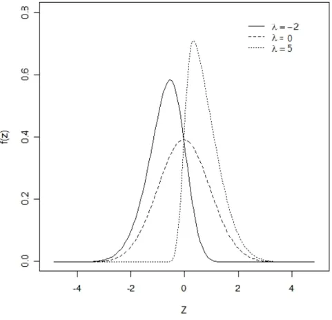
(14) where Z1 ,. , Z d and ε i are independent random variables. The systematic factor. , Z d affects multiple obligors simultaneously, but idiosyncratic factor ε i only. Z1 ,. influences the i th obligor. The coefficient aij is the loading for the j th factor and d. ∑a j =1. 2 ij. < 1 . Those loadings are assumed to be nonnegative. Although the condition is not. essential, the limitation can simplify our discussion, especially for large losses occur primarily because of highly positively correlated structure.. 政治大 In the following section, we will briefly introduce properties of distribution in SN 立. ‧ 國. ‧. 2.2. 學. copula model.. Skew Normal Distribution and Its Properties. Nat. io. sit. y. Let φ and Φ to be the standard normal probability density function and cumulative. n. al. er. density function respectively. The density function of a random variable Z j is given by. f ( z | μ;σ ; λ ) =. 2. σ. Ch φ(. engchi. z−μ. σ. )Φ (λ. z−μ. σ. i Un. v. ). , which is called SN distribution with location parameter μ ∈ℜ , scale parameter σ > 0 , and shape parameter λ ∈ℜ , denoted by Z ~ SN ( μ , σ 2 , λ ) . Let λ = 0 , we obtain the normal density. As λ → ∞ , it converges pointwise to half-normal density. The SN distribution was first introduced by O’Hagan and Leonard (1976) as a prior distribution for estimating a normal location parameter. It can be applied to different fields such as 6.

(15) economics, psychometry and so on. The moment generating function of SN ( μ , σ 2 , λ ) is given by. M (t | μ ; σ ; λ ) = 2 exp( μt +. (σ t ) 2 λ )Φ ( σ t) 2 1+ λ2. SN (0,1, λ ) is called the standard skew normal distribution. Some main properties of SN distribution are. 立. 政治大. if Z ~ SN (0,1, λ ) , then − Z ~ SN (0,1, −λ ) .. 2.. if Z ~ SN (0,1, λ ) , then Z 2 ~ χ12 .. 3.. E ( Z ) = μ + σ ( 2 / π )(λ / 1 + λ 2 ) .. 4.. Var ( Z ) = σ 2 {1 − (2 / π )λ 2 /(1 + λ 2 )} .. 5.. if Z1 ~ SN (0,1, λ ) and Z 2 ~ SN (0,1, 0) , then. ‧. ‧ 國. 學. 1.. n. er. io. ρ Z1 + 1 − ρ Z 2 2. sit. y. Nat. al. i n ρλ C U ~ SN (0,1, h e g c) h i 1 + λ (1n −ρ ) 2. v. 2. For more properties of the skew normal distribution, we refer the reader to Azzalini (1985); Gupta, Nguyen and Sanqui (2004); or Arnold and Lin(2004).. , d and ε i ~ SN (0,1, 0) , we can generate. Consider Z j ~ SN ( μ j , σ 2j , λ j ) , j = 1, Z j , j = 1,. , d and ε i in each replication for straightforward simulation. We compute. the value X i and determine whether the i th obligor default. From the default setting 7.

(16) of every obligor, we get the portfolio loss (2.1) and then evaluate the probability of {Lm > mq} . However, Monte Carlo estimator can’t achieve fixed relative precision when the value of threshold becomes large. This makes variance reduction methodologies potentially attractive. In the next chapter, we will introduce one method to make Monte Carlo effective.. 立. 政治大. ‧. ‧ 國. 學. n. er. io. sit. y. Nat. al. Fig. 2-1. Ch. engchi. i Un. v. The density function of SN (0,1, λ ). 8.

(17) Chapter 3. Variance Reduction Methodology. Although generally easy to be implemented, Monte Carlo simulations are infamous for being slow. Stochastic outcome is always affected by a statistical error which can generally be reduced to the expected accuracy by iterating the procedure for a long enough time. Usually, in order to reduce the error by a factor of ten one has to spend one hundred times as much computer time. This result contradicts practical necessity.. Several approaches to accelerate the efficiency of simulation, such as control. 政治大. variates, antithetic variables, and IS, have been proposed over the years. The goal of. 立. these technique is to reduce the variance of replications so that an expected level. ‧ 國. 學. accuracy can be obtained with a smaller number samples. Antithetic variables and. ‧. control variates are the most commonly used variance reduction techniques, but their. er. io. sit. y. Nat. effectiveness varies largely across applications, and is sometimes rather limited.. Different antithetic variables and control variates, IS generally involves a bigger. al. n. iv n C implementation effort and is less straightforward h e n g c h ito Uinclude in general Monte Carlo framework. Furthermore, when used improperly, such method will “increase” the variance of estimator. That is why it has not been employed much in professional. contexts until recently. For all that, its powerful variance reduction is potentially attractive.. 3.1. IS Method. IS method is a standard approach of variance reduction in Monte Carlo methods. The idea behind IS method is to reduce the statistical uncertainty of a Monte Carlo 9.

(18) calculation by focusing on the important region of space from which the random samples are drawn. For example, suppose we have to evaluate E f [G ( X )] where G (⋅). is a positive measurable function with respect to the probability space and f is the density function of X , we hence have another representation. E[G ( X )] = ∫ G ( x) f ( x)dx = ∫ G ( x). 立. f ( x) * f ( x)dx f * ( x). 政治大. 學. ‧ 國. where f * is another density function of X . The ratio is called likelihood ratio or Randon-Nikodym derivative. One can sample X from new density and obtain the f ( x) . Its variance, then, is shown to be f * ( x). ‧. unbiased estimator G ( x). n. Ch. engchi. er. io. al. sit. y. Nat. 2 ⎡ 2 ⎛ f (X ) ⎞ ⎤ 2 E ⎢G ( X ) ⎜ * ⎟ ⎥ − E [G ( X )] ⎢⎣ ⎝ f ( X ) ⎠ ⎥⎦. i Un. v. Indeed, we have the following optimal IS density function f opt to achieve zero variance . f opt ( x) =. 1 G ( x) f ( x) E[G ( X )]. Such a density exists, but it is not feasible to be found unless the desired quantity is known from the outset. Much of the literature on IS technique are focused on methods 10.

(19) of choosing a reasonable approximation of zero-variance IS density (Sadowsky and Bucklew (1990); Glasserman et al (1999); Capriotti (2008)). The effectiveness of IS mainly depend on how close between new density and zero-variance density is. Different methods of approximation to zero-variance density will lead to various computational performances. In view of practicability consideration, we turn our attention to the apparently weaker notations of effectiveness.. Consider an estimation of E[G ( X m )] where G ( X m ) is a function which. 政治大. decrease to zero as m → ∞ . Then an estimator G ( X m ). io. er. m→∞. y. ‧ 國. Nat. lim sup. ‧. f (Xm) ] f *(Xm ) <∞ E[G ( X m )]. Var[G ( X m ). 學. bounded relative error if it satisfies the requirement. sit. 立. f (Xm) is said to be of f *(Xm ). al. n. iv n C Additionally, an estimator is called h logarithm asymptotically e n g c h i U efficient or asymptotically optimal if it satisfies the requirement. 2 ⎡ ⎛ f ( X m ) ⎞⎟ ⎤⎥ 2 ⎢ ⎜ ⎟ ln E ⎢G ( X m ) ⎜ * ⎜⎝ f ( X ) ⎠⎟⎟ ⎥⎥ ⎢⎣ m ⎦ =2 lim m→∞ ln E[G ( X m )]. An estimator with bounded relative error can remain the number of replication bounded in a fixed bounded relative error. However, asymptotically optimal only ensure that the rate of decay of second moment achieves twice that of itself. By Jensen’s 11.

(20) inequality, this is the fastest possible rate of decrease for any unbiased estimator. By the simple algebra, we know that an estimator with bounded relative error is also asymptotically optimal. General Monte Carlo can’t achieve asymptotically optimal. For example, let. pm = P ( X > m) where X ~ N (0,1) , then a general Monte Carlo. estimator I { X > m} has the following result. ln E[ I 2 { X > m}] =1 m→∞ ln E[ I { X > m}] lim. IS Conditional立 on SN Factor. 學. ‧ 國. 3.2. 政治大. In this section, we apply the one-step of GL to the credit portfolio with skew normal. ‧. factors. To keep the notation simple, we restrict our attention to single factor. al. er. io. sit. y. Nat. homogeneous model, that is ci = d = 1 , ρi = ρ , bi = b and X i is given by. n. X i = ρ Z + 1− ρ 2 εi. Ch. engchi. i Un. v. Thus the total loss Lm can be written as. m. Lm = ∑ I {ρ Z + 1 − ρ 2 ε i > b m} i =1. Let Yi = I {ρ Z + 1− ρ 2 εi > b m} . Conditioning on Z = z , Yi is a Bermoulli. random variable and the conditional default probability p( z ) is given by. 12.

(21) p( z ) = P(Yi = 1| Z = z ) = Φ(. ρz −b m 1− ρ 2. ). The joint probability of (Y1 , , Ym ) is then given by. m. ∏ ( p( z )). Yi. (1− p ( z ))1−Yi. i =1. Consider a new probability q( z; θ ( z )) which is specified by. θ(z). (3.1). exp(ψ (θ ( z ); z )). 學 ‧. ‧ 國. pθ ( z ) ( z ) =. 立 p ( z )e. 政治大. where ψ (θ ( z ); z ) = ln(1 + p ( z )(eθ ( z ) −1)) . If we replace each probability p( z ) with a. y. Nat. er. io. sit. new probability pθ ( z ) ( z ) , then the estimation of E[ I {Lm > mq}] can be written as. al. n. iv n C ph(Z ) ⎤ ) e n) g( c1−hpi(ZU ) ⎥⎥ > mq}∏ (. ⎡ E ⎢⎢ I {Lm ⎢⎣. m. 1−Yi. Yi. i =1. 1− pθ ( Z ) ( Z ). pθ ( Z ) ( Z ). ⎥⎦. (3.1) is called exponential twist. If θ ( z ) > 0 , then pθ ( z ) ( z ) > p ( z ) ; the original probability correspond to θ ( z ) = 0 . The new measure can increase the default probability and so decrease the variance resulting from stochastic volatility.. Let ψLm (θ ( z ), z ) = ∑ i=1 ψ (θ ( z ); z ) , the corresponding likelihood ratio is simplified m. into 13.

(22) m. p( z ) Yi 1− p ( z ) 1−Yi −θ ( z ) Lm +ψLm ( θ ( z ), z ) ) ( ) =e 1− pθ ( z ) ( z ) θ ( z ) ( z). ∏( p i =1. , then we have an unbiased estimator. −θ ( z ) Lm +ψLm ( θ ( z ), z ). I {Lm > mq}e. (3.2). 政治大. for P ( Lm > mq ) . It remains to choose θ ( z ) to reduce the variance of (3.2). We know. 立. the fact that a key element of variance reduction is based on minimizing the second. ‧ 國. 學. moment. It is difficult to solve this problem directly, but minimizing the upper bound of the second moment is easy. For θ ( z ) , we know. n. Note that the function ψLm. sit. −2{θ ( z ) mq−ψLm ( θ ( z ), z )}. | Z = z] ≤ e. er. io. al. y. ‧. Nat. −2 θ ( z ) Lm + 2 ψLm ( θ ( z ), z ). E[ I {Lm > mq}e. iv n C U in z ),e z ) nisgstrictly (θ (h c h i convex. θ ( z ) and pass through. the origin. So the function θ ( z )mq − ψLm (θ ( z ), z ) is a concave function and the supremun is attained at just one point, which we denote by θm ( z; q ) . If p ( z ) ≥ q , then the maximum value occurs at θm ( z; q) = 0 ; otherwise, it occurs at the unique solution of. ∂ ψL (θm ( z; q), z ) = mq ∂θ ( z ) m. In this discussion, θm ( z; q) may be viewed as a measure of the conditional rarity of the 14.

(23) set {Lm > mq} . If {Lm > mq} is not rare event, we generate the Yi | Z = z from the original probability; otherwise we twist by θm ( z; q ) . Observe the set {Lm > mq} , any element of {Lm > mq} has the property. θm ( z; q) Lm ≥ θm ( z; q)mq ,. ,then we have the lower bound. −θm ( z; q) Lm + ψLm. 立. 治政 (θ ( z; q), z ) ≤ F ( z ) 大 m. m. ‧ 國. 學. Here Fm ( z ) = −θm ( z; q ) mq + ψLm (θm ( z; q), z ) ≤ 0 . This result shows that the asymptotic. ‧. of upper bound depend on the point q when we apply IS to conditional probability.. y. Nat. io. sit. This unique point q is called the dominating point. Essentially, the decreasing rate of. n. al. er. Fm ( z ) determines whether the new estimator achieve asymptotically optimal. Observe that the equation. E[ Lm | Z = z ] =. Ch. engchi. i Un. v. ∂ ψL (θm ( z; q), z ) ∂θ ( z ) m. = mq. holds. This fact indicates that the mean value of. Lm | Z = z will be shifted to the m. dominating point q if {Lm > mq} becomes rare event. More details about dominating point we refer the readers to Ney (1983) or Sadowsky and Bucklew (1990). 15.

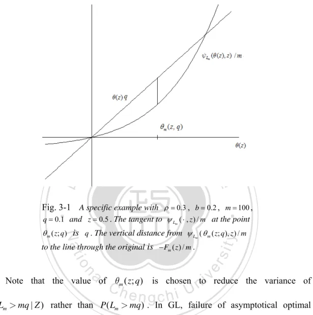
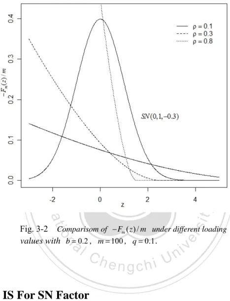
(24) 立. 政治大. ‧ 國. 學 ‧. Fig. 3-1 A specific example with ρ = 0.3 , b = 0.2 , m = 100 , q = 0.1 and z = 0.5 . The tangent to ψ Lm ( ⋅ , z ) / m at the point. y. Nat. θ m ( z; q ) is q . The vertical distance from ψ L ( θ m ( z; q ), z ) / m m. n. er. io. al. sit. to the line through the original is − Fm ( z ) / m .. i Un. v. Note that the value of θm ( z; q ) is chosen to reduce the variance of. Ch. engchi. P ( Lm > mq | Z ) rather than P ( Lm > mq ) . In GL, failure of asymptotical optimal results from the extra variability of Z . To analyze further, we should first realize how Fm ( z ) behave. Set loading ρ to be 0.1, 0.3, and 0.8 respectively, −Fm ( z ) / m is shown in Fig. 3-2.. In Fig. 3-2, it is obvious the larger value ρ is, the larger influence Z has. One step IS turns out to be less effective if the structure of Fm ( z ) has a width which depart from a constant. The behavior of Fm ( z ) indicates irrationality to neglect the effect 16.

(25) from the factor. Hence, we need to exploit proper IS method again to reduce the impact of factor.. 政治大. 立. ‧. ‧ 國. 學 sit. y. Nat. n. al. er. io. Fig. 3-2 Comparisom of − Fm ( z ) / m under different loading values with b = 0.2 , m = 100 , q = 0.1 .. 3.3. Ch. engchi. i Un. v. IS For SN Factor. As discussion in section 3.2, the key to improve efficiency of (3.2) is based on the elimination of residual randomness. Consider the (3.2) with θ ( z ) = θm ( z; q) , any estimator p mq has the variance decomposition as following. Var[ p mq ] = E[Var[ p mq | Z ]] + Var[ E[ p mq | Z ]]. 17.

(26) Applying IS to conditioning Z only makes E[Var[ p mq | Z ]] small. To get further improvement of efficiency, GL focus on the second term in the variance decomposition. By simple algebra, we know that the zero-variance IS density for Var[ E[ p mq | Z ]] is. 1 E[ I {Lm > mq}| Z = z ] f ( z | μ ; σ ; λ ) E[ I {Lm > mq}]. It is pity that sampling from this density is generally infeasible because of the. 政治大. normalization constant. For (μ, σ , λ ) = (0,1, 0) , GL thus suggest using original. 立. distribution with a appropriate mode as optimal density. Rather than choose IS density. ‧ 國. 學. arbitrarily, it is intuitively clear that shifting the mode makes the likelihood ratio inside. ‧. expectation to be small. For symmetric density, such strategy may make a substantial. y. Nat. variance reduction. Whenever zero variance density cannot be approximated only by. er. io. sit. shifting the mode, however, this algorithm becomes less beneficial. For instance, when the structure of E[ I {Lm > mq}| Z = z ] f ( z | μ ; σ ; λ ) has a width which is very different. al. n. iv n C from original density, shifting a drifthwill e nturng out c htoi beUineffective mechanism.. Faced with a similar problem, Capriotti (2008) uses Levenberg-Marquardt method to provide a reasonable IS density which is not limited the determination of drift. The implementation to determine the optimal parameters, however, incurs another efficiency problem. To keep the algorithm efficient, particular care for robust parameter estimation needs to be taken in preliminary Monte Carlo simulation. This leads algorithm to be more complicated.. 18.

(27) Instead of solving robust problem, we adopt another strategy to vanish randomness from Z . Let a new estimator applying IS for factor and conditional on factor to be. −2{θm ( Z ; q ) Lm −ψLm ( θm ( Z ; q ), Z )}. I {Lm > mq}e. W (Z ). (3.3). Here W ( Z ) = f ( z | μ ; σ ; λ ) / f * ( z | μ ;σ ; λ ) and f * ( z | μ ; σ ; λ ) denotes the IS density. We put emphasis on the variance of (3.3) rather than variance decomposition. Observe the second moment of (3.3). E ⎡⎢ I {Lm > mq}e ⎣. 立. 政治大 W 2 ( Z )⎤⎥ ⎦. 學. ≤ E ⎡⎢⎣ I {Lm > mq}e 2 Fm ( Z )W 2 ( Z )⎤⎥⎦. ‧. ‧ 國. −2 θm ( z ; q ) Lm + 2 ψLm ( θm ( z ; q ), z ). er. io. sit. y. Nat. ≤ ∫ e 2 Fm ( z )W 2 ( Z ) f * ( z | μ; σ; λ )dz. al. Directly minimizing second moment is difficult, a surrogate to guide proper IS. n. iv n C U bound of second moment. To density factor is required and thus we h econsider h iupper n g cthe. avoid integrating intricate function Fm ( z ) , we choose a different approximation. By the simple differentiation, we know Fm ( z ) is concave and then we have a loose upper bound by the first order Taylor expansion at point tm .. ∫. '. e 2 Fm ( z )W 2 ( Z ) f * ( z | μ; σ; λ )dz ≤ ∫ e 2{ Fm ( tm )+ Fm ( tm )( z−tm )}W 2 ( Z ) f * ( z | μ; σ; λ )dz '. = E[{e{ Fm (tm )+ Fm ( tm )( Z −tm )}W ( Z )}2 ]. 19.

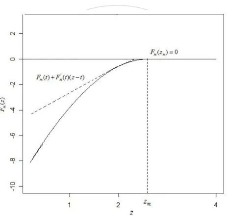
(28) Considering Jensen’s inequality, the inequality holds if. '. '. e Fm (tm )+ Fm (tm )( Z −tm )W ( Z ) = E[e Fm ( tm )+ Fm (tm )( Z −tm )W ( Z )] '. = E[e Fm (tm )+ Fm ( tm )( Z −tm ) ] ,. then the formulation yields. '. 政治大. e Fm (tm ) z f ( z | μ ;σ ; λ ) = f ( z | μ ;σ ; λ ) M Z ( Fm' (tm )) *. 立. (3.4). ‧ 國. 學. where M Z (⋅) denotes the moment generating function of Z . If we consider the. ‧. exponential twist density of Z as. n. Ch. engchi. er. io. al. sit. y. Nat. e tm z f ( z | μ;σ ; λ ) = f ( z | μ ;σ ; λ ) , M Z (tm ) *. i Un. (3.5). v. this connection of (3.4) and (3.5) implies that we can design a new exponential twisted IS density where tm = Fm' (tm ) , namely tm = arg max{Fm (t ) − t 2 / 2} t. Once we have selected the new IS density of Z , the algorithm proceeds as follows:. 20.

(29) 1.. Compute tm = arg max{Fm (t ) − t 2 / 2} t. 2.. Sample Z from f * ( z | μ ; σ ; λ ). 3.. Twisting the conditional default probability. 4.. Return the estimator pˆ ET = I {Lm > mq}e. 立. −θ m ( Z ; q ) Lm +ψ Lm (θ m ( Z ; q ), Z ) − tm Z + log M Z ( tm ). e. 政治大. ‧. ‧ 國. 學. n. er. io. sit. y. Nat. al. Ch. engchi. i Un. v. Fig. 3-3 Graph of Fm (t ) + Fm' (t )( z − t ) for a single factor with b = 0.2 , ρ = 0.3 , q = 0.1 and m = 1,000 .. By simple algebra, we know that the new IS distribution for Z is the closed skew normal CSN (tm ,1, λ , −λ tm ,1) if the original distribution is SN (0,1, λ ) . In fact, the appropriate IS distribution is not limited to the original distribution family and this result shows the difficulty in searching the optimal IS density. For more properties of closed skew normal one can see Graciela et al (2004). 21.

(30) Note that if λ = 0 , the choice of IS density coincides with the result of GL , that is a normal density with mean tm , namely CSN (tm ,1, 0, 0,1) .. Theorem 3.1 Consider a single factor homogeneous portfolio with the factor Z ~ SN (0,1, λ ) and. ε i ~ SN (0,1, 0) . Suppose the default and loss threshold are b m. and mq. respectively. Then the estimator pˆ ET satisfy. ‧ 國. 學. (a)For λ ≥ 0. 立. 政治大. 1 b2 lim log E[ I {Lm > mq}] = − 2 m →∞ m 2ρ. ‧. 1 b2 log E[( pˆ ET ) 2 ] = − 2 m →∞ m ρ. n. al. y. sit er. io. (b)For λ < 0. Nat. lim. i Un. 1 b2 lim log E{I {Lm > mq}} = − 2 (1 + λ 2 ) m →∞ m 2ρ. Ch. engchi. v. 1 b 2 1 + 2λ 2 log E{( pˆ ET ) 2 } = − 2 ( ) m →∞ m ρ 1+ λ 2 lim. Proof: The result would follow from a similar discussion in GL (2004). To start, we consider lower bound and upper bound of liminf and limsup respectively.. (a) λ ≥ 0 : First, we show that. 22.

(31) 1 b2 log E[ I {Lm > mq}] ≥ − 2 m 2ρ. lim inf m →∞. By conditional property, for any υ > 0 , we have the following result. E[ I {Lm > mq}] = E[ E[ I {Lm > mq} | p ( Z ) ≥ q + υ ]] = P ( Lm > mq | p ( Z ) ≥ q + υ ) P( p ( Z ) ≥ q + υ ) ≥ P ( Lm > mq | p ( Z ) = q + υ ) P( p ( Z ) > q + υ ). 立. 政治大. The inequality holds because Lm is binomially distributed with parameter m. ‧. ‧ 國. 學. and p ( Z ) .. Applying the lower bound (3.62) of Johnson et al. (1993), we have a lower bound for. y. Nat. n. al. er. io. the lower bound, we have. sit. the conditional probability P ( Lm > mq | p ( Z ) = q + υ ) ≥ 1/ 2 .Substituting the result into. E[ I {Lm > mq}] ≥. =. Ch. engchi. i Un. 1 P( p( Z ) > q + υ ) 2 b m + 1 − ρ 2 Φ −1 (q + υ ) 1 P( Z > ) 2 ρ. b m + 1 − ρ 2 Φ −1 ( q + υ ) 1 = {1 − FZ ( )} ρ 2. where FZ (⋅) denotes the cdf of Z and. 23. v.

(32) liminf m →∞. b m + 1 − ρ 2 Φ −1 ( q + υ ) 1 1 log E[ I {Lm > mq}] ≥ liminf log{1 − FZ ( )} m →∞ m m ρ. Applying l’Hospital’s rule, we obtain. liminf m →∞. b m + 1 − ρ 2 Φ −1 (q + υ ) 1 log{1 − FZ ( )} m ρ. b m − 1 − ρ 2 ξ1− q (1 + δ / ξ1− q ). 2. 立. b m − 1 − ρ 2 ξ1− q (1 + δ / ξ1− q ) 2 ρ mΦ (λ. b m − 1 − ρ ξ1− q (1 + δ / ξ1− q ). +. 2. 2ρ 2. ). 2mΦ (λ. ρ. b m − 1 − ρ 2 ξ1− q (1 + δ / ξ1− q ) 2ρ 2. } ). ‧. b2 2ρ 2. 政治) 大 2ρ. y. m →∞. m Φ (λ. io. sit. ρ. lim inf{. 2 m b m − 1 − ρ ξ1− q (1 + δ / ξ1− q ) 2. n. al. er. b. m →∞. Nat. =−. ρ. 2ρ. lim inf. ρ. 學. =−. b. ‧ 國. =−. +. which proves the formulation.. Ch. engchi. i Un. v. Next we show that. lim sup m →∞. 1 a2 log E{( pˆ ET ) 2 } ≤ − 2 ρ m. Write E{( pˆ ET ) 2 } as. E{( pˆ ET ) 2 } = E{I {Lm > mq}exp{−2θ m ( Z ; q) Lm + 2ψ Lm (θ m ( Z ; q ), Z ) − 2tm Z + 2 ln M Z (tm )}} 24.

(33) ≤ 4 E[exp(−2θ m ( Z ; q)mq + 2ψ Lm (θ m ( Z ; q), Z )) − 2tm Z + tm2 }Φ 2 (. ≤ 4 E{exp{2 Fm ( Z ) − 2tm Z + tm2 }}Φ 2 (. λ 1+ λ 2. λ 1+ λ2. tm )]. tm ). where Fm ( z ) = −θ m ( z; q )mq +ψ Lm (θ m ( z; q ), z ) .. By differentiation, we know that Fm (⋅) is an increasing and concave function, thus we know for any tm ∈ℜ. 政治大. 學. ‧ 國. 立. Fm ( z ) ≤ Fm (tm ) + Fm' (tm )( z − tm ). ‧. al. iv C ht ) E{exp{2( F (t U F (t ) +n engchi 1+ λ. n E{( pˆ ET ) } ≤ 4Φ ( 2. 2. er. io. sit. y. Nat. and. λ. 2. m. ≤ 4 exp{2( Fm (tm ) −. m. m. ' m. m. )( Z − tm )) − 2tm Z + tm2 }}. tm2 )} 2. The second inequality holds because Fm' (tm ) = tm and Φ(⋅) ≤ 1 . Consider. zm =. b m + 1 − ρ 2 Φ −1 (q ). ρ. 25.

(34) Thus we have p ( zm ) = q and p ( zm ) ≥ q for any z ≥ zm . Next, we show that for small. ς > 0 , we can find m1 that tm ∈ ( zm (1 − ς ), zm ) if m > m1 . It suffices to show. Fm' ( zm (1 − ς )) − zm (1 − ς ) > 0 and Fm' ( zm ) − zm < 0. We know that the second inequality holds because p( zm ) = q and. Fm' ( z ) = m(. q − p( z ) ρz −b m ρ )φ ( ) 2 p ( z )(1 − p ( z )) 1− ρ 1− ρ 2. 政治大. 立. ‧ 國. 學. where φ (⋅) denotes the density function of standard normal random variable. For the. sit. io. q − p( zm (1 − ς )) ρ z (1 − ς ) − b m ρ )φ ( m ) 2 p ( zm (1 − ς ))(1 − p ( zm (1 − ς ))) 1− ρ 1− ρ 2. n. al. er. Nat. Fm' ( zm (1 − ς )) = m(. y. ‧. first inequality, we get. Ch. engchi. i Un. v. By l’Hospital’s rule, we thus have. q − p( zm (1 − ς )) = O( p( zm (1 − ς ))(1 − p( zm (1 − ς ))). 1 ) b m − ρ zm (1 − ς ) ) Φ(− 1− ρ 2. Applying the property that φ ( x) / Φ (− x) ~ x if x → ∞ , thus we conclude that. 26.

(35) Fm' ( zm (1 − ς )) = O(m3/ 2 ). Since zm = O(m1/ 2 ) , we obtain the first inequality when m is large enough. Substituting the result into the upper bound of E{( pˆ ET ) 2 } , we then obtain. E{( pˆ ET ) 2 } ≤ 4 exp{2( Fm (tm ) −. tm2 )} 2. ≤ 4 exp{2( Fm ( zm ) −. 立. ( zm (1 − ς )) 2 )} 2. 政治大. io. ≤ lim sup m →∞. n. al. Ch. 2. By Jensen’s inequality, we complete the proof.. (b) λ < 0 :. First, we show the lower bound. 27. y. −1 b 2 m { + o(m)} m ρ2. e= −nbg c h i ρ2. sit. Nat. m →∞. 1 −1 log E{( pˆ ET ) 2 } ≤ lim sup ( zm (1 − ς ))2 m m m →∞. er. lim sup. ‧. ‧ 國. we then get. 學. The second inequality holds because Fm ( z ) is increasing function. Due to Fm ( zm ) = 0 .. i Un. v.

(36) lim inf m →∞. 1 b2 log E[ I {Lm > mq}] ≥ − 2 (1 + λ 2 ) m 2ρ. Define. zm (υ ) =. b m + 1 − ρ 2 Φ −1 (q + υ ). ρ. By the lower bound (3.62) of Johnson et al. (1993), we have. 立. 政治大. ‧ 國. 學. E[ I {Lm > mq}] = P ( Lm > mq | p ( Z ) ≥ q + υ ) P ( p ( Z ) ≥ q + υ ) ≥ P ( Lm > mq | p ( Z ) = q + υ ) P( p ( Z ) > q + υ ). n. al. y. 1 P( zm (υ ) ≤ Z ≤ zm (υ ) + κ 0 ) 2. sit. ≥. er. io. 1 ρZ − b m P (Φ ( ) ≥ q +υ) 2 1− ρ 2. ‧. Nat. =. Ch. engchi. i Un. v. for any υ , κ 0 > 0 . Note that zm (υ ) > 0 for m sufficiently large. Hence, the probability is lower bounded by. κ 0φ ( zm (υ ) + κ 0 )Φ (λ ( zm (υ ) + κ 0 )). and we obtain. 28.

(37) lim inf m →∞. 1 log E[ I {Lm > mq}] m. ≥ lim inf m →∞. 1 1 log φ ( zm (υ ) + κ 0 ) + lim inf log Φ (λ ( zm (υ ) + κ 0 )) →∞ m m m. Note that. lim inf m →∞. 1 1 −1 log φ ( zm (υ ) + κ 0 ) = lim inf { ( zm (υ ) + κ 0 ) 2 } →∞ m m m 2 1 −b 政 = lim治 inf { (m + o(m))} m 大 2ρ 2. 2. 學. b2 =− 2 2ρ. ‧. ‧ 國. 立. m →∞. sit. 1 1 log Φ (λ ( zm (υ ) + κ 0 )) = lim inf log Φ (− | λ | ( zm (υ ) + κ 0 )) →∞ m m m. al. n. m →∞. er. io. lim inf. y. Nat. Applying l’Hospital’s rule and the property that φ ( x) / Φ(− x) ~ x as x → ∞ , we have. Ch. engchi. i Un. v. = lim inf. φ (− | λ | ( zm (υ ) + κ 0 )) −b | λ | Φ (− | λ | ( zm (υ ) + κ 0 )) 2 ρ m. = lim inf. φ (| λ | ( zm (υ ) + κ 0 )) −b | λ | Φ (− | λ | ( zm (υ ) + κ 0 )) 2 ρ m. = lim inf. −b | λ | 1 {| λ | ( zm (υ ) + κ 0 ) + o( m )} 2ρ m. m →∞. m →∞. m →∞. =. −b 2 λ 2 2ρ 2. Combining all results, we get the formulation. 29.

(38) Next we show the upper bound. 1 b2 lim sup log E[ I {Lm > mq}] ≤ − 2 (1 + λ 2 ) m 2ρ m →∞. We know. 政治大. E[ I {Lm > mq}] ≤ 2 E{Φ (λ Z ) exp{−θ m ( Z ; q )mq +ψ Lm (θ m ( Z ; q ), Z ) − tm Z + tm2 / 2}}. 立. ≤ 2 E{Φ (λ Z ) exp{Fm ( Z ) − tm Z + tm2 / 2}}. ‧ 國. 學. ≤ 2 E{Φ (λ Z ) exp{Fm (tm ) + Fm' (tm )( Z − tm ) − tm Z + tm2 / 2}}. ‧. ≤ 2 exp{Fm (tm ) − tm2 / 2}E{Φ (λ Z )}. For any ζ > 0 , if m is large sufficiently, we have. n. al. Ch. engchi. er. io. sit. y. Nat. = 2 exp{Fm (tm ) − tm2 / 2}E{Φ(λ ( Z + tm ))}. i Un. v. E{Φ (λ ( Z + tm ))} = E[ I {Z ≥ 0}Φ (λ ( Z + tm ))] + E[ I {Z < 0}Φ (λ ( Z + tm ))]. 1 1 ≤ Φ (λ tm )(1 − 2ζ ) + Φ (λ tm )(1 + ζ ) 2 2. ζ. ≤ Φ (λtm )(1 − ) 2. The inequality holds because of second mean value theorem for integral, so we know. 30.

(39) ζ t2 E[ I {Lm > mq}] ≤ 2(1 − ) exp{Fm (tm ) − m }Φ (λ tm ) 2 2. By the similar argument of zm and tm , for any ς > 0 , if m is sufficiently large , we get. ζ. E[ I {Lm > mq}] ≤ 2(1 − )Φ (λ zm (1 − ς )) exp{− 2. and. 政治大. 1 log E[ I {Lm > mq}] m. y. 1 −1 ( zm (1 − ς )) 2 log Φ (λ zm (1 − ς )) + lim sup m m 2 m →∞. io. sit. m →∞. ‧. Nat. ≤ lim sup. n. al. er. m →∞. For the second term, we know that. lim sup m →∞. 學. ‧ 國. 立 lim sup. ( zm (1 − ς )) 2 } 2. Ch. engchi. i Un. v. −1 ( zm (1 − ς )) 2 1 −b 2 m = lim sup { + o(m)} m 2 m 2ρ 2 m →∞ −b 2 = 2ρ 2. Applying l’Hospital’s rule and the property that φ ( x) / Φ (− x) ~ x as x → ∞ , we have. lim sup m →∞. 1 1 log Φ (λ zm (1 − ς )) = lim sup log Φ (− | λ | zm (1 − ς )) m m m →∞ 31.

(40) = lim sup. φ (− | λ | zm (1 − ς )) −b | λ | Φ (− | λ | zm (1 − ς )) 2 ρ m. = lim sup. φ (| λ | zm (1 − ς )) −b | λ | Φ (− | λ | zm (1 − ς )) 2 ρ m. = lim sup. −b | λ | 1 {| λ | zm (1 − ς ) + o( m )} 2ρ m. m →∞. m →∞. m →∞. −b 2 λ 2 = 2ρ 2. 政治大. Combining those inequalities, we obtain. 立. 1 −b 2 (1 + λ 2 ) log E[ I {Lm > mq}] ≤ m 2ρ 2. m →∞. ‧. ‧ 國. 學. lim sup. n. al. 1 b2 log E[ I {Lm > mq}] = − 2 (1 + λ 2 ) m →∞ m 2ρ lim. Ch. engchi. i Un. which complete the first part of proof.. Next, we show. lim inf m →∞. 1 b 2 1 + 2λ 2 log E{( pˆ ET ) 2 } ≥ − 2 ( ) ρ 1+ λ2 m. 32. er. io. sit. y. Nat. By the limsup and liminf, we have. v.

(41) For any δ > 0 and let zm (−δ ) =. λ. E[( pˆ ET ) 2 ] = 4Φ 2 (. 1+ λ2. b m + 1 − ρ 2 Φ −1 (q − δ ). ρ. , we have. tm ) E[ I {Lm > mq}. exp{−2θ m ( Z ; q ) Lm + 2ψ Lm (θ m ( Z ; q ), Z ) − 2tm Z + tm2 }]. ≥ 4Φ 2 (. λ 1+ λ 2. tm ) E[ I {mq < Lm < m(q + δ )}. exp{−2θ m ( Z ; q )m(q + δ ) + 2ψ Lm (θ m ( Z ; q ), Z ) − 2tm Z + tm2 }]. λ 1+ λ2. m. m. 學. ‧ 國. ≥ 4Φ 2 (. 政治大 t立 ) E[ I {mq < L < m(q + δ )}I { p( Z ) ≤ q}. exp{−2θ m ( Z ; q )m(q + δ ) + 2ψ Lm (θ m ( Z ; q ), Z ) − 2tm Z + tm2 }]. Nat 1+ λ. al. n. λ. E[ I {q − δ ≤ p( Z ) ≤ q}exp{2mGδ ( p ( Z )) − 2tm Z + tm2 }]. io. = 4Φ 2 (. y. tm ) E[ I {mq < Lm < m(q + δ )}| p( Z ) ≤ q ]. sit. 1+ λ 2. er. λ. ‧. = 4Φ 2 (. 2. v. tm ) E[ I {mq < Lm < m(q + δ )}| p( Z ) ≤ q ]. Ch. engchi. i Un. E[ I {zm,δ ≤ Z ≤ zm }exp{2mGδ ( p ( Z )) − 2tm Z + tm2 }]. ≥ 4Φ 2 (. λ 1+ λ 2. tm ) E[ I {mq < Lm < m(q + δ )}| p( Z ) ≤ q ] exp{2mGδ ( p ( zm,δ )) − 2tm zm + tm2 }. Here Gδ ( p( z )) = −2θ m ( Z ; q )m( q + δ ) + 2ψ Lm (θ m ( Z ; q), z ) and Gδ ( p ( z )) is increasing function of z . The equation hold because Lm and Z are independent given p( z ) ≤ q . The loss Lm has a binomial distribution with parameter m and q . Hence, 33.

(42) by the central limit theorem, for m large enough,. E[ I {mq < Lm < m(q + δ )} | p ( Z ) ≤ q ] = E[ I {0 ≤. Lm − mq. m 1 δ }] ≥ q (1 − q ) 4. ≤. mq (1 − q ). and for all ν δ > 0 , we also have Gδ ( p ( zm,δ )) ≥ −ν δ . Therefore. lim inf. 立. m →∞. 1 {−2mν δ − 2tm zm + tm2 } m. 學. + lim inf. ‧ 國. m →∞. 政治大. 1 1 λ tm ) log E{( pˆ ET ) 2 } ≥ lim inf log Φ 2 ( m →∞ m m 1+ λ 2. ‧. sit. y. Nat. Apply the result, tm ∈ ( zm (1 − ς ), zm ) for any ς > 0 if m large enough and l’Hospital’s. n. al. er. io. rule, by following the same steps discussed before then we get. Ch. engchi. i Un. lim inf. 1 b 2 1 + 2λ 2 log E{( pˆ ET ) 2 } ≥ − 2 ( ) ρ 1+ λ2 m. lim sup. 1 b 2 1 + 2λ 2 log E{( pˆ ET ) 2 } ≤ − 2 ( ) ρ 1+ λ2 m. m →∞. Next, we show. m →∞. Consider. 34. v.

(43) λ. E[( pˆ ET ) 2 ] = 4Φ 2 (. tm ) E[ I {Lm > mq}. 1+ λ2. exp{−2θ m ( Z ; q ) Lm + 2ψ Lm (θ m ( Z ; q ), Z ) − 2tm Z + tm2 }]. ≤ 4Φ 2 (. λ 1+ λ. ≤ 4Φ 2 (. ≤ 4Φ 2 (. tm ) exp{−2θ m ( Z ; q)mq + 2ψ Lm (θ m ( Z ; q ), Z ) − 2tm Z + tm2 }]. λ 1+ λ. 2. λ 1+ λ2. λ 1+ λ2. tm ) E[exp{2 Fm (tm ) + 2 Fm' (tm )( Z − tm ) − 2tm Z + tm2 }]. tm ) exp{Fm (tm ) −. 政 t治 } 大 2. tm ) exp{Fm (tm ) −. 立. tm2 } 2 2 m. 學. ‧ 國. = 4Φ 2 (. 2. Therefore we have. ‧. Nat. io. y. sit. m →∞. 1 1 λ tm ) log E{( pˆ ET ) 2 } ≤ lim sup log Φ 2 ( m m m →∞ 1+ λ2. n. al. er. lim sup. Ch. engchi. i Un. v. + lim sup m →∞. 1 tm2 − {Fm (tm ) } m 2. Apply the result, tm ∈ ( zm (1 − ς ), zm ) for any ς > 0 and l’Hospital’s rule, by following the same steps discussed before then we get. lim sup m →∞. 1 b 2 1 + 2λ 2 log E{( pˆ ET ) 2 } ≤ − 2 ( ) ρ 1+ λ2 m. 35.

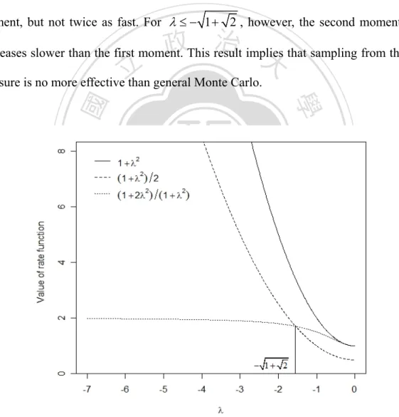
(44) Combining all results, we get the formulation.. 1 b 2 1 + 2λ 2 log E{( pˆ ET ) 2 } = − 2 ( ) m →∞ m ρ 1+ λ 2 lim. □. Note That Theorem 3.1 shows that the estimator is asymptotical optimal only in the case λ ≥ 0 . With − 1 + 2 < λ < 0 , the second moment decreases faster than the first moment, but not twice as fast. For λ ≤ − 1 + 2 , however, the second moment even. 政治大. decreases slower than the first moment. This result implies that sampling from the new. 立. measure is no more effective than general Monte Carlo.. ‧. ‧ 國. 學. n. er. io. sit. y. Nat. al. Ch. engchi. i Un. v. Fig. 3-4 Comparison of rate function under λ < 0 for a single homogeneous model.. 36.

(45) In the case λ < 0 , to eliminate the linear effect of Fm ( z ) , using exponential twist method with parameter Fm' (tm ) does not achieve the maximum utility. Review the properties of exponentially twisted procedure, we know that the maximal variance reduction occurs when parameter Fm' (tm ) makes the mean value of f * ( z | μ ; σ ; λ ) locate at the point tm . Consider ( μ ; σ ; λ ) = (0,1, λ ) and λ ≥ 0 , we have. M ' (t ) e tm z f ( z | 0;1; λ ) dz = Z m M Z (tm ) M Z (tm ) tm2 2. m. 1+ λ2. =. 2e Φ (. io. n. al. 1+ λ2. λ. 1+ λ2. → tm , if m → ∞. Ch. engchi U. λ. 1+ λ2. λ 1+ λ2. tm ). tm ). tm ). y. 1 + λ 2 Φ(. λ. 1+ λ. φ( 2. ‧. Nat. = tm +. λ. λ. m. tm2 2. φ(. tm2 2. 學. ‧ 國. 立. 政治λ 大 2t e Φ ( t ) + 2e. tm ). sit. −∞. z. er. ∫. ∞. v ni. (3.6). (3.6) show that the maximal utility will happen if we apply exponential twist method to factor. The phenomenon coincides with that GL suggest. However, if λ < 0 , the mean value of f * ( z | 0;1; λ ) is. ∫. ∞. −∞. z. M ' (t ) e tm z f ( z | 0;1; λ ) dz = Z m M Z (tm ) M Z (tm ). 37.

(46) φ(. |λ |. t ) 2 m + 1 λ = tm + 1 + λ 2 1 − Φ( | λ | t ) m 1+ λ2. λ. ≈. 1 tm 1+ λ2. (3.7). This equation holds because of φ ( x) /1 − Φ ( x) ~ x . Observe (3.7), we know that the algorithm is less efficient if λ is getting smaller. This result in (3.7) also corresponds with Fig. 3-4. Namely, negative λ incurs a width which makes the variance increase.. 政治大 In the next Chapter, we will tailor the algorithm to eliminate the effect from shape 立 ‧. ‧ 國. 學. io. sit. y. Nat. n. al. er. parameter λ .. Ch. engchi. 38. i Un. v.

(47) Chapter 4. The New Method for SN Factor. In Chapter 3, we know that asymptotical efficiency can not be achieved because the nonlinear behavior of Fm ( Z ) is non-negligible. This suggests that to obtain further variance reduction we need to address the other component of Fm ( Z ) . Glasserman et al (1999) attempted to use stratification technique to decrease variability except for linear part. Here, we completely limit ourselves to IS methodology to build an efficient algorithm. Our approach emphasizes on choosing density “form” of Z rather than. 政治大 general result in Chiang, Yueh, and Hsie (2007) (henceforth CYH) but for a different 立 shifting, scaling or exponentially twisting. In the next section, we begin with a more. ‧ 國. ‧. 4.1. 學. model.. Extension of CYH Importance Sampling Algorithm. y. Nat. sit. The key idea in CYH is to find a simple alternative characterization of default. n. al. er. io. event. To motivate the algorithm we take, observe the following proposition:. Ch. Proposition 4.1. engchi. i Un. v. Consider a single factor model where ci = 1 , bi = b and ρi = ρ ; Random variables Z and ε i follow SN (0,1, λ ) and SN (0,1, 0) respectively. Then the set {Lm > mq} is equivalent to the event {Z > H [ mq +1]} if H[ mq +1] is denoted as [mq + 1] th order statistics of {H i }im=1 , where. Hi =. b m − 1− ρ 2εi. ρ 39.

(48) Proof: Since. I {Lm > mq} = 1. ⇔ ∑ I { X i > b m} > mq i. ⇔ ∑ I {Z > i. b m − 1− ρ 2 εi } > mq ρ. ⇔ I {Z > H[ mq +1] } = 1. [ mq +1]. }.. □. 學. ‧ 國. Hence, the event {Lm. 政治大 > mq} is equivalent to the event {Z > H 立. Proposition 4.1 indicates a simple alternative characterization for the event. ‧. {Lm > mq} . It provides a simpler way to ensure that for every replication where the set. y. Nat. n. al. er. io. factor model as following. sit. we interest always takes place. By Proposition 4.1, we create an estimator of single SN. Ch. engchi. i Un. v. I {Lm > mq}Lr. (4.1). where Lr = 1− FZ ( H[ mq+1] ) denotes the likelihood ratio and FZ is the cumulative density function of Z . Clearly, (4.1) is not restricted to what the distribution of Z is. This means that the algorithm is allowed to general case. We will consider behavior of (4.1) in the following theorem. By analyzing the asymptotical performance, we can find a useful guideline for choosing appropriate IS density of Z .. 40.

(49) Theorem 4.1 Consider a single factor model where ci = 1 , bi = b , ρi = ρ and ( Z , εi ) follow the same distribution assumption in Proposition 1, then (4.1) has bounded relative error.. Proof: First, we exploit the result shown in Lucas et al (2003). Assume that S j is a latent variable which obeys the general factor model. 政治大. S j = g( f , εj ). 立. ‧ 國. 學. where f. is common factor, ε j is specific risk factor, and g (⋅, ⋅) defines the. ‧. functional form of the factor model. Lucas et al (2003) used the Theorem 12.13 of. Nat. n. al. er. io. sit. y. Williams (1991) and indicate that. a.s 1 n lim ∑ I {S j < s*}→P( S j < s* | f ) n→∞ n j =1. Ch. engchi. i Un. By the same argument as Lucas et al (2003), we then have. Lm a.s → E[ I { X i > b m}| Z ] m→∞ m lim. So, we have. 41. v.

(50) E[ I {Lm > mq}] → P( E[ I { X i > b m} | Z ] > q ) = P( Z >. b m −Φ−1 (1− q) 1− ρ 2 ) ρ. = 1− FZ (. b m −Φ−1 (1− q) 1− ρ 2 ) ρ. The second moment of (4.1) is written as (by Theorem 1.10 of Shao (1998) and Theorem 4.3.1 of Sen and Singer (1993)). 立. 學. ‧ 國. E[ I {Lm > mq}L2r ]. 政治大. = E[ I {Lm > mq}(1− FZ (( H i )[ mq+1] )) 2 ]. n. al. Ch. engchi. er. io. b m −Φ−1 (1− q) 1− ρ 2 + o(1) 2 )) ρ. sit. y. Nat. ≤ (1− FZ (. ‧. ⎡ b m − 1− ρ 2 (εi ) m−[ mq ] 2 ⎤⎥ ⎢ = E ⎢ I {Lm > mq}(1− FZ ( ) ⎥ ρ ⎢ ⎥ ⎣ ⎦. i Un. v. Therefore, we have. lim sup m→∞. Var ( I {Lm > mq}Lr ) E[ I {Lm > mq}]. E[ I {Lm > mq}L2r ] − E 2 [ I {Lm > mq}Lr ] = lim sup E[ I {Lm > mq}] m→∞ <∞. □. 42.

(51) The method works well for portfolio whose tail behavior is dominated by a “key” random variable. To show that the results have content, we give two specific examples. For the first example, consider the model. Xi =. ν (ρi Z + 1− ρi2 εi ) S. , i = 1, …, m. Here Z is a standard normal random variable, εi are i.i.d standard normal random. 政治大 1, we can find the set. variables, and S is chi-square distribution with r degrees of freedom. Applying the. 立. key idea behind Proposition. {S < ( H i )[ mq+1]} where. ‧ 國. 學. H i = (ρi Z + 1− ρi2 εi ) / b m . It is the simpler expression of {Lm > mq} . Note that the. ‧. sample of Z is generated from the original distribution. By a analogous algorithm in. sit. y. Nat. section 3.3, we get a efficient estimation of {Lm > mq} . In this model, the random. io. al. n. sufficient to achieve substantial variance reduction.. Ch. engchi. er. variable S plays a key role to vanish variability. Changing the measure of S is. i Un. v. Table 4-1：Comparison of different methods for m = 250 ; ν = 12 ; q = 0.25. .. P( Lm > mq ) Method. Algorithm 1. CYH Method. (Runs: 5×104 ). (Runs: 5×104 ). V .R. ρ. Prob. est. S .E. Prob. est. S .E. 0.1. 8.58×10−6. 1.63×10−7. 8.53×10−6. 1.36 ×10−7. 1.43. 0.2. 9.74 ×10−6. 1.85×10−7. 9.75×10−6. 2.04 ×10−7. 0.82. 0.3. 1.18×10−5. 4.13×10−7. 1.18×10−5. 3.18×10−7. 1.68. 0.4. 1.39 ×10−5. 8.61×10−7. 1.42 ×10−5. 4.93×10−7. 3.05. 43.

(52) Table 4-1 shows the performance of two estimators. Algorithm 1 is the suggestion of Bassamboo et al (2008) and we know that it has the bounded relative error. In the last column, we list the sample variance ratio V .R. V .R =. [ S .E ( p A1 )]2. 5×104 × 4 [ S .E ( p CYH )]2 5×10. 政治大. , where p A1 refers to the estimator of Algorithm 1 and p CYH refers to the estimator of. 立. CYH method. We find the fact that p A1 and p CYH have analogous performance of. ‧ 國. 學. simulation in Table 4-1. But, note that the implementation of the new method is more. ‧. easily.. sit. y. Nat. io. al. er. The next example illustrates the normal case discussed in Glasserman (2004). All. n. obligors are divided into two blocks. The first block consists of m1 obligors whose. Ch. engchi. i Un. v. marginal default probability is p1 . This block is dominated by the factor Z1 and has a common loading a1 . The second block comprises the last m − m1 obligors. All obligors in the second block have marginal default probability p2 and affected only by factor Z 2 with a common loading a2 . This model is. X i = a1Z1 + 1 − a12 ε i , i = 1,… , m1 X j = a2 Z 2 + 1 − a22 ε j , j = m1 + 1,… , m. 44.

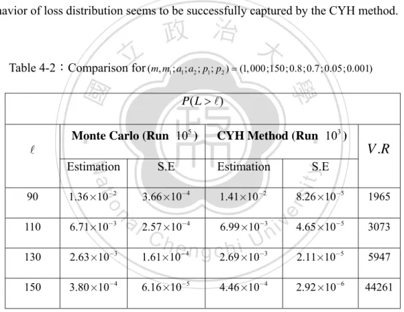
(53) m1. Set N1 = ∑ I { X i > Φ −1 (1 − p1 )} and N 2 = i =1. then is written as. ∪E. i,. m. ∑. j = m1 +1. I { X j > Φ −1 (1 − p2 )} , the equivalent set. where Ei , = {( z1 , z2 ) | N1 + N 2 ≥ , N1 = i} .. i. Table 4-2 shows the performance of general Monte Carlo and the CYH method. Note that variance reduction is measured relative to general Monte Carlo simulation. The CYH method provides an excellent performance than general Monte Carlo. The behavior of loss distribution seems to be successfully captured by the CYH method.. 立. 政治大. 學. P( L > ). CYH Method (Run 103 ). ‧. Estimation. 90. 1.36 ×10−2. 3.66×10−4. 1.41×10−2. 110. 6.71×10−3. 130. 2.63×10−3. 150. 3.80 ×10−4. V .R. S.E. y. S.E. Nat. Estimation. io. sit. Monte Carlo (Run 105 ). 8.26 ×10−5. er. ‧ 國. Table 4-2：Comparison for (m, m1 ; a1 ; a2 ; p1 ; p2 ) = (1, 000;150; 0.8;0.7; 0.05;0.001). n. a l 2.57 ×10 6.99 ×10 i v 4.65×10 n Ch U i e h n c g 1.61×10 2.69 ×10 2.11×10. 1965. −4. −3. −5. 3073. −4. −3. −5. 5947. 6.16 ×10−5. 4.46 ×10−4. 2.92 ×10−6. 44261. Although using order statistic increases simplicity, the flexibility is restricted simultaneously. For instance, if all the exposures ci are different from each other, then the sorting and partitioning procedures make the method time consuming. Obviously, the original problem in estimating rare event is transferred into another one. For more discussions about determination of key random variable is referred in Lucas et al (2003). 45.

(54) 4.2. The Proposed algorithm for Skew Factor Model Note the conclusion in Theorem 4.1, we know the likelihood Lr has an excellent. utility in variance reduction. Although the new method is inflexible to tackle inhomogeneous portfolio, it provides a way to build IS density for Z . In the following, we will introduce the strategy to search an effective IS algorithm.. Consider the result described in section 3.3, we know that vanishing linear. 政治大. variability of Fm ( z ) can increase the efficiency of simulation except for λ < 0 .. 立. ‧ 國. 學. Therefore, the procedure of eliminating the linear part of Fm ( z ) is essential. This means the new likelihood ratio LNew ( z ) = f ( z | 0;1; λ ) / f New ( z ) must contain the r. ‧. function exp(−tm z ) , namely. n. Ch. engchi. er. io. al. sit. y. Nat LNew ( z ) ∝ exp(−tm z ) r. i Un. v. (4.2). Furthermore, in the second part of Theorem 3.1, we find that the nonlinear behavior of Fm ( z ) seriously effect the efficiency of variance reduction. To eliminate this effect from the nonlinear part, we consider the limit regime rather than integral itself. We focus on modifying the other part of density of Z but for vanishing nonlinear part of Fm ( z ) directly. With the definition of asymptotically optimal, we need to find a likelihood ratio which decrease as fast as possible if we apply IS to Z .. In Theorem 4.1, Lr is of the bounded relative property. It is reasonable to utilize 46.

(55) asymptotical decay rate of Lr to create appropriate IS density. In multifactor and inhomogeneity case, however, getting a likelihood ratio like Lr is difficult. So we turn attention to setting where expectation of likelihood ratio decays in the same rate of Lr . In other words, we expect the following equation holds. log Lr =1 m→∞ log E[ LNew ( z )] r. (4.3). lim. 政治大. Once we find a new LNew ( z ) satisfying (4.2) and (4.3), the corresponding IS density is r. 立. then determined. Note that the combinative way leads to not only vanishing the linear. ‧ 國. 學. effect but considering the nonlinear part of Fm ( z ) simultaneously.. ‧. sit. y. Nat. To represent our procedure precisely, we consider the setting where. io. n. al. er. Z ~ SN (0,1, λ ) and λ < 0 . Clearly, it is difficult to directly calculate. ∞. Lr = ∫ b. Ch. m − 1−ρ 2 εi )[ mq+1] ρ. (. engchi. 2φ(t )Φ(λt )dt. i Un. v. If m is large sufficiently, an approximation for the integral (e.g, Shao 1998, Chap. 1 and Sen and Singer 1993, Chap. 4) suggests that. ∞. Lr ~ ∫ b. m +Φ−1 ( q ) 1−ρ 2 ρ. 2φ (t )Φ(λt )dt. 47.

(56) Therefore, for any small value δ , Lr is simplified into. Lr = 2δφ(tm + o( m ))Φ(λtm + o( m )). The last equation holds because of tm = O( m ) . This discussion of tm is shown in GL. N Then, the associated new IS density f New is written as. N f New ( z ) = φ ( z − tm ). 立. 政治大. (4.4). io. = 2∫. n. al. ∞. −∞. exp(−tm z +. Ch. = 2 exp(−tm. y. φ( z )Φ(λ z ) φ( z − tm )dz φ ( z − tm ). sit. Nat. −∞. tm2 )Φ(λ z )φ( z − tm )dz 2. er. ∞. E[ LNew ( z )] = 2∫ r. ‧. ‧ 國. 學. Note that the choice of IS density makes E[ LNew ( z )] satisfy (4.3), that is r. i Un. v. e ntg) +c th)i Φ(λ(ξ + t (ξ + 2 m. m. 2. m. )). ~ Lr. where ξ denotes a constant. The last equation holds because of the second mean value theorem for integral. Note that the choice of an appropriate IS density in such procedure is not unique. For instance, the following density. N f New ( z ) = 2φ( z − tm )Φ(| λ | ( z + tm )). 48.

(57) is another feasible one. By the similar argument, a appropriate IS density for λ ≥ 0 is. P f New ( z) =. 2 etm z φ( z )Φ(λ z ) M (t | 0;1; λ ). (4.5). P Especially, when λ = 0 , f New becomes the IS density GL suggest. For notational. simplicity, considering (μ, σ ) = (0,1) , we build our algorithm as following:. 1.. 立. Calculate tm = arg max{Fm (t ) − t 2 / 2} . t. ‧ 國. 學. 2.. 政治大. Check value λ of Z , choose (4.5) as IS density of Z if λ ≥ 0 and (4.4). ‧. otherwise.. Set tm to the IS density.. 4.. Sampling Z and calculate the product LNew ( z ) of each likelihood ratio. r. 5.. Compute θm ( z; q ) .. 6.. Return the estimate I {Lm > mq} Lr. n. al. er. io. sit. y. Nat. 3.. Ch. engchi. i Un. v. is the combined likelihood ratio. If we repeat step where Lr = e−θm ( Z ;q ) Lm +ψm ( θm ( Z ;q ), Z ) LNew r 1 to 6. times, an estimator pˆ New can be constructed by averaging the. values of. the estimates, we have a estimation for P ( Lm > mq ) under skew normal copula model. Once we have selected a new parameter vector tm which satisfies. 49.

(58) 1 tm = arg max{Fm (t ) − t T t} , 2 t. choosing (4.4) or (4.5) and component of tm for single IS density; we can easily extend the single factor to multiple factors.. 立. 政治大. ‧. ‧ 國. 學. n. er. io. sit. y. Nat. al. Ch. engchi. 50. i Un. v.

(59) 4.3. Asymptotic Optimality. We now consider the performance of the estimator pˆ New . The strength of our proposed lies in its variance reduction efficiency established by the following theorem:. Theorem 4.2 Consider the same assumption in Theorem 4.1, then (a) For λ ≥ 0 1 b2 lim log E[ I {Lm > mq}] = − 2 m →∞ m 2ρ. 立. 政治大. ‧. ‧ 國. (b) For λ < 0. 學. 1 b2 lim log E[( pˆ New ) 2 ] = − 2 m →∞ m ρ. 1 b 2 (1 + λ 2 ) log E[ I {Lm > mq}] = − m →∞ m 2ρ 2. n. al. Ch. engchi. sit er. io. 1 b 2 (1 + λ 2 ) log E[( pˆ New ) 2 ] = − m →∞ m ρ2 lim. y. Nat. lim. i Un. v. Proof: For λ ≥ 0 , the proof is the same as (a) in Theorem 3.1. We consider the part (b) directly.. (b): First we show that. lim inf m →∞. 1 b 2 (1 + λ 2 ) log E[ I {Lm > mq}] = − m 2ρ 2. By the similar argument in Theorem 3.1, we know for arbitrary τ > 0 51.

(60) E[ I {Lm > mq}] = P( Lm > mq | p ( Z ) = q + υ ) P( p( Z ) > q + υ ). 1 b m +Φ −1 (q + υ ) ) ≥ P( Z > ρ 2 ≥ φ( zm + τ )Φ(λ ( zm + τ )). where zm = {b m +Φ −1 (q + υ )}/ ρ . We have. 政治大. 1 1 lim inf log E[ I {Lm > mq}] ≥ lim inf log φ ( zm + τ ) m →∞ m m →∞ m. 立. ‧ 國. ‧ y. sit. al. n. m →∞. 1 b2 log φ ( zm + τ ) = − 2 m 2ρ. er. io. lim inf. 1 log Φ (λ ( zm + τ )) m. 學. m →∞. Nat. Note that. + lim inf. Ch. engchi. i Un. v. Applying the property φ( x) / Φ(−x) ~ x as x → ∞ , we get. lim inf m →∞. 1 −b | λ | φ (λ ( zm + τ )) log Φ (λ ( zm + τ )) = lim inf m →∞ m 2 ρ Φ (λ ( zm + τ )) = lim inf. −b | λ | φ (| λ | ( zm + τ )) 2 ρ m Φ (− | λ | ( zm + τ )). = lim inf. −b | λ | {| λ | ( zm + τ ) + o( m )} 2ρ m. m →∞. m →∞. 52.

(61) =−. bλ 2 2ρ 2. Next, we show. lim sup m →∞. 1 b 2 (1 + λ 2 ) log E[( pˆ New ) 2 ] ≤ − m ρ2. By the similar discussion in Theorem 3.1, we have. 立. 政治大. ≤ 4 E[exp{2 Fm ( Z ) − tm Z + tm2 }Φ 2 (λ Z )]. ‧. ‧ 國. 學. E[( pˆ New ) 2 ] = E[ I {Lm > mq} Lr2 ]. ≤ 4 exp{2 Fm (tm ) − tm2 }E[Φ 2 (λ Z )]. y. Nat. n. al. er. io. sit. ≤ 4 exp{2 Fm (tm ) − tm2 }E[Φ 2 (λ Z + λtm )]. Ch. i Un. v. Using the second mean value theorem for integral, for a small value ζ , we get lim sup m →∞. engchi. 1 1 log E[( pˆ New ) 2 ] ≤ lim sup {− zm2 (1 − ζ )} m m m →∞ + lim sup m →∞. =−. 1 log E[Φ 2 (λ Z + λ tm )] m. b2 1 + lim sup log Φ 2 (λtm + o( m )) 2 ρ m m →∞. Observe that. 53.

(62) lim sup m →∞. 1 2 log Φ 2 (λ tm + o( m )) = lim sup log Φ (λ zm + o( m )) m m m →∞ = lim sup m →∞. =−. −b | λ | {| λ | zm + o( m )} ρ m. b2λ 2. ρ2. Combining all the result and applying Jensen’s inequality we complete the proof.. □. 政治大. This result indicates that our proposed IS algorithm should be effective in estimating. 立. loss distribution. Even though the assumption in Theorem 4.2 is for homogeneous single. ‧ 國. 學. factor model, the proposed algorithm is practicably applied to multifactor and. ‧. inhomogeneity cases. Note that our proposed algorithm does not require what density the factor Z should follow. When the specific factors are of arbitrary distribution, we. y. Nat. al. er. io. sit. need only to modify the associated f New ( z ) to satisfy equation (4.3). In next chapter,. n. our numerical results for skew normal factor model also confirm the expectation.. Ch. engchi. 54. i Un. v.