利用整數型延伸式精簡基因演算法建造三維積體電路之直角史坦納樹

全文

(1)國立交通大學資訊科學與工程研究所碩士論文. 利用整數型延伸式精簡基因演算法建造三維積體電路之直角史坦納樹 Constructing the Rectilinear Steiner Tree in 3D ICs with Integer Extended Compact Genetic Algorithm. 研究生：李文瑜指導教授：陳穎平. 中華民國. 教授. 九十七. 年七月.

(2) 利用整數型延伸式精簡基因演算法建造三維積體電路之直角史坦納樹 Constructing the Rectilinear Steiner Tree in 3D ICs with Integer Extended Compact Genetic Algorithm. 研究生 : 李文瑜. Student : Wen-yu Lee. 指導教授 : 陳穎平. Advisor : Ying-ping Chen. 國立交通大學資訊科學與工程研究所碩士論文. A Thesis Submitted to Institute of Computer Science and Engineering College of Computer Science National Chiao Tung University in partial Fulfillment of the Requirements for the Degree of Master in. Computer Science. July 2008. Hsinchu, Taiwan, Republic of China 中華民國九十七年七月.

(3) Constructing the Rectilinear Steiner Tree in 3D ICs with Integer Extended Compact Genetic Algorithm Student : Wen-yu Lee. Advisor : Ying-ping Chen. Institute of Computer Science and Engineering College of Computer Science National Chiao Tung University. Abstract Rectilinear Steiner Tree (RST) has wide researches and applications in Very Large Scale Integrated (VLSI) circuit design. Generally, the RST is used to pre-estimate the circuit wire length before the VLSI routing stage, which is applied to interconnect different circuit components. Unfortunately, how to construct a RSMT is a NP-Complete problem. To make things worse, with the developing technology of Three-Dimensional Integrated Circuits (3D ICs), the complexity of the RST construction in 3D space is much higher than traditional RST construction, which only focuses on the two dimensional plane. Obviously, it is quite urgent to develop an effective way to construct a 3D RST. Therefore, the author presents the use of Integer Extended Compact Genetic Algorithm (iECGA), which can effectively solve highly complicated problems, to construct a 3D RST for 3D ICs. The experimental results show that the iECGA can effectively construct 3D RSTs in a reasonable time and outperforms than traditional Genetic Algorithm (GA). The author believes that the proposed strategy may be suitable for larger problems and can be extended to the problem of obstacle-aware 3D RST construction with in the future..

(4) 利用整數型延伸式精簡基因演算法建造三維積體電路之直角史坦納樹學生 : 李文瑜. 指導教授 : 陳穎平. 國立交通大學資訊科學與工程研究所. 中文摘要史坦納樹被廣泛的應用於現今超大型積體電路設計。一般而言，史坦納樹可以在積體電路繞線階段之前，利用來預估電路的繞線長度。然而，很不幸地，如何建構一個史坦納樹是一個 NP-Complete 的問題。而另一方面，隨著現今科技的發展，對於三維積體電路的需求日益增大，第三維度的導入，更加深了史坦納樹建構的複雜度，並且，過去用於二維積體電路的史坦納樹建構法並沒辦法良好地延伸至三維空間；因此，發展良好的三維史坦納樹建構法是相當有其必要性的。因此，作者使用整數型延伸式精簡基因演算法(iECGA)，用來解決此高複雜度的三維空間史坦納樹建構問題。根據實驗結果顯示整數型延伸式精簡基因演算法可以有效率地在合理的時間下，建構出良好的三維空間的史坦納樹；優於傳統的基因演算法(GA)。在未來的發展性，此研究未來可以進一步地發展於更複雜的問題，例如考慮具有障礙物的三維空間史坦納樹建構。.

(5) Contents Abstract Table of Contents List of Figures List of Tables 1. Introduction. 1. 1.1 The Three-Dimensional Rectilinear Steiner Tree……………………………...1 1.2 Previous Work…………………………………………………………………3 1.3 Motivation……………………………………………………………………..4 1.4 Our Contribution………………....………...………………….………………5 2. Problem Formulation. 6. 3. Previous Work 10 3.1 Preliminary…………………………………………………………………...10 3.2 The Deterministic Approaches for RST Construction …................................12 3.3 The GA-based 2D RST Construction ……………………………………….13 3.4 The GA-based 3D RST Construction ……………………………………….16 4. Algorithm and Design Flow 18 4.1 Evolutionary Algorithm (EA) ...………………………...…...………………18 4.2 Genetic Algorithm (GA) …………………………………….………………20 4.3 Chromosome Encoding ....……………………………………..……...…….21 4.4 Fitness Function ......…………………………………………………………22 4.5 Integer Extended Compact Genetic Algorithm (iECGA) .....………………..23 4.6 Design Flow ........……………………………………………………………32 5. Experiment Result 34 5.1 Experiment and Parameters…………………………………………………..34 5.2 Population Size Selection…………………………………………………….35 5.3 Solution Quality Analysis…………………………………………………….43 5.4 The Comparison between GA and iECGA …………………………………..46.

(6) 6. Conclusion 51 6.1 Summary of the thesis ...…………………….………………………….........51 6.2 Future work ...……………………………….…………………………….....52 6.3 Conclusion .....………………….........….....….……………………………...53 Bibliography. 54.

(7) List of Figures 1.1 A 4 pins rectilinear spanning tree and a 4 pins RST with 2 Steiner points .…….3 2.1 Five pins are distributed on 3D space, the complete graph of the five pins, the MST of the pins and a RST connects five ...…………………....………………..8 2.2 A RST respects to the objective function .....……………………………………9 3.1. An example of K5 ...……………………………………………………………11. 3.2. A graph consists of four vertices and five weighted edges ...………………….11. 3.3. An example of rectilinearization ………………………………………………15. 3.4. Two different ways to rectilinearize a slant edge ...……………………………15. 4.1 The pseudo code of the GA ...………………………………………………….21 4.2 Six possible combination for rectilinearizing a slanted edge ....……………….22 4.3. The overall ECGA flowchart ..……………………………………………........29. 4.4 The pseudo code of the ECGA .………………………………………………..30 4.5. The flowchart of our algorithm ………………………………………………..33. 5.1. Population size and tournament selection effect ………………………………36. 5.2. Comparisons between the solution quality and the population size .............38-42. 5.3. Comparisons between G(0) and iECGA ...…………………………………….44. 5.5 The cost reduction percentage of the iECGA for each problem size .…………45.

(8) 5.5. The cost reduction percentage for each problem size ....………………………48. 5.6. Comparisons between G(0), GA and iECGA ....……………………………….49. 5.7. Comparisons of the convergence rate between GA and iECGA ...…………….50.

(9) List of Tables 4.1. A four genes MPMs model example …….…………………………………….26. 5.1. The cost reduction percentage of iECGA for each problem size ..…………….46. 5.2. Comparisons between GA and iECGA ..………………………………………48. 5.3. Comparisons of the convergence rate between GA and iECGA ..……………..49.

(10) Chapter 1 Introduction In the first part of the chapter, Section 1.1, the 3D RST will be briefly introduced. Then, the author would like to roughly review the previous work in Section 1.2. Subsequently, the motivation of the thesis will be given in Section 1.3. Finally, the conclusion of this chapter will be shown in Section 1.4.. 1.1 The Three-Dimensional Rectilinear Steiner Tree Many techniques have been widely proposed to pre-estimate the circuit wire length before the practical routing stage, which is applied to interconnect different circuit components. One measure of circuit wire length is Half Perimeter Wire Length (HPWL). This method only measures the half perimeter of the bounding box which is a smallest rectangle to cover all the pins of a net to predict the wire length. Unfortunately, the method is too optimistic and often underestimates routing length.. 1.

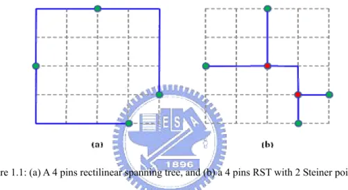
(11) Another way to estimate the wire length is Rectilinear Minimum Spanning tree (RMST). However, this method also cannot accurately estimate the wire length. Fortunately, the construction of Rectilinear Steiner Tree (RST) has been widely researched and provides a promising way to effectively pre-estimate the length of interconnect in the last decade. The concept of the RST is quite similar to the rectilinear spanning tree. Given a set of vertices, called as pins in VLSI terminology, a rectilinear spanning tree can span all the pins by vertical and horizontal line segments. In other words, the tree is composed of all the pins without any cycle, as shown in Figure 1.1(a). The difference between a RST and a rectilinear spanning tree is that the RST can introduce Steiner points, vertices with degree greater or equal to 3, to further reduce the wire length. That is, the rectilinear spanning tree is a special case of the RST. Therefore, the rectilinear spanning tree in Figure 1.1(a) is also a RST. Assume that the length and width for each grid are the same, 1 unit; the total wire length of the rectilinear spanning tree is 14 units. Obviously, it seems the wire length cannot be further reduced without adding any new Steiner points. In Figure 1.1(b), by appropriately adding two Steiner points (red vertices), the total wire length can be reduced to 8 units. This tree is a RST, not a rectilinear spanning tree anymore. The aforementioned RST is located in Two-Dimensional (2D) plane. In fact, in. 2.

(12) present System-on-Chip designs, people suppose to vertically stack multiple dies in a package, called Three-Dimensional Integrated Circuit (3D IC), in order to integrate more functions into a single chip and further decrease total wire length. The definition of 3D IC is a chip with two or more layers of active electronic components, integrated both vertically and horizontally into a single circuit. Therefore, it is quite necessary to extend the original 2D RST to 3D space; that is, 3D RST.. Figure 1.1: (a) A 4 pins rectilinear spanning tree, and (b) a 4 pins RST with 2 Steiner points.. 1.2 Previous Work However, how to construct a RST is a NP-Complete problem [1]. Although RST is a NPC problem, it is still worth researching because of its accuracy. Many prominent approximation approaches have been proposed. Griffith et al. [5] proposed a speedup implantation of RMST based on the Iterated-1 Steiner (I1S) technique. This heuristic approach can obtain a near-optimal solution in the polynomial time. On the contrary, an exact algorithm called GeoSteiner was implemented by Warme et al. [6]. After that,. 3.

(13) Chen et al. [7] developed an efficient heuristic approach called Refined Single Trunk Tree (RST-T), which can efficiently predict the net length of no more than 10 pins within 6% of the optimal solution. Furthermore, Zhou [8] provided an O(nlogn) RST algorithm based on the spanning graph and the sequentially a fast table lookup technique was presented by Chu [9]. However, the aforementioned previous work only focuses on 2D plane. Obviously, the 3D RST is more complex and difficult than the 2D case.. 1.3 Motivation In order to effectively address the complex problem, the author has observed that the Genetic Algorithms (GAs) have been successfully applied to many NPC problems and can get an excellent result. For RST, the GAs first applied to the RST problem in 2002 [10]. Julstrom solved the RST problem through extend coding of spanning trees to specify Steiner point choices for the spanning trees to minimize the total wire length. Afterwards, Kanemoto et al. [12] extended the previous work and considered the RST for 3D ICs. They claimed that their algorithm can get a good RST in 3D space. Although the aforementioned researches can apply the GAs to 2D or 3D RST problems and get a good result. However, their method only can solve small problem.. 4.

(14) For large problems, the runtime of their methods may be too long and cannot get a feasible result in a reasonable time. The reason may be because that the performance on large instances with GA is not very wellness. Therefore, it only can adapt to solve small problem, not suitable for large problems. Based on this observation, the author would like to improve the previous work and develop an effective and efficient to construct a 3D RST.. 1.4 Our Contribution In this thesis, the author proposes the use of Integer Extended Compact Genetic Algorithm (iECGA), which can effectively solve highly complicated problems, on construction a 3D RST for 3D-IC designs. The experimental results show that the iECGA can effectively construct 3D RSTs in reasonable time and outperforms than traditional GAs. The remainder of the thesis is organized as follows. In Chapter 2, we would like to formulate the 3D RST problem formally. Then, the previous work will be reviewed in Chapter 3. Subsequently, the Chapter 4 will elaborate our iECGA. Finally, the experimental results and the conclusion will be described in Chapter 5 and Chapter 6, respectively.. 5.

(15) Chapter 2 Problem Formulation Here, we formulate the 3D RST formally. Given a set of pins P = { p1 ,p2, p3,….,pn } on 3D spaces, each pin pi has coordinate location (xi, yi , zi ), where xi and yi represent pin location on a plane exactly as traditional 2D chips, the zi denotes which routing layer this pin lies on. Our objective consists of two parts: 1) interconnection cost and 2) maximum propagation time. For the first part, since the vertical-connection (via) cost is larger than the horizontal-connection one, we multiply a factor Cv to the vertical length to emphasize the cost of the vertical-connection, as shown in equation (1). Φ(L) = Σx_l +Σy_l + Cv *Σz_l,. (1). where Φ(L) is cost of the wire length, and x_1, y_1, and z_1 represent the wire length in x-direction, y-direction, and z-direction, respectively. For the second part, the maximum propagation time can be estimated by the maximum distance between two. 6.

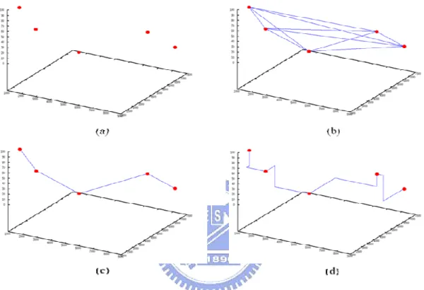
(16) pins on the tree. Since the unit between the interconnection cost and propagation time cost is different, these two terms should be normalized and then could be considered in the equation, as shown in equation (2). Φ = Cw* Φ(L) + Ct* Φ(T),. (2). where Φ and Φ(T) indicate the overall cost and the cost of the maximum propagation time. The proposed algorithm should construct a 3D RST and minimize the overall cost. Here shows an example to illustrate this problem. Generally, the problem input is a number of pins, five pins in our example, distributed on 3D space, as shown in Figure 2.1(a). The goal of the problem is to connect all the pins through proper Steiner points’ generation and forms a RST with the objective function consideration. This scene can be illustrated as Figure 2.1(d). Generally, the basic steps to solve this problem can be illustrated as follows. First, construct a complete graph for the five pins, as shown in Figure 2.1(b). Second, the Minimum Spanning Tree (MST) can be extracted from this graph, as shown in Figure 2.1(c). Note that the total wire length of the MST is calculated based on the Manhattan distance, not the Euclidean distance. In addition, the edges of the MST are slant, not rectilinear ones. Finally, through proper optimization strategies, the slant edges can be rectilinearized and generate the final RST, as shown in Figure 2.1(d). Note that different objective functions may lead to. 7.

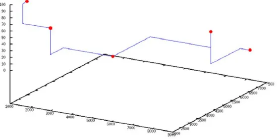
(17) different RSTs. The Figure 2.2 shows a RST respecting to our objective function. Most of the previous work are focused on the final step and change the optimization strategy. The next chapter will review the previous work more detailed.. Figure 2.1: (a) Five pins are distributed on 3D space. (b) The complete graph of the five pins. (c) The MST of the pins. (d) A RST connects five pins.. 8.

(18) Figure 2.2: A RST respects to the objective function.. 9.

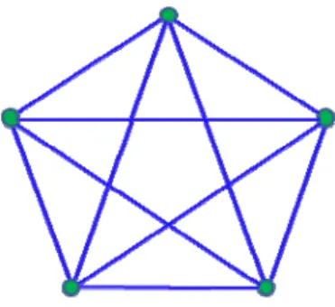
(19) Chapter 3 Previous Work In this chapter, the previous work is reviewed. First, to facility the explanation, the construction of complete graph and MST are roughly reviewed in Section 3.1. Second, Section 3.2 presents some general deterministic strategies for RST problem. Third, Section 3.3 introduces some prior researches based on the GA, which are non-deterministic methods, for common 2D RST problem. Finally, the GA-based 3D RST construction algorithm is described in Section 3.3.. 3.1 Preliminaries 3.1.1 Complete Graph Construction A complete graph is a simple graph in which every pair of distinct vertices is connected by an edge. Therefore, the complete graph on n vertices have overall n*(n-1)/2 edges with each vertex connected to other (n-1) vertices and denotes by Kn.. 10.

(20) Figure 3.1 illustrates an example of K5. Given five vertices, the complete graph of these vertices contains overall ten edges.. Figure 3.1: An example of K5.. 3.1.2 Minimum Spanning Tree (MST) Construction Given a connected undirected graph, a spanning tree of that graph is a subgraph which is a tree and connects all the vertices together. A single graph can have many different spanning trees. Generally, each tree edge can be assigned a weight which is a number representing how unfavorable it is, and the spanning tree with minimum weight sum is called the MST. Note that the MST may not be unique.. Figure 3.2: (a) A graph consists of four vertices and five weighted edges. (b) The MST of (a).. The reason why many prior researches tended to construct a MST before practically generating an optimal RST is that they attempted to provide a “good enough” solution. 11.

(21) to their heuristic algorithm engine. In other words, they believe that a good “guess” is much important to this problem. The “guess” is according to the well-known property, cost (MST (P))/ cost (MRST (P)) <=3/2 [5]. That is, the MST is a fairly good approximation to the minimum RST [2].. 3.2 The Deterministic Approaches for RST Construction To date, there are many research efforts have been dedicated to the development of deterministic algorithms for RST construction. Among these works, Zhou’s spanning graph based RST construction strategy [8] and Chu’s lookup table based RST construction strategy [9], particularly draw much attention. Therefore, let us focus on these two works. In Zhou’s work, a worst case running time of O (nlogn) efficient RST construction algorithm was developed [8]. This work is based on a spanning graph which can retain the ideal Steiner tree and simultaneously reduce the solution space. In other words, the optimal solution still exists on the spanning graph. After building a spanning graph, the proposed algorithm effectively consider the connection of nearby edges and deletion of longest edges to avoid the cycle formation. Finally, the resulting RST can be obtained. In Chu’s work, a lookup table based strategy was proposed [9]. The underlying idea. 12.

(22) of this approach is to pre-compute the basic problem structures and record the corresponding results into a lookup table for future use. Once the simple problem structure is met, the result can be efficiently obtained. If the complex problem structure is met, the complex problem structure can be decomposed into several basic problem structures and efficiently solve. Then, the individual result of the basic problem structures can be merged to overcome the original problem. Obviously, this is a divide-and-conquer based strategy. The runtime of this work is quite fast. In addition, this method can also obtain high quality solution.. 3.3 The GA-based 2D RST Construction Since the nature of the RST construction is NP-Complete. To date, no one can find any deterministic algorithm to efficiently solve this kind of problems. Therefore, many researchers prefer to solve this kind of problems based on GAs, which are non-deterministic methods, providing the chance to efficiently address the NP-Complete problems. The development of the GA-based RST construction algorithms can trace back to the early days of Julstrom’s research [27]. This work encodes the underlying spanning trees by Prüfer numbers. The binary symbols are adapted to indicate the Steiner point choices and then generate a genetic coding for RST. However, this work inevitably. 13.

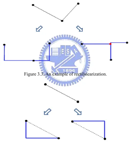
(23) leads to bad performance. What’s worse, the quality of the final result is not good enough even though the problem size is small. Afterwards, Palmer and Kirshenbaum proposed a new representation for trees in GA [28] and then Julstrom et al. extended this representation for RSTs [26]. Subsequently, Julstrom encoded the RST as lists of spanning tree edges with corresponding Steiner points [29]. Recently, Julstrom artfully circumvented the large solution space of the RST and focus on the Steiner point assignment [10]. This work dramatically reduced the search space for a good RST. Here, let us review this work more detailed. A RST composed of points on the 2D plane can be derived from a spanning tree by choosing Steiner points. The aim of this work is to seek a RST with near-shortest wire length on the given pins. Through properly observation, the author reduced the solution space of the original problem to the space of the spanning trees on given pins product the space of Steiner point choices for spanning tree edges. For clarity, please focus on an example shown in Figure 3.3. Given a spanning tree with slant edges, it is necessary to rectilinearize the edges to horizontal edges and vertical edges. If the left-bottom one is chosen, the total wire length is large. Nevertheless, if the right-bottom one is chosen, the total wire length can be reduced by introducing a Steiner point. Therefore, given a slant edge, the author defined two different ways to rectilinearize this edge as shown in Figure 3.4. In other words, two L-shape can be. 14.

(24) chosen. Therefore, each edge can be encoded to a bit. By applying the GA, the author can obtain a RST with minimal total wire length. The overall flow can be described as follows. Given the pins, the author first constructs a MST. Then, the author encodes all the edges of the spanning tree as binary strings. After that, the conventional genetic operators, two-point crossover and position-by-position mutation, can be applied to search the RST with minimal total wire length.. Figure 3.3: An example of rectilinearization.. Figure 3.4: Two different ways to rectilinearize a slant edge.. The experimental results show that this method can effectively get good, though never optimal RSTs. In addition, the performance of this method is reasonable even though the problem size is reach to 500 pins.. 15.

(25) 3.4 The GA-based 3D RST Construction Afterwards, Kanemoto et al. extends the previous research which only considered the 2D RST to 3D space and further considers the diameter in 3D VLSI layout design [12]. Note that the diameter refers to the longest routing path between all pins on a RST in this work. Similar to the previous research, the complete graph is constructed first. Then, the Euclidean MSTs for the given pins on the space can be extracted. Note that there may be several MSTs with the same total wire length. At this time, a tree with minimum diameter is chosen among the Euclidean MSTs. After that, the GA is applied to minimize the total wire length and the diameter, and finally, each edge segment of the Euclidean MST can be replaced by one of the six permutations of three segments which are parallel to the X-axis, Y-axis, Z-axis, respectively. To verify the effectiveness of the work, the author tested their algorithm on ten test data. The smallest problem size is 5 pins and the largest one is 14 pins. The experimental results showed that the adoption of GA for 3D RST construction is very effective when the problem size is small. However, the work is only suitable for smaller problem size. Intuitively, the efficiency of the program may deteriorate for larger cases. Therefore, new methodology should be proposed to overcome this problem. This demand exposes the motivation of this thesis. In this chapter, we roughly review the previous work. On one hand, the. 16.

(26) deterministic approaches can solve the RST problem in reasonable time. However, there is still much room for improvement on these techniques. On the other hand, the non-deterministic approaches provided another way to search a good RST. Nevertheless, these approaches may suffer from large runtime. In this thesis, we would like to improve the previous non-deterministic approaches and efficiently obtain a good solution. The detail of our approach is shown in the next chapter.. 17.

(27) Chapter 4 Algorithms and Design Flow In this chapter, we will introduce our algorithm for RST construction problem. First, the Evolutionary Algorithm and Genetic Algorithm are described in Section 4.1 and Section 4.2, respectively. Nest, Section 4.3 introduces how to encode input pins to genotype which is what we need to feed in our algorithm. Then, Section 4.4 establishes our fitness function. After that, Section 4.5 details our method. Finally, Section 4.6 presents our overall design flow.. 4.1 Evolutionary Algorithm (EA) In this section, the concept of the Evolutionary Algorithm (EA) and how it can be applied on real world problems are concisely described. The EA, which is a generic population-based meta-heuristic optimization algorithm, is a concept of algorithms originated from the evolutionary computation, which is a subfield of artificial. 18.

(28) intelligence that involves combinatorial optimization problems in computer science. Generally, EAs are search methods that take their inspiration form natural selection and survival of the fittest in the biological world. Basically, the EA ingeniously uses some mechanisms according to the biological evolution: reproduction, selection, mutation, and recombination. In a population, each individual represents a candidate solution to the optimization problem. To identify which individuals are better and which individuals are worse, the fitness function can be defined. The fitness function determines the environment within which the solutions are fitted or not. The higher the fitness value evaluated from the fitness function, the more suitable the individual is. Evolution of the population then takes place through the repeated application of the above operators. EAs consistently obtain well approximating solutions to all types of problems because they do not embed any assumption about the underlying fitness landscape; this generality can be shown by successes in fields as diverse as engineering, art, biology, economics, marketing, genetics, operations, research, robotics, social sciences, physics, and chemistry. In addition, apart from their use on the mathematical optimizers, the EAs have also been used as an experimental framework within which to validate theories about biological evolution and natural selection, particularly through work in the field of artificial life.. 19.

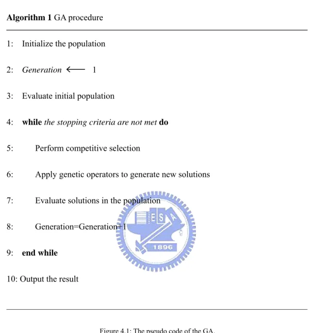
(29) 4.2 Genetic Algorithm (GA) To date, most people believe that the GA was initially conceived by Holland by means of studying adaptive behavior and it has largely been considered as function of optimization methods nowadays [11]. GA was proposed based on the concept of natural selection. Mainly, the operators of the GA contain selection, crossover, mutation and replacement. Initially, the population is composed of random generated individuals. These individuals form the first generation. In each generation, the fitness of every individual of the population is evaluated. Then, multiple individuals are stochastically selected from the current population based on their fitness values. After proper crossover and mutation, the replacement operator will be performed to form a new population. These procedures finish a generation and then the new population can be used in the next iteration of the algorithm to form next generation. Commonly, the algorithm terminates when either a given maximum number of generations has been achieved, or a satisfactory fitness level has been reached for the current population. Note that if the algorithm has terminated due to a maximum number of generations has been achieved, the satisfactory solution cannot be guaranteed. Figure 4.1 demonstrates the pseudo code of the GA.. 20.

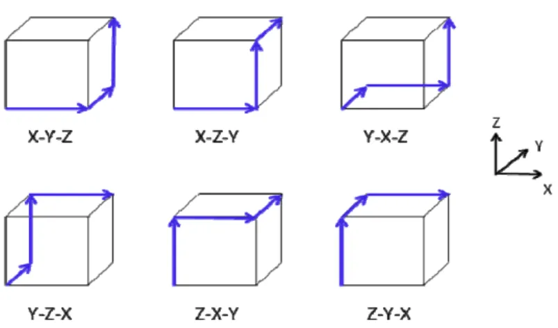
(30) _____________________________________________________________________ Algorithm 1 GA procedure 1: Initialize the population 2:. Generation. 1. 3: Evaluate initial population 4:. while the stopping criteria are not met do. 5:. Perform competitive selection. 6:. Apply genetic operators to generate new solutions. 7:. Evaluate solutions in the population. 8:. Generation=Generation+1. 9:. end while. 10: Output the result _____________________________________________________________________ Figure 4.1: The pseudo code of the GA.. 4.3 Chromosome Encoding In this section, we would like to introduce the chromosome encoding method in our work. The encoding method is similar to the previous work [12]. For each slanted edge of the MST, there are six possible orientations can be chosen, as shown in Figure. 21.

(31) 4.2.. Figure 4.2: Six possible combination for rectilinearizing a slanted edge.. Obviously, these orientations include all possible routing topology for rectilinearizing each slanted edge. Therefore, each gene of a chromosome can be an integer value range from 0 to 5 to represent one of the six orientations for each MST edge. Certainly, each chromosome is composed of (n-1) genes if the number of input pins is n.. 4.4 Fitness Function As mentioned earlier in Chapter 2, the objective of this thesis is to construct a RST with the interconnection cost and the maximum propagation time minimization. Therefore, for total wire length estimation, the slanted edges are transformed into three rectangular edges similar to the normal methods. Then, based on the equation (1) of the Chapter 2, the interconnection cost induced from the wire length can be computed. Note that there may be some edges are overlapped and the overlapped 22.

(32) length must be calculated at most once. Subsequently, the maximum propagation time can be computed by performing the well-known Breath-First Search algorithm for each pin and then pick the maximum length of the routing path. After that, the maximum propagation time can be estimated based on the linear model which assumes time is linear proportional to distance. After that, the interconnection cost and the maximum propagation time can be combined together based on the equation (2) of the Chapter 2. Hence, we defines the fitness function is the inverse value of the equation (2) of the Chapter 2. Note that the coefficients of this equation are used for normalization and weight.. 4.5 Integer Extended Compact Genetic Algorithm (iECGA) 4.5.1 Linkage Problem Since the GA was proposed, the importance of Building Blocks (BBs) [16] and their role in the working of GAs has long been recognized. By BBs, partial solutions of a problem are meant. In most situations, a problem could be divided into smaller sub-problems. Under this hypothesis, the problem solutions could be decomposed into some little parts, each of them is named “Building Block”. However, BBs are often destructed by the crossover operation during the GA processing. Based on this description, we could conclude that if the algorithm can. 23.

(33) correctly identify BBs and mix all BBs without any disruption, it can be expected that the good solution may be obtained very fast by merging the good BBs. The problem of the BB disruption is often referred to as the “linkage problem” [18].. 4.5.2 Extended compact genetic algorithm (ECGA) In order to enhance the ability of the sub-solution identification into the crossover and mutation operators in GAs, Estimation of Distribution Algorithms (EDAs) are proposed and developed by utilizing probabilistic models to capture and reflect the problem structure [22]. Compact Genetic Algorithm (cGA) is one kind of the EDAs. The cGA is a robust and efficient GA that possesses linkage learning ability. To enhance the ability of the cGA, the Extended Compact Genetic Algorithm (ECGA) was initially proposed by Harik [13] based on the cGA. The underlying idea of ECGA is that the ECGA tends to choose a good probability distribution to progress; this concept is equivalent to linkage learning. Therefore, ECGA has two important contentions should be concerned: one is how to select a “good” probability distribution; the other one is how to learn a genetic linkage. To explain how ECGA deals with these two concerns, it is essential to introduce the probability model for ECGA first. Then, how to evaluate a probability distribution will be described. Finally, an example will be given to. 24.

(34) demonstrate how ECGA select a “good” probability distribution and learn a genetic linkage. For ECGA, Marginal Product Models (MPMs) have been known to be a class of probability models used in probability distribution of ECGA. The underlying idea of MPMs is to divide the gene or variables into several linkage groups, which are mutually independent with each other, and then specify marginal probabilities for each linkage group. That is, MPMs are formed as a product of marginal distributions on a partition of the genes and are similar to those cGA and PBIL [15, 19, 20], except that they can represent the joint probability distribution over more than one gene at a time. Following is an example of the MPM to explain what it is and how it works. As shown in Table 4.1, the following MPM of a four-bit problem consists of three linkage groups [19]. Each linkage group maps to a gene partition. This model shows that the 1st and 3rd genes are linked together, but are independent to the other two genes. Moreover, the 2nd and 4th genes are independent to each other. In addition to the relationship specification, an MPM also specifies the marginal probabilities for each linkage group. Note that in this table, Xi means the value of the ith gene, and the symbol, P, represents to the marginal probability. This marginal probability can be computed based on the allele occurrence ratio of different patterns in past populations.. 25.

(35) Table 4.1: A four genes MPMs model example.. Group [1, 3]. Group [2]. Group [4]. P(X1=0, X3=0). P(X2=0). P(X4=0). P(X1=0, X3=1). P(X2=1). P(X4=1). P(X1=1, X3=0) P(X1=1, X3=1). Generally, the measure of a good distribution can be quantified by Minimum Description Length (MDL) models. MDL models can be used to identify MPMs quality and define the model complexity and the compressed population complexity of a probability distribution. Obviously, suppose that all the given conditions are equal, simpler distributions are better than complex ones. The identification of MPMs in every generation can be formulated as a constrained optimization problem. The definition of the combined complexity (Cc) is. Cc= Cm + Cp. where Cm is the model complexity which represents the cost of a complex model and Cp is the compressed population complexity which represents the cost of using a simple model as against a complex one. Obviously, the combined complexity is the summation of the model complexity and the compressed population complexity. The detail of the model complexity and compressed population complexity is shown in 26.

(36) following two equations.. m. Model Complexity (Cm) = log2 N ∑ 2 Si i =1. Compressed Population Complexity (Cp) = N. m. si. ∑∑ − p i =1 j =1. ij. log pij. where N is the population size, m is the number of groups (BBs), Si is the length of chromosome of each group. There are some basic assumptions in these two equations. Given a problem, it is assumed that this problem can be partitioned into “m” groups with each group has its size Si, i=1…m. The overall problem size is certain the summation of the size of total m groups. As for Pij, it is the number of chromosomes in the current population possessing bit-sequence; in other words, it is the frequency of the jth possible partial solution to the ith variable subset observed in selection population. After introducing the probability model and the evaluation model, we would like to give an example to demonstrate how ECGA select a “good” probability distribution and learn a genetic linkage as follows. Given a binary coding problem which length is L and its genes are independent, the problem can be partitioned into independent sub-problems in the initial building process of the MPM model as shown below.. 27.

(37) [0][1] …. [L-2][L-1]. Then, we try to merge each pair of groups to form a new MPM. The candidates can be shown as follows.. [0, 1][2] … [L-2][L-1], [0][1, 2] …. [L-2][L-1], …. [0][1] … [L-2, L-1]. The combined complexity of each produced MPM is computed, and then these combined complexities including the original one are compared. After that, the MPM with smallest combined complexity can be obtained. For example, if a MPM, [0, 1] … [L-2][L-1], has the smallest complexity, group [0] and group [1] can be combined into a new group [0, 1]. This above procedure continues until there is no way to further reduce the complexity, and then the procedure terminates. Finally, a MPM represents the linkage between genes can be obtained. Here, the overall ECGA flowchart and the pseudo code of ECGA are described in Figure 4.3 and Figure 4.4, respectively. As can be seen, the procedure of ECGA is quite similar to traditional GA. The ECGA also have the procedures of population initialization, fitness evaluation, parent selection and crossover. The most difference. 28.

(38) between ECGA and traditional GA is that the parent selection of ECGA is based on probability distribution and then uses the MPM to find genes linkage relationship. Note that the BBs of ECGA do not break in crossover step. Therefore, the evolution speed of ECGA is expected to be faster than traditional GA and coverage to the high quality solution.. Figure 4.3: The overall ECGA flowchart.. 29.

(39) _____________________________________________________________________ Algorithm 2 ECGA produce. 1: Random generate individuals 2: Generation. 1. 3: while the stopping criteria are not met do 4:. Calculate fitness values of individuals. 5:. Perform tournament selection. 6:. Use MPM to build a joint probability distribution. 7:. Use the generated MPM to perform crossover. 8:. Generation=Generation+1. 9: end while 10: Output the result Figure 4.4: The pseudo code of the ECGA.. 4.5.3Integer Extended compact genetic algorithm (iECGA). The aforementioned ECGA encodes the genes into real numbers. However, we need to encode genes into integers due to six orientations, as mentioned in Section 4.4. Therefore, the original ECGA can be restricted into integer domain, called Integer Extended Compact Genetic Algorithm (iECGA). The most different between ECGA. 30.

(40) and iECGA is that all genes of iECGA are represented as integers, not real numbers. Based on the aforesaid standpoint, a chromosome of iECGA is an integer vector, instead of a bit vector of the original ECGA. In addition, the MPMs and MDL criterion are modified to fit new representation [14]. In fact, the implementation of the MPM is a counting process in ECGA. For iECGA, the MPM also has to count the occurrence of all possible patterns [14]. To this end, we can assume that the range of genes value are from lower bound l to upper bound u, and the cardinality is d = u - l+ 1. There are d|s| patterns of a group with gene size |s|. Therefore, it is necessary to count all d|s| patterns before building the MPM of iECGA. For the MDL model of iECGA, the formula of the complexity has to be modified. Considering the iECGA, there are two criteria of a good distribution. One is the small model representation, and the other one is small population representation. Both of the criteria can be applied to integer vectors. As shown below, the base number in the formula of the model complexity is changed from 2 to k, but the compressed population complexity is unchanged.. m. Model Complexity (Cm) = logk N ∑ k Si i =1. Compressed Population Complexity (Cp) = N. m. si. ∑∑ − p i =1 j =1. 31. ij. log pij.

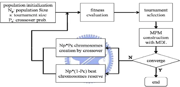
(41) Except the MPMs and the formula of model complexity, the rest parts of iECGA are the same as ECGA. Therefore, the iECGA can be conveniently applied to the 3D RST problem and produces a feasible solution.. 4.6 Design Flow Figure 4.5 shows our overall design flowchart. Given a 3D chip information and input pins information, including the 3D chip size, number of pins, and pins’ locations, the proposed algorithm first builds a complete graph to connect all the pins with each other as we described in Section 3.1.1. Then, the well-known Kruskal algorithm will be performed to extract a MST from the complete graph. Note that the concept of the MST is shown in Section 3.1.2. Finally, the kernel algorithm, iECGA will be applied to obtain a feasible RST to minimize the total wire length and maximum propagation time.. 32.

(42) Figure 4.5: The flowchart of our algorithm.. Before introducing the iECGA, it is instructive to give a preliminary introduction. Therefore, we would like to introduce the Evolutionary Algorithm and Genetic Algorithm in the following sections. Subsequently, we would like to show our encoding method and the fitness function. After all the knowledge is provided, the kernel algorithm, iECGA, will be described.. 33.

(43) Chapter 5 Experimental Results In this chapter, the author first describes our experimental conditions and the parameter setting in Section 5.1. Then, Section 5.2 explores how to find the most suitable population size for any given 3D RST problem. Subsequently, Section 5.3 shows the solution qualities of the generated 3D RSTs for all test cases. Finally, Section 5.4 compares this work and the previous work.. 5.1 Experiments and Parameters The program was written in C++ programming language and performed on an Intel Quad-Core CPU 2.4 GHz machine with Linux workstation. To demonstrate the power of our approach, we would like to compare our approach with the previous work [12]. Therefore, similar to [12], we initially generated ten test cases and the number of input pins is distributed from 5 to 14. However, this kind of problem sizes is too small. 34.

(44) to satisfy the demand of current IC design. Hence, it is worth to enlarge the problem size. In other words, to generate test cases with more input pin number. Therefore, we added three more test cases which have 50 pins, 100 pins, and 350 pins, respectively. For these test cases, each gene of the GA [12] and the iECGA was encoded into an integer distributed from 0 to 5 to represent one of the six orientations as mentioned earlier. The fitness function was discussed in Chapter 2 and Chapter 4 before. Hence, it can be skipped here. Moreover, the remainder parameters of the GA are unchanged to respect the previous work. For the setting of the remainder parameters of the iECGA, adaptive parameters are applied. The maximum generation of the iECGA is set to be 30 for small problem size (<= 14 pins) and 50 for large problem size (50 pins, 100 pins, and 350 pins). The parameter setting of the population size is discussed in Section 5.2. For the selection strategy, an elite strategy, tournament selection, was adapted. Note that the tournament size of the tournament selection is set to be 12, 14, or 16. Furthermore, the crossover rate is set to be 0.975000; that is, 97.5%.. 5.2 Population Size Selection In this section, the author presents how to choose an appropriate population size of a 3D RST problem. Figure 5.1 shows an illustration. The horizontal axis refers to different problem sizes and the vertical axis represents the population size.. 35.

(45) Figure 5.1: Population size and tournament selection effect.. Note that each experiment repeats 50 times and takes the average value to reduce the noise. In the experiments, the author would like to identify the smallest population size which is large enough to get the minimal cost, or maximal fitness value, for each test case. To reduce the complexity, the author focuses on the small test cases (<= 14 pins) and only considers 12, 14, and 16 to be the tournament size. This parameter is based on the experience. Moreover, the initial population size is set to be 50 units and then increases the step by 50 units. If the cost cannot be further reduced, the population size can be fixed. Therefore, each test case can record three optimal population sizes.. 36.

(46) It should be notice that most of the test cases can be effectively solved when the population sizes are between 50 and 150. Furthermore, using the tournament size 14 or 16 is more stable in the 3D RST problem. To be more detailed, the author shrinks the scale of the population size and observes the relationship between the 3D RST solution quality/cost and the population size. Here, the author sets the population size between 10 and 100 and increases the step by 5 units or 10 units. That is, the scale of the population size is 10, 15, 20, 25, 30, 40, 50, 60, 70, 80, 90, and 100, respectively. The experimental results can be shown in the sequential ten figures, Figure 5.2 (a)-(j). In these figures, the horizontal axis represents the population size and the vertical axis represents the quality of the solution.. 37.

(47) (a) 5 pins.. (b) 6 pins.. 38.

(48) (c) 7 pins.. (d) 8 pins.. 39.

(49) (e) 9 pins.. (f) 10 pins.. 40.

(50) (g) 11 pins.. (h) 12 pins.. 41.

(51) (i) 13 pins.. (j) 14 pins. Figure 5.2 (a)-(j): Comparisons between the solution quality and the population size.. 42.

(52) As can be seen, the trend of the curve is reasonable in most of the test cases. The well solution quality can be obtained when the population size is set to be 100. Notice that the unreasonable part may be due to the variation from the noise of random number generator and the sizes of the test cases which may be too small. From now on, for the sake of clarity, the author fixed the parameter settings in the following experiments in Section 5.3 and Section 5.4. All the experiments have 50 generations and repeats 50 times. For GA, the author adopts the same parameter as the previous work [12]. That is, the population size is 10, the tournament size is 2, the crossover rate is 0.6, and the mutation rate is 0.05. Note that the previous did not show their tournament size. Therefore, the author set the tournament size to a common value, 2. For iECGA, the maximum model value is 10, the population size is 10000, the tournament size is 14, and the crossover rate is 0.975.. 5.3 Solution Quality Analysis In this section, the author would like to verify the effectiveness of the iECGA for 3D RST problem. The experimental results can be seen in Figure 5.3. There are totally 13 test cases in the experiments. The horizontal axis refers to the different test cases and the vertical axis represents the solution quality. G(0) is the result before the optimization, and the iECGA curve means the final generation of the iECGA. In other. 43.

(53) word, the author compares the results before optimization and after optimization.. solution quality (cost) 2000000 1800000 1600000 1400000. cost. 1200000 1000000. G(0). 800000. cost of iECGA. 600000 400000 200000 0 4. 20. 100. problem size (log scale). Figure 5.3: Comparisons between G(0) and iECGA.. Obviously, the optimization algorithm, iECGA is effective to the 3D RST problem, especially when the problem size becomes larger. This phenomenon occurs may be because that the iECGA can successfully identify the potential overlap of the wire length regardless of the problem size. To verify this corollary, the author performed another experiment as shown in Figure 5.4. The detail of this figure is shown in Table 5.1. In this experiment, the cost reduction percentages for different problem sizes are revealed. The values can be obtained through computing the reduction ratios of the initial cost, G(0), and the final 44.

(54) cost after optimization. As can be seen, the cost reduction percentages can be held even the problem size arises, and it corresponds to the corollary. In fact, the complexities of small test cases are uncertainly due to the variation of the random number generator, especially for small problem size. Therefore, for small test cases, the cost reduction percentage is unstable. Nevertheless, the variation can be alleviated when the problem size is getting larger. Notice that the problems with size 50 pins, 100 pins, and 350 pins. The cost reduction percentages are almost the same.. Figure 5.4: The cost reduction percentage of the iECGA for each problem size.. 45.

(55) Table 5.1: The cost reduction percentage of iECGA for each problem size.. Problem Size. Cost of Reduction iECGA (%). G(0). 5. 136433. 133305. 2.29. 6. 208270. 197227. 5.30. 7. 267144. 251363. 5.91. 8. 217070. 201875. 7.00. 9. 201415. 187584. 6.87. 10. 254275. 232831. 8.43. 11. 285488. 257436. 9.83. 12. 328076. 300214. 8.49. 13. 415473. 379807. 8.58. 14. 297238. 270642. 8.95. 50. 620547. 566851. 8.65. 100. 991224. 903557. 8.84. 350 1.81E+06 1.65E+06. 8.84. 5.4 The Comparison between GA and iECGA In this section, the comparison between the previous work [12] and the iECGA is demonstrated. The statistics is shown in Table 5.2. In Table 5.2, “Problem Size” gives the number of the pins, “G(0)” lists the result before any optimization algorithm, “Cost of GA” gives the result after optimization by GA; that is, the previous work [12], “Cost of iECGA” shows the result after optimization by iECGA, and “Reduction (%)” shows the reduction ratio between the iECGA and GA; that is, the cost of GA. 46.

(56) minus the cost of iECGA and then divided by the cost of GA. The clear view of the reduction percentages can be found in Figure 5.5. As can be seen, the iECGA outperforms than the GA for 3D RST problems by almost 6% on average. Additionally, the author plotted a figure of the original cost before any optimization algorithm, cost after optimization by GA, and cost after optimization by iECGA, as shown in Figure 5.6. Obviously, the curve of the original cost and the cost after optimization by GA almost overlap due to the stronger power of the iECGA than the GA. Besides the reduction ratios, the author would like to compare the speed of the convergence between two algorithms. The experimental result is shown in Table 5.3 and the Figure 5.7 clearly shows the trend. Note that, in this table, “# of gen.” means how many generations are required to converge. Since the experiments were repeated 50 times for each problem size and the results were averaged to filter the noise, the number of generations here may be not an integer. Obviously, as can be seen, the iECGA can be converged much faster than GA. Notice that it is impossible for GA to converge for good reason when the problem size is large, but the iECGA can. In this experiment, the maximum number of generation is 50, but the GA cannot converge within 50 generations when the problem sizes are 100 and 350, respectively. This advantage also shows that the iECGA is more practical than the GA.. 47.

(57) Table 5.2: Comparisons between GA and iECGA.. Problem Size. G(0). Cost of GA. Cost of Reduction iECGA (%). 5. 136433. 133305. 133305. 0.00. 6. 208270. 207924. 197227. 5.14. 7. 267144. 257808. 251363. 2.50. 8. 217070. 207401. 201875. 2.66. 9. 201415. 200967. 187584. 6.66. 10. 254275. 249851. 232831. 6.81. 11. 285488. 279501. 257436. 7.89. 12. 328076. 320830. 300214. 6.43. 13. 415473. 415251. 379807. 8.54. 14. 297238. 297044. 270642. 8.89. 50. 620547. 600572. 566851. 5.61. 100. 991224. 977634. 903557. 7.58. 350 1.81E+06 1.80E+06 1.65E+06. 8.34. Figure 5.5: The cost reduction percentage for each problem size.. 48.

(58) solution quality (cost) 2000000 1800000 1600000 1400000. cost. 1200000. G(0) cost of iECGA GA. 1000000 800000 600000 400000 200000 0 4. 20. 100. problem size (log scale) Figure 5.6: Comparisons between G(0), GA and iECGA.. Table 5.3: Comparisons of the convergence rate between GA and iECGA.. Problem iECGA GA Size (# of gen.) (# of gen.) 5. 2.10. 3.80. 6. 2.73. 5.40. 7. 3.12. 3.25. 8. 4.86. 11.84. 9. 5.13. 33.07. 10. 4.93. 12.63. 11. 4.31. 22.04. 12. 5.97. 23.97. 13. 7.12. 29.60. 14. 6.07. 22.08. 50. 13.54. 49.37. 100. 19.63. 50.00. 350. 43.02. 50.00. 49.

(59) Figure 5.7: Comparisons of the convergence rate between GA and iECGA.. 50.

(60) Chapter 6 Conclusion In this chapter, the author would like to summarize the thesis and then present the future work. Finally, the conclusion is given.. 6.1 Summary of the Thesis As the technology node progresses, interconnect delays become the significant bottlenecks of VLSI circuit performance. RST provides a promising way to pre-estimate the wire length in earlier IC design stage and therefore can effectively reduce the routing effort. To date, RST has had wide researches and applications in modern VLSI circuit design. However, most of the previous work only focuses on 2D RST construction and neglects the importance of 3D RST construction. 3D RST is used to construct a RST for 3D-IC, which is a novel technology to integrate more functions into a single chip and further decrease total wire length. Therefore, in main. 51.

(61) contribution of this thesis is that the author proposes the use of iECGA, which can effectively solve highly complicated problems, on construction a 3D RST for 3D-IC designs. The iECGA is different from the previous GA. The iECGA can converge faster than GA and achieve a feasible solution. The experimental results show that the iECGA can effectively construct a 3D RST with simultaneous overall wire length reduction and maximum propagation delay optimization even though the problem size becomes larger and larger.. 6.2 Future Work For the future work, the author would like to extend the thesis to address the 3D RST problem with obstacles. The formation of the obstacles may be because some routing area has been pre-routed or reserve for other applications. Hence, these regions should be carefully considered by the RST routing engine to avoid overlap or misestimate the routing information. The issue of the RST construction with obstacles consideration has been well-solved for traditional 2D ICs, but not for 3D ICs. The author believes that how to construct a 3D RST with obstacles consideration may become increasingly important. Therefore, the author would like to focus on this issue and expect to develop an effective method for obstacle-aware 3D RST construction in the near future.. 52.

(62) 6.3 Conclusion In the thesis, the author applied the iECGA to construct a 3D RST in 3D space. The thesis details the problem formulation, related work, algorithms and design flow, and the experimental results. In fact, during the research on this thesis, the author has observed that in many current researches, people still work by traditional GA to optimize their individual problems. However, as the technology node progresses, the problem size becomes more complex than before. The traditional GA may not be enough for these problems. It is necessary to develop a more effective way to solve these problems. iECGA is one of an effective and efficient algorithm can converge fast and simultaneously get good solution quality. Here, the author only demonstrates the use of the iECGA for 3D RST construction for 3D ICs, but the author does not think this is the only part that the iECGA can be applied. The author believes that the iECGA must be suitable for future researches.. 53.

(63) Bibliography [1] M. R. Garey and D. S. Johnson, “The Rectilinear Steiner Tree Problem is NP-Complete,” in SIAM Journal on Applied Mathematics, Vol. 32, No. 4, pp.826-834, June 1977. [2] F. K. Hwang, “On Steiner Minimal Tree with Rectilinear Distance,” in SIAM Journal on Applied Mathematics, Vol. 30, No. 1, pp.104-114, Jan. 1976. [3] “Net wiring for large scale integrated circuits,” IBM Res. Rep RC1375, Feb. 1965. [4] R. C. Prim, “Shortest Connecting Networks,” Bell System Tech. J., 311957, pp. 1398-1401, 1957. [5] J. Griffith, G. Robins, J. S. Salowe, and T. Zhang, “Closing the Gap: Near-Optimal Steiner Trees in Polynomial Time,” in IEEE Transactions on Computer-Aided Design, Vol. 13, No. 11, pp. 1351-1385, Nov. 1994. [6] D. M. Warme, P. Winter, and M. Zacharisen, “GeoSteiner 3.1 Package,” http://www.diku.dk/geosteiner. [7] H. Chen, C. Qiao, F. Zhou, and C.-K. Cheng, “Refined Single Trunk Tree: A Rectilinear Steiner Tree Generator for Interconnect Prediction,” in Proceedings of the International Workshop on System Level Interconnect Prediction, pp. 85-89, 2002. [8] Hai Zhou, “Efficient Steiner Tree Construction Based on Spanning Graphs,” in Proceedings of International Conference on Computer-Aided Design, Vol. 23, No. 5, pp. 704-710, May 2004. [9] Chris Chu, “FLUTE: Fast Lookup Table Based Wirelength Estimation Technique,” in Proceedings of International Conference on Computer-Aided Design, pp. 696-701, Nov. 2004. [10] Bryant A. Julstrom, “A Scalable Genetic Algorithm for the Rectilinear Steiner Problem,” in Proceedings of the International Conference on Evolutionary Computation, Vol. 2, pp. 1169-1173, Aug. 2002. [11] A.E. Eiben and J.E. Smith, “Introduction to Evolutionary Computing,” Springer ISBN 3-540-40184-9.. 54.

(64) [12] Yukio Kanemoto, Ryuta Sugawara, and Michiroh Ohmura “A Genetic Algorithm for the Rectilinear Steiner Tree in 3-D VLSI Layout Design,” in Proceedings of the International Midwest Symposium on Circuits and Systems, Vol. 1, pp. I465-I468, July 2004. [13] G. Harik, “Linkage Learning via Probabilistic Modeling in the ECGA,'' in IlliGAL Report, No. 99010, Jan. 1999. [14] Ping-Chu Hung and Ying-Ping Chen “iECGA: Integer Extended Compact Genetic Algorithm,” in Proceedings of the Genetic and Evolutionary Computation Conference, pp.1415-1416, July 2006. [15] Kumara Sastry and David E. Goldberg, “On Extended Compact Genetic Algorithm,” in Proceedings of the Genetic and Evolutionary Computation Conference, pp. 352-359, July 2000. [16] David E. Goldberg, “Genetic Algorithms in Search, Optimization, and Machine Learning,” Reading, MA:Addison-Wesley, 1989. [17] Martin Pelikan, David E. Goldberg, and Erick Cantu-Paz “Linkage Problem, Distribution Estimation, and Bayesian Networks,” in IlliGAL Report, No. 98013, Nov. 1998. [18] G Harik and David E. Goldberg, “Learning linkage,” in Foundations of Genetic Algorithms 4, pp. 247-262, 1996. [19] G. Harik, F. Lodo, and David. E. Goldberg, “The Compact Genetic Algorithm,” in Proceedings of the International Conference on Evolutionary Computation, pp. 523-528, Nov. 1999. [20] S. Baluja, “Population-Based Incremental Learning: A Method of Integrating Genetic Search Based Function Optimization and Competitive Learning,” in Tech. Rep. CMU-CS-94-163, Carnegie Mellon University, June 1994. [21] Luca Fossati, Pier Luca Lanzi, Kumara Sastry, David E. Goldberg, and Osvaldo Gomez, “A Simple Real-Coded Extended Compact Genetic Algorithm,” in Proceedings of the Congress on Evolutionary Computation, pp. 342-348. Sep. 2007. [22] P. Larrañaga and J. A. Lozano, “Estimation of Distribution Algorithms: A New Tool for Evolutionary Computation,” Kluwer Academic Publishers, 2001.. 55.

(65) [23] G. Harik, F. G. Lobo, and David E. Goldberg, “The Compact Genetic Algorithm,” in IlliGAL Report, No. 97006, Aug. 1997. [24] S. Baluja, “Population-Based Incremental Learning: A Method of Integrating Genetic Search Based Function Optimization and Competitive Learning,” in Tech. Rep. CMU-CS-94-163, Carnegie Mellon University, 1994. [25] David. E. Goldberg, B. Korb, and K. Deb, “Messy Genetic Algorithm: Motivation, Analysis, and First Results,” Complex systems, Vol. 3, pp. 493-530, 1989. [26] Bryant A. Julstrom, “Representing Rectilinear Steiner Trees in Genetic Algorithms,” in Proceedings of the Symposium on Applied Computing, pp. 245-250, Feb. 1994. [27] Bryant A. Julstrom, “A Genetic Algorithm for the Rectilinear Steiner Problem,” in Proceedings of the International Conference on Genetic Algorithms, pp. 474-480, June 1993. [28] C.C Palmer and A. Kershenbaum, “Representing Trees in Genetic Algorithms,” in Proceedings of the Conference on Evolutionary Computation, Vol. 1, pp. 379-384, June 1994. [29] Bryant A. Julstrom, “Encoding rectilinear Steiner trees as lists of edges,” in Proceedings of the Symposium on Applied Computing, pp. 356-360, Mar. 2001.. 56.

(66)