國立交通大學
電子工程學系 電子研究所碩士班
碩 士 論 文
利用 K-Best 演算法之軟性里德索羅門解碼器
Soft RS Decoder Based on K-Best Algorithm
學生:鄭晶今
指導教授:張錫嘉教授
利用 K-Best 演算法之軟性里德索羅門解碼器
Soft RS Decoder Based on K-Best Algorithm
研 究 生:鄭晶今 Student:Ching-Chin Cheng
指導教授:張錫嘉教授 Advisor:Hsie-Chia Chang
國 立 交 通 大 學
電子工程學系 電子研究所 碩士班
碩 士 論 文
A ThesisSubmitted to Department of Electronics Engineering & Institute Electronics
College of Electrical and Computer Engineering National Chiao Tung University
In Partial Fulfillment of the Requirements
for the Degree of
Master of Science in
Electronics Engineering
Octorber 2009
Hsinchu, Taiwan, Republic of China
利用 K-Best 演算法之軟性里德索羅門解碼器
學生:鄭晶今 指導教授:張錫嘉 教授國立交通大學
電子工程學系 電子研究所碩士班
摘 要
本論文提出了利用 K-Best 演算法之軟性里德索羅門解碼器。這個方法主要 可以分成三個部分:前置處理、候選人選擇機制、消去解碼。 在前置處理的部分,我們根據接收到的軟性資訊,給予每一個接收到的符號 一個可信度。候選人選擇機制的部分,利用可信度的資訊以及獨立的特性去產生 出可能的候選人組合。因為可能的組合有很多,所以利用 K-Best 演算法的限制 來降低運算量。在第三個部分,消去解碼被用來解可能的候選人組合。為了找到 合理的候選人數量,需要考慮到兩個相抗衡的項:性能和複雜度。 模擬的結果顯示,在里德索羅門碼(15,11)的狀況,所提出的演算法在字碼 錯 誤 率 (CER) 為 10-4 時 , 其 效 能 比 硬 性 的 BerleKamp-Messy(HD-BM) 演 算 法 好 2.4dB,並且比Kotter-Vardy(KV)好 1.3dB。與KV演算法比較時,運算複雜度至 少降低了 41.7%。而與動態可靠度傳播-代數軟性選擇(ABP-ASD)演算法比較,當 字碼錯誤率等於 10-4 還有 0.3dB的效能差距,但是複雜度降低了至少 75.5%。對 於里德索羅門碼(31,25),提出的方法在字碼錯誤率等於 10-4 時,比HD-BM演算法 好 1.4dB並且比KV演算法好 0.55dB。複雜度部分,則比KV降了至少 61.6%。但是 對於ABP-ASD演算法尚有 1.25dB的效能差距,但是複雜度至少降低了 97%。Soft RS Decoder Based on K-Best Algorithm
Student:Ching-Chin Cheng
Advisor:Dr. Hsie-Chia Chang
Department of Electronics Engineering
Institute of Electronics
National Chiao Tung University
Abstract
In this thesis, the soft Reed-Solomon (RS) decoder based on K-Best algorithm with constraint is proposed. The proposed algorithm consists of three parts, pre-processing, candidate selecting and erasure only decoding.
In pre-processing, the reliability is assigned to the received symbols according to the soft information from the channel. The candidate selecting uses the reliability information and the independent property to generate the possible candidate sets. Since the number of possible candidate sets is large, the K-Best algorithm is utilized to reduce the computation number. In the third part, erasure-only decoding is used to decode possible candidate sets. To provide a reasonable number of candidates, the trade-off between performance and complexity is considered.
Simulation results show that for RS (15,11), the proposed algorithm outperforms the hard-decision Berlekamp-Messy (HD-BM) algorithm by 2.4dB and the Kotter-Vardy(KV) algorithm by 1.3dB at codeword error rate (CER) of 10-4. As compared with the KV algorithm the complexity reduction is at least 41.7%. And comparing with the adaptive belief propagation-algebraic soft decision (ABP-ASD) algorithm, there is 0.3dB performance gap at CER of 10-4. However, the complexity
reduction is at least 75.5%. For RS (31,25), it outperforms the HD-BM algorithm by 1.4dB and the KV algorithm by 0.55dB at CER of 10-4. The complexity reduction is at least 61.6% as compared to the KV algorithm. There is 1.25dB performance gap between ABP-ASD and proposed method at CER of 10-4. However, the complexity reduction is at least 97%.
誌 謝
兩年的時間過得很快,研究所的生活既緊湊又豐碩,在這兩年學到許多做學 問的方法與態度。最要感謝張錫嘉教授給我自由的研究風氣以及舒適的研究環 境,可以讓我在這兩年的研究中有所成長並得到一些研究的成果。再來要感謝 Ocean group 裡的學長姊,尤其是建青學長以及彥欽學姊,每每在我遇到困難的 時候可以給予建議。感謝 Oasis 實驗室的學長姊、同學及學弟妹可以適時給予我 提供協助。另外要感謝口試委員胡大湘教授,翁詠祿教授,蘇育德教授給予我的 研究建議與指導。 最後要我感謝我的家人,爸爸、媽媽、哥哥讓我無後顧之憂的完成我的學業。 感謝修齊一路以來的陪伴與指導,每次的討論都讓我有更多的成長。要感謝的人 太多了,就謝謝上天吧!Contents
1 Introduction 1
1.1 Motivation . . . 1
1.2 Thesis organization . . . 2
2 Soft decoding of RS codes 4 2.1 System model of RS code . . . 4
2.2 Basic properties of Reed Solomon codes . . . 5
2.3 Generalized minimum distance algorithm . . . 6
2.4 Chase decoding algorithm . . . 6
2.5 Algebraic soft decision decoding algorithm . . . 8
2.6 Iterative Reed-Solomon decoding algorithm . . . 8
3 Proposed soft RS decoding with K-Best algorithm 12 3.1 Pre-processing . . . 13
3.1.1 Candidate generation . . . 13
3.1.2 Reliability ordering . . . 15
3.1.3 Re-order generator matrix . . . 16
3.1.4 Re-encoding process . . . 17
3.2 Candidate selecting . . . 18
3.2.1 K-Best algorithm . . . 18
3.2.2 Parallel K-Best algorithm . . . 19
3.2.3 Parallel K-Best algorithm with constraint . . . 22
3.3 Erasure-only decoding . . . 25
4 Simulation results and complexity comparison 28
4.1 Simulation results . . . 28
4.2 Complexity comparison . . . 34
5 Conclusion and Future Work 39 5.1 Conclusion . . . 39
5.2 Future work . . . 40
6 Appendix: several techniques used for the proposed soft RS decoding 41 6.1 Simplified cost function . . . 41
6.2 Re-encode decoding based on reliability ordering . . . 42
6.3 Sphere decoding and K-Best algorithm . . . 43
List of Figures
2.1 Channel model of RS code . . . 5
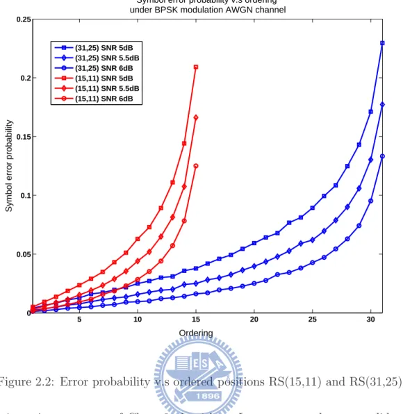
2.2 Error probability v.s ordered positions RS(15,11) and RS(31,25) . . . 7
2.3 Form of the parity check matrix suitable for iterative decoding by row operations . . . 10
3.1 BPSK mapping and the distribution of unreliable bits . . . 13
3.2 Candidates generation based on unreliable bits . . . 14
3.3 Gauss illustration . . . 17
3.4 Example of AG matrix . . . 17
3.5 Example of K-Best candidate selection, K=2 . . . 19
3.6 Example of parallel K-Best candidate selection with 4 layer for RS(15,11), T=1,. . .,4. . . 20
3.7 Example of subgroup selection in parallel K-Best scheme . . . 20
3.8 Example of subgroup in parallel K-Best scheme. . . 21
3.9 Example of path index and candidate sets for parallel K-Best algorithm . . 23
3.10 Example reduced index for parallel K-Best algorithm . . . 23
3.11 Example of chosen K candidate sets for parallel K-Best algorithm . . . 23
3.12 Parallel K-Best using constraint . . . 24
3.13 The chosen sets of parallel K-Best using constraint . . . 24
4.1 Performance comparison for K-Best of RS (15,11) BPSK mapping AWGN channel with different size of distance metric. . . 30
4.2 Performance comparison for K-Best of RS (15,11) BPSK mapping AWGN channel with different selection of K. . . 30
4.3 Performance comparison for parallel K-Best (K=300) of RS (15,11) BPSK mapping AWGN channel with different candidate number . . . 31 4.4 Performance comparison for parallel K-Best of RS (15,11) BPSK mapping
AWGN channel with constraint . . . 31 4.5 Performance of different soft decision decoding algorithm for RS (15,11)
BPSK mapping AWGN channel . . . 32 4.6 Performance for parallel K-Best of RS(31,25) BPSK mapping AWGN
chan-nel . . . 33 6.1 Illustration of sphere decoding algorithm . . . 44 6.2 Traditional K-Best algorithm . . . 44
List of Tables
3.1 Example of cost table . . . 15 3.2 Example of subgroup cost table . . . 21 4.1 Comparison between K-Best, parallel K-Best and parallel K-Best with
con-straint for RS (15,11). . . 34 4.2 Different candidate number of parallel K-Best algorithm for RS (15,11) . . 35 4.3 Computation comparison of ABP-ASD and proposed method . . . 35 4.4 Numerical comparison of ABP-ASD and proposed method for RS (15,11) . 35 4.5 Numerical comparison of ABP-ASD and proposed method for RS (31,25) . 36 4.6 Numerical complexity of proposed method of RS (15,11) . . . 36 4.7 Numerical complexity of proposed method of RS (31,25) . . . 36
Chapter 1
Introduction
1.1
Motivation
Reed-Solomon (RS) codes are one of the most widely used error correcting code for wireless communication and storage systems. The current issue about the RS code is to find an efficient way to improve the performance of traditional algebraic hard deci-sion Berlekamp-Messey(HD-BM) [1] algorithm. HD-BM algorithm does not use channel reliability information, this causes significant performance loss. Soft decision decoding algorithm takes advantage of the channel value, and is believed to have 2 ∼ 3 dB perfor-mance gain in additive white Gaussian noise (AWGN) channel. Guruswami and Vardy [2] have shown that Maximum-likelihood (ML) decoding of RS code is NP-hard. It remains an open area to find a soft decision code with moderate complexity with near ML perfor-mance.
Recently, the algebraic soft decision decoding (ASD) developed by Koetter and Vardy (KV) [3] use a list decoding technique outperforms Guruswami and Sudan (GS) [4] hard decision decoding method. On the other hand, Jiang and Narayanan (JN) [5] use adaptive parity check matrix and belief propagation to execute soft decision decoding based on iterative process. In [6], El-Khamy and McEliece combined JN and KV algorithm. They used belief propagation method to improve the reliability of the symbols and then fed these reliability information into a algebraic soft decision(KV) decoder.
There are several soft decision decoding algorithm based on the reliability-based de-coding. The order statistics decoding algorithm [7] sorts the received bits with respect
to their reliability, then the reprocessing step is designed to improve the hard decision codeword until a desired error performance is achieved. Other reliability-based decoding such as the generalized minimum distance (GMD) decoding algorithm [8], Chase algo-rithm [9] and a hybrid of chase and GMD algoalgo-rithms [10] use reliability information to enhance HD-BM algorithm. Sequential algorithm, or M-algorithm(K-Best) algorithm has been presented in [11], [12] offer a good deal in complexity reduction at the cost of some loss in performance. However, the previous paper only discuss the case for binary linear block codes or convolutional codes. Non-binary codes such as RS code is still open for sequential algorithm.
In this thesis, we develop a K-Best algorithm based on reliability-based scheme for soft RS decoding. Reliability-based decoding is based on reordering the received symbols according to their reliability measure. Hard decision reliability decoding use the k reliable symbols as information sequence and use the reordered generator matrix to re-encode the possible codeword. However, we did not do the re-encode process in this thesis. We summarize the decoding steps as follows:
1) For k reliable symbols, the possible candidates for each symbol are generated. We do not execute re-encoding process while use the property of the k reliable independent symbols to execute tree-oriented operation.
2) K-Best algorithm is introduced to collect the first k possible reliable symbols of K combination set. A proper constraint is also set up to reduce the computation complexity. 3) An erasure-only decoding is used to generate the rest of N-k unreliable symbols. 4) Combine k reliable symbols with N-k unreliable symbols as combination set. Each combination sets is calculated its distance metric between the received sequence. The one with minimum distance is regarded as the transmitted codeword.
1.2
Thesis organization
The rest of this thesis is organized as follows. Chapter 2 introduces the background of RS codes, and some soft decision decoding techniques. The proposed schemes, K-Best algorithm with constraint are presented in chapter 3. To accelerate the decoding speed, description for the parallel K-Best is in this section as well. The simulation results are
shown in chapter 4. The computation complexities of our K-Best algorithm are compared with popular algebraic soft decision decoding RS code is also in this chapter. Finally, a summary concluding our work is given in chapter 5. The techniques used in this thesis are all in chapter 6, including simplified cost function, re-encode decoding based on reliability ordering, sphere decoding and K-Best algorithm, and erasure-only decoding.
Chapter 2
Soft decoding of RS codes
Reed-Solomon(RS) codes were first introduced by Reed and Solomon in 1960 [13]. RS codes can be viewed as the symbol level cyclic non-binary BCH codes [14] whose symbols are in 𝐺𝐹 (2𝑞). The (N,k) RS code is with N symbols consisting of k messages
in 𝐺𝐹 (2𝑞). It is a maximum distance separable code with minimum distance of (N-k+1).
The decoding region is in 2𝑣 + 𝑒 < 𝑑𝑚𝑖𝑛, where 𝑒 is the number of erasures. The decoding
complexity is usually in the 𝑂(𝑁2). In this chapter, The system model of RS codes is
introduced in section 2.1. The RS code is then reviewed in section 2.2. For soft decision RS codes, symbol-level algebraic soft decision decoding such as GMD and Chase algorithm is described in section 2.3 and 2.4. Algebraic soft decision decoding algorithm(KV) is introduced in section 2.5. Iterative decoding of RS codes is shown in section 2.6.
2.1
System model of RS code
We use a systematic (N, k) Reed-Solomon(RS) code. The items in RS code are ele-ments of Galois Field 𝐺𝐹 (2𝑞) where 𝑁 = 2𝑞− 1. The operations in the process must be
operated over the Galois Field 𝐺𝐹 (2𝑞). Let B be the information sequence of length k.
The information sequence B multiply with RS generator matrix G to obtain the codeword sequence C of length N.
C = B × G (2.1)
Encode by G BPSK mapping Decoder AWGN channel Binary Extension
Figure 2.1: Channel model of RS code
Then c is BPSK modulated from the code symbols to the constellation symbols.
𝑥𝑗 = 𝑓 (𝑐𝑗) = (−1)𝑐𝑗, x = (𝑥0, 𝑥1, 𝑥2, . . ., 𝑥𝑁 𝑞−1) (2.2)
Then the modulated signal x is transmitted across the AWGN channel. The received sequences y = (𝑦0, 𝑦1, 𝑦2, . . . , 𝑦𝑁 𝑞−1) are soft values.
y = x + w (2.3)
Where w is the independent noise value Gaussian random variables with zero mean and variance 𝑁0/2. The system model of RS code is shown in Fig. 2.1.
2.2
Basic properties of Reed Solomon codes
The (N,k) RS code with bases 2 is defined over 𝐺𝐹 (2𝑞), where 𝑁 = 2𝑞 − 1. The
generator polynomial is used to encode the RS code. The generator polynomial g(x) of RS code which correct t or fewer error can be described by the minimum polynomials of 𝛼,𝛼2,𝛼3,. . .,and 𝛼2𝑡, and 𝛼 is a primitive element in 𝐺𝐹 (𝑞𝑚). Therefore the generator
polynomial has the following form
𝑔(𝑥) =
𝑖=2𝑡
∏
𝑖=1
(𝑥 − 𝛼𝑖) (2.4)
The generator polynomial has degree 2𝑡, thus an (N,k) RS code satisfies 𝑁 − 𝑘 = 2𝑡. Notice that g(x) can also be characterized by the minimum polynomials of 𝛼𝑏,𝛼𝑏+1,𝛼𝑏+2,. . .,and 𝛼𝑏+2𝑡−1 and can be generalized to
𝑔(𝑥) =
𝑖=𝑏+2𝑡−1
∏
𝑖=𝑏
(𝑥 − 𝛼𝑖) (2.5)
2.3
Generalized minimum distance algorithm
Generalized minimum distance (GMD) decoding is proposed by Forney [8]. The GMD decoding used reliability information of the received symbols to improve algebraic decod-ing. Based on successively erasing the least reliable symbols, GMD decoding runs the hard decision decoder. It is shown that GMD decoding can be asymptotically optimal. In ref [15] shows that an error-and-erasue method can correct all combinations of 𝑣 errors and 𝑒 erasures provided that 2𝑣 + 𝑒 ≤ 𝑑𝑚𝑖𝑛− 1. The GMD decoding consider all cases
of erasures 𝑒 ≤ 𝑑𝑚𝑖𝑛− 1 in the least reliable position(LRPs) which are the most likely
positions to be in error. The decoding method are as follows:
1. GMD decoding generates the hard decision Z from the received sequence y and assigns a reliability value to each symbol Z.
2. GMD decoding generates a list of ⌊𝑑𝑚𝑖𝑛+1
2 ⌋ sequence by modifying the hard decision
sequence Z with erasing the least reliable symbols.
3. GMD decoding decodes each modified Z into a codeword. Then it feeds Z into an algebraic decoder.
4. GMD decoding computes the distance metric of each generated symbol and selects the one with the minimum distance metric as the solution.
2.4
Chase decoding algorithm
Chase algorithm [9] is the generalization of the GMD algorithm. Chase-1 algorithm does not consider reliable or unreliable positions. It always generates 𝐶𝑛
𝑑𝑚𝑖𝑛 2
candidate codewords by considering all possible combinations of ⌊𝑑𝑚𝑖𝑛
2 ⌋ in the hard received sequence
Z. But the computational complexity of Chase-1 algorithm is too heavy, few people discuss the algorithm.
Chase-3 algorithm does similar operations as the GMD algorithm, except the erasure operation in the GMD is being replaced by flipping the least reliable symbols. For binary codes, Chase-3 algorithm achieves the same error performance as GMD and require same computational complexity.
decod-5 10 15 20 25 30 0 0.05 0.1 0.15 0.2 0.25
Symbol error probability v.s ordering under BPSK modulation AWGN channel
Ordering
Symbol error probability
(31,25) SNR 5dB (31,25) SNR 5.5dB (31,25) SNR 6dB (15,11) SNR 5dB (15,11) SNR 5.5dB (15,11) SNR 6dB
Figure 2.2: Error probability v.s ordered positions RS(15,11) and RS(31,25) ing. It is an improvement of Chase-3 algorithm. It generates a larger candidate lists. All possible errors in the range of ⌊𝑑𝑚𝑖𝑛
2 ⌋ of LRPs is used to improve Z. The algorithm
exhaustively flip the least reliable symbols and run the hard decision decoder. The candi-date list grows exponentially with 𝑑𝑚𝑖𝑛. Since the larger candidate list leads to a greater
possibility to correct the errors. Chase-2 algorithm performs a much better performance than Chase-3 algorithm.
Among three algorithm, Chase-2 algorithm is the best algorithm considering the trade-off between complexity and performance.
Fig. 2.2 shows the error probability versus reliability ordering for RS(15,11) and RS(31,25). From the figure, we can observe that the error probability has an exponential like curve. The received vectors are sorted according to their reliabilitiew. The first k positions can be regarded as reliable positions, and the last N-k positions are unreliable positions. The least reliable N-k region has the higher probability to occur errors than
the previous k positions. This tells why the GMD decoding and Chase algorithm work. They generate the candidate codewords by dealing with the last N-k positions, and feed the modified candidate codewords in to hard decision decoder. They hope that the hard decision decoder can help them correct the errors occurred in the previous k position, if exists. However, the drawback of these two algorithm is that if the error does not occur in the last N-k region, and all concentrated in the reliable k regions and the number of errors are larger than the error correction capabilities. Then, the decoder will never find a correct codeword.
2.5
Algebraic soft decision decoding algorithm
Guruswami and Sudan (GS) invented a polynomial-list decoding algorithm [4] for RS codes capable of correcting beyond half the minimum distance of the code. Koetter and Vardy developed an algebraic soft decision(ASD) decoding [3] based on GS algo-rithm using the reliability information to assign multiplicity for RS codes. the decoding scheme is briefly summarized as follows: The transmitted codeword can be described as (𝑓 (𝛼1), 𝑓 (𝛼2), . . . , 𝑓 (𝛼𝑁)) the received vector is (𝛽1, 𝛽2, . . . , 𝛽𝑁). The basic idea is to find
a 𝑓 (𝑥) which fits as many points in (𝑓 (𝛼𝑖), 𝛽𝑖) pairs. The KV algorithm consists of two
main steps, interpolation step and factorization step.
Step 1) Interpolation: Construct a bivariate polynomial 𝑄(𝑥, 𝑦) of minimum (1,k-1) de-gree, which has a zero order of 𝑣 at (𝛼𝑙, 𝛽𝑙), l=1,. . .,N, i.e: if 𝑄(𝑥 − 𝛼𝑙, 𝑦 − 𝛽𝑙) involves no
term of degree less than 𝑖 + 𝑗 = 𝑣.
Step 2) Factorization: Generate a list of y-roots,i.e: 𝐿 = 𝑓 (𝑥) ∈ 𝐹 [𝑥] : (𝑦 − 𝑓 (𝑥)∣𝑄(𝑥, 𝑦), 𝑑𝑒𝑔(𝑓 (𝑥)) < 𝑘)
Then, pick up the most likely codeword 𝑓 (𝑥) from the list 𝐿.ˆ
The ultimate gain of algebraic soft decoding (ASD) over AWGN channel is about 1dB. The complexity is scalable but prohibitively large for huge multiplicity.
2.6
Iterative Reed-Solomon decoding algorithm
In [5], Jiang proposed the iterative decoding algorithm based on sum-product algo-rithm(SPA). The main idea is to adapt the parity-check matrix at each iteration according
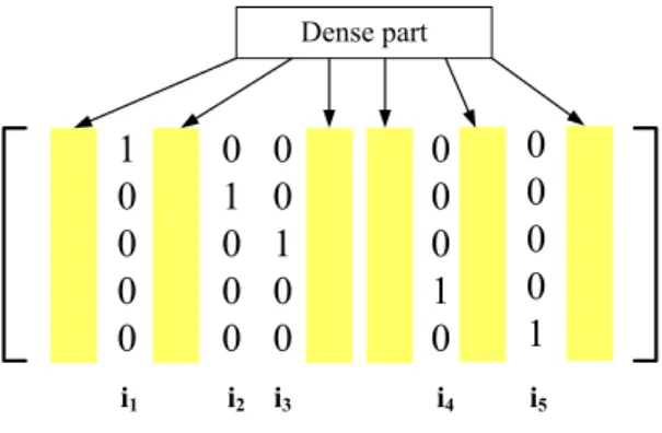
to the reliabilities such that the unreliable bits correspond to a sparse matrix, so that the SPA algorithm can continue applying to the adapted parity check matrix. The adapta-tion prevents iterative decoding from getting stuck at local equilibrium region, thus, the decoding process can continue to a convergence region. The following is the parity-check matrix of an (N,k) RS code over 𝐺𝐹 (2𝑞):
𝐻𝑠= ⎛ ⎜ ⎜ ⎜ ⎜ ⎜ ⎜ ⎝ 1 𝛽 . . . 𝛽(𝑁 −1) 1 𝛽2 . . . 𝛽2(𝑁 −1) . . . 1 𝛽(𝑑𝑚𝑖𝑛−1) . . . 𝛽(𝑑𝑚𝑖𝑛−1)(𝑁 −1) ⎞ ⎟ ⎟ ⎟ ⎟ ⎟ ⎟ ⎠ (2.6)
where 𝛽 is a primitive element in 𝐺𝐹 (2𝑞), 𝑑
𝑚𝑖𝑛 = 𝑁 − 𝑘 + 1. Let 𝑛 = 𝑁 × 𝑞 and
k = 𝑘 × 𝑞 be the length of the codeword and information at the bit level, respectively. 𝐻𝑠 has an equivalent binary image expansion 𝐻𝑏 (One can find in [15]), where 𝐻𝑏 is an
(𝑛 − k) × 𝑛 binary parity-check matrix.
The iterative algorithm is composed of two stages: 1) The matrix updating stage.
2) The bit-reliability updating stage.
Assume c = (𝑐0, 𝑐1, 𝑐2, . . . , 𝑐𝑁 𝑞−1) is the binary representation of RS codeword. By
us-ing BPSK modulation and transmitted the codeword over an AWGN channel the received vectors y = (𝑦0, 𝑦1, 𝑦2, . . . , 𝑦𝑁 𝑞−1) can be given by
y = c + w (2.7)
where w is the AWGN noise. The initial reliability of each bit can be expressed in terms of the log-likelihood ratios(LLR):
𝐿(0)(𝑐𝑖) = 𝑙𝑜𝑔
𝑃 (𝑐𝑖 = 0∣𝑦𝑖)
𝑃 (𝑐𝑖 = 1∣𝑦𝑖)
(2.8) where 𝑐𝑖 stands for codeword and 𝑦𝑖 stands for received vector in the bit
represen-tation. The magnitude of the received LLRs ∣𝐿(𝑐𝑖)∣ are sorted in an descending order
𝑖𝑁,. . . , 𝑖𝑁 −𝑘,. . . , 𝑖2, 𝑖1, the bit 𝑐𝑖𝑁 is the most reliable and the bit 𝑐𝑖1 is the least reliable.
The algorithm begins with the original parity-check matrix 𝐻𝑏, and reduce the 𝑖1 th
col-umn of 𝐻𝑏 to a form [10 . . . 0]𝑇. the process is continued to reduce (𝑁 − k)-th columns of
Dense part
i1 i2 i3 i4 i5
Figure 2.3: Form of the parity check matrix suitable for iterative decoding by row opera-tions
In the matrix updating stage. For the 𝑣-th iteration, the vector of LLRs will be 𝐿𝑣 = [𝐿(𝑣)(𝑐
1), 𝐿(𝑣)(𝑐2), . . . , 𝐿(𝑣)(𝑐𝑛)] (2.9)
and 𝐿0 is determined from the channel output. Then, the parity-check matrix is
reduced to a form based on 𝐿𝑣
𝐻𝑏𝑣 = 𝜙(𝐻𝑏, ∣𝐿𝑣∣) (2.10)
In the bit-reliability updating stage, the extrinsic LLR vector 𝐿𝑣
𝑒𝑥𝑡 is generated by 𝐿𝑣
using the SPA based on the previous adapted parity-check matrix 𝐻𝑣 𝑏
𝐿(𝑣)𝑒𝑥𝑡= 𝜓(𝐻𝑏𝑣, 𝐿𝑣) (2.11)
For each bit, the extrinsic LLR is updated according to 𝐿(𝑣)𝑒𝑥𝑡(𝑐𝑖) = 𝑛−𝑘 ∑ 𝑗=1,𝐻𝑣 𝑗𝑖=1 2𝑡𝑎𝑛ℎ−1 ⎛ ⎝ 𝑛 ∏ 𝑝=1,𝑝∕=𝑖,𝐻𝑣 𝑗𝑝=1 𝑡𝑎𝑛ℎ(𝐿 (𝑣)(𝑐 𝑝) 2 ⎞ ⎠ (2.12)
The bit-reliability is then updated as
𝐿(𝑣+1) = 𝐿(𝑣) + 𝛼𝐿(𝑣)𝑒𝑥𝑡 (2.13)
where 0 ≤ 𝛼 ≤ 1 is a damping coefficient. Then, take hard decision of the decoded bit codeword ˆ𝑐𝑖 ˆ 𝑐𝑖 = ⎧ ⎨ ⎩ 0, 𝐿(𝑣+1)(𝑐 𝑖) > 0 1, 𝐿(𝑣+1)(𝑐 𝑖) < 0 (2.14) The termination criterion is, if all the checks are satisfied, output the estimated bits; else if 𝑣 = 𝑣𝑚𝑎𝑥 iteration, declare a decoding failure; otherwise set v to v+1 and go for
The drawback of the iterative decoding by adapting parity-check matrix of RS code is that the algorithm has the ”error floor” problem. And the iterative decoding needs different iteration to complete the decoding process.
Chapter 3
Proposed soft RS decoding with
K-Best algorithm
Reliability based decoding with ordered statistics [7] has been shown to be efficient to decode binary linear block codes. In this chapter, based on reliability decoding and re-encode process we introduce a new matrix AG for our decoding operation. We didn’t do the re-encode process as the previous paper. The candidate of each reliable symbols is generated when the received soft value is determined. We take advantage of the more reliable column of matrix AG, then transform it into a tree-oriented problem. The K-Best algorithm is introduced to search the possible candidate previously generated. Since the decoding speed is the drawback of the K-Best algorithm, parallel K-Best algorithm is used to improve the speed issue. The K-Best algorithm with constraint is used to reduce the computation complexity, especially the comparison for the parallel K-Best algorithm. Erasure-only decoding is described next to use the property of RS codes, we can regard the N-k unreliable position as erasures. The k-reliable symbols of K-Best combinational sets can be used to decode the other N-k erasures. A brief summary is at the end of this chapter, to describe the decoding flow of the proposed soft RS decoding algorithm.
∗Note: The method including cost function, re-encode, sphere decoding, K-Best algorithm and erasure-only decoding in this chapter can be found in chapter 6, appendix.
1
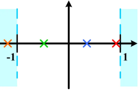
-1
Figure 3.1: BPSK mapping and the distribution of unreliable bits
3.1
Pre-processing
In Pre-processing, we first generate the symbol candidates, and reorder the symbol based on reliability. The generator matrix is also permuted according to the reliability. Then, Gauss elimination is used to avoid the correlation between reliable symbols. At last, re-encode is used to generate the possible codeword sets. It is observed in the pre-processing process that reliable symbols do not need to execute Gauss elimination, since they are already independent.
3.1.1
Candidate generation
Decoding based on most reliable independent position (MRIP) requires the ordering of the received sequence according to their reliability. At first, we use hard decision symbols to be the foundation to choose the reliable symbols and produce the candidates. After DE-BPSK, we declare the hard decision of y as z, where z = (𝑧0, 𝑧1, 𝑧2, . . . , 𝑧𝑁 𝑞−1).
The vector z is transmitted from the binary sequence into symbol sequence Z where Z = (𝑍0, 𝑍 − 1, . . . , 𝑍𝑁 −1). Every symbol 𝑍𝑗 where 𝑗 is form 0 to 𝑁 − 1 is composed by
(𝑧𝑗𝑞, 𝑧𝑗𝑞+1, . . . , 𝑧𝑗𝑞+(𝑞−1)).
Based on the re-encoding schemes, the selection of candidate is as follows. We decide the unreliable bits number of symbols and generate the candidates correspond to those symbols. Because those bits are not reliable, we consider all possible combination of their position with 1 and 0.
Fig. 3.1 shows the example of unreliable bits. We can set up criterion to decide how many number of unreliable bits need to be considered. The criterion is as follows:
Unreliable bits
generate
Figure 3.2: Candidates generation based on unreliable bits Design criterion
1) The received soft values lie between 1 and −1.
2) The number of unreliable bits could be decided off-line according to the absolute soft values.
After the unreliable bits are found, DE-BPSK is done in the next. According to Fig. 3.1, the corresponding hard decision bits of 𝑗th symbol (𝑧0,𝑗, 𝑧1,𝑗, 𝑧2,𝑗, 𝑧3,𝑗) are (1, 0, 0, 1).
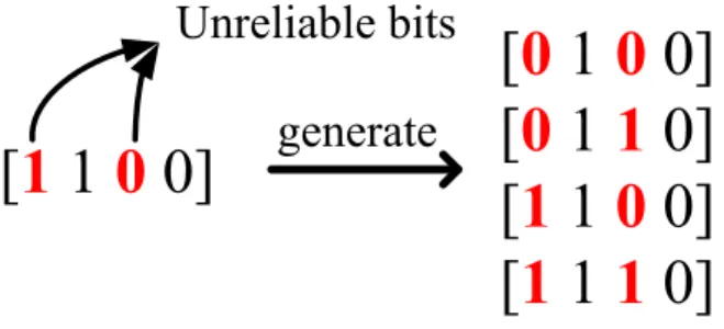
Then, for each symbol we could use the unreliable bits to produce its candidates. Fig. 3.2 shows the example of candidate generation.
To produce all candidates of the symbol, there are three steps as follows.
1) We decide the unreliable bits number of the symbol and mark the position of these unreliable bits.
2) We use 1 and 0 to produce 2𝑣 combination sets, where 𝑣 is the number of unreliable
bits.
3) There are 2𝑣 sets of 𝑣 unreliable bits, they would be placed into the marked position
of unreliable bits.
After the above three steps, all candidates would be generated. We use the above three steps and continue to demonstrate the previous example. There are two unreliable bits, 𝑧0,𝑗 and 𝑧2,𝑗, corresponding to 𝑦0,𝑗 and 𝑦2,𝑗. The positions of these bits are 0 and 2.
Then, all 22 combination sets of 1 and 0 are generated. They are (0, 0), (0, 1), (1, 0) and
(1, 1). Next, we replace the origin hard decision symbol bits position with these bit sets. The origin hard decision bits of the symbol are (1, 0, 0, 1). Therefore, the candidates are (0, 0, 0, 1), (0, 0, 1, 1), (1, 0, 0, 1) and (1, 0, 1, 1).
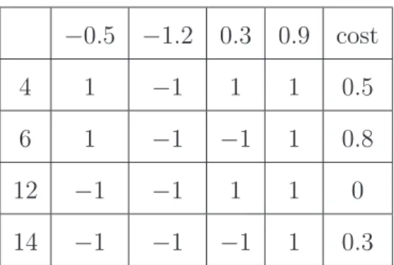
Table 3.1: Example of cost table −0.5 −1.2 0.3 0.9 cost 4 1 −1 1 1 0.5 6 1 −1 −1 1 0.8 12 −1 −1 1 1 0 14 −1 −1 −1 1 0.3
the example of different cost between candidates and received soft values. We order the candidates of the symbol by their cost compared to the received value. Every symbol 𝑍𝑗
would have its own candidates ( ˆ𝑍𝑗,0, ˆ𝑍𝑗,1, . . . , ˆ𝑍𝑗,𝑚). The selection of 𝑚 which is between 1
to 𝑁 +1 is obtained by the number of unreliable bits. The candidates of 𝑗th symbol can be denoted as a vector ˆ𝑍𝑗. We calculate the cost between candidates ˆ𝑍𝑗,𝑖and the received soft
values 𝑦, then arrange ˆ𝑍𝑗,𝑖in a ascending order denoted as 𝑆𝑗 = (𝑆𝑗,0, 𝑆𝑗,1, . . . , 𝑆𝑗,𝑚).Where
the permutation is denoted as 𝜆1.
𝑆𝑗 = 𝜆1( ˆ𝑍𝑗) (3.1)
Obviously, 𝑆𝑗,0is the hard decision symbol. The candidate with the smallest cost value
is the most possible transmission symbol. First 𝑘 reliable candidate sets are used in this algorithm through the process, and the last 𝑁 − 𝑘 candidate sets would be used in the erasure only decoding.
After producing the candidates of all symbols, we compose all possible candidate sets. Fixed number (𝑚) of candidate symbols is used in re-encode method. There are 𝑚𝑘
possible combination sets to operate re-encode process. These possible candidate sets should execute the same operation as the columns of 𝐺.
3.1.2
Reliability ordering
For each hard decision symbol 𝑆𝑗,0, reliability is calculated by adding the corresponding
absolute value of received soft values 𝑦𝑗.
R𝑗 = Σ𝑞−1𝑖=0 ∥𝑦𝑗𝑞+𝑖∥ (3.2)
Then S is rearranged to be S′ = (𝑆′
0, 𝑆1′, 𝑆2′, . . . , 𝑆𝑁 −1′ ).
The symbols are re-arranged as S′. We denote the permutation as 𝜆
2. We selected
first k most reliable symbols (𝑆′
0, 𝑆1′, . . . , 𝑆𝑘−1′ ) to perform the pre-processing. Since the
columns of G correspond to the position of symbols, thus we permute the columns of generator matrix based on the ordering of reliability. After the permutation of generator matrix G, the new matrix can be marked as G′.
𝑆′ = 𝜆
2(𝑆) (3.3)
𝐺′ = 𝜆2(𝐺) (3.4)
3.1.3
Re-order generator matrix
The first 𝑘 columns of 𝐺′ are not necessarily independent while in re-encoding scheme,
thus such 𝑘 columns can not represent the information set. We are going to rearrange the first 𝑘 columns of G′ to make each 𝑘 column independent. The rearranged matrix is G′′
and its first 𝑘 columns are linearly independent. After the rearrange operation 𝜆3, the
columns of G′′ also maintain the descending order of the reliability values. The operation
𝜆3 could be regarded as Gaussian eliminations which let G′′ in the reduce echelon form
that contain only one 1. We use matrix A to represent the Gaussian elimination operation.
G′′= 𝜆
3(G′) = G′ × A (3.5)
The generator matrix becomes G′′ after the Gaussian elimination which is shown
as Fig. 3.3. The corresponding symbols should execute the same operation, then the resultant is denoted as S′′.
S′′ = 𝜆
3(S′) = S′ × A (3.6)
Every possible set of S′′ should do the same operations to produce the possible
code-word in re-encode process. Because the G′′ is systematic matrix, it means the
corre-sponding S′′ is the possible independent message sets. The possible message sets multiply
generator matrix G to produce possible codeword sets. In re-encode method, we calculate the cost between the received soft value and possible codeword and decide the codeword with minimum cost as the decoded codeword.
k k
I
×''
G
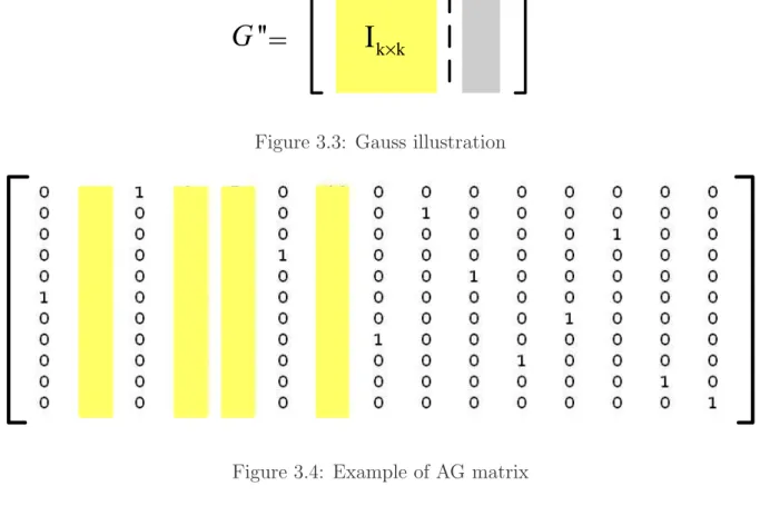
Figure 3.3: Gauss illustration
Figure 3.4: Example of AG matrix
3.1.4
Re-encoding process
In re-encode method, every S′ set must multiply matrix A and then multiply matrix
G. Because there are 𝑚𝑘 sets, re-encode method needs a lot of multiply operations. We
want to reduce the operation number, so we multiply A and G together to be matrix AG. Fig. 3.4 shows an example of the matrix AG. Then every S′ set only needs to multiply
matrix AG once. The re-encode process speeds up 1.5 times. It reduces the operation number and produces the same codeword sets.
After we produce matrix AG, we discover that there is a special property of matrix AG. The property of matrix AG can be divided in to two parts. First, the columns with only one 1 correspond to the position of reliable symbols can be regarded as the permu-tation of 𝑘 × 𝑘 identity matrix. Second, the columns correspond to the position of 𝑁 − 𝑘 unreliable symbols can be regarded as the combination of the other 𝑘 reliable symbols. Observing the matrix AG, we find out that the 𝑘 reliable symbols are independent. 1) We marked the position of 1 in the columns of matrix AG which has only one 1 as index L. L = (𝑙0, 𝑙1, 𝑙2, . . . , 𝑙𝑘−1) are indexes corresponding to the most 𝑘 reliable symbols.
be selected in K-Best scheme.
3) The order of 𝑘 column with only one 1 stands for the position of the corresponding reliable symbol.
4) The value of index 𝑙𝑖(𝑖 = 0 ∼ 𝑘 − 1) represents for the 𝑙𝑖th transmitted symbol.
The index would point out the most 𝑘 reliable symbol corresponding to the 𝑙𝑗th symbol
of the received codeword, respectively.
3.2
Candidate selecting
In section 3.1.4, it has mentioned that the possible candidate sets will be 𝑚𝑘. This is
a large number when k increases, and it is not feasible to use these candidate sets to do the re-encoding process. In the following section, we proposed K-Best algorithm, parallel K-Best algorithm and parallel K-Best algorithm with constraint to reduce the number of candidate sets.
3.2.1
K-Best algorithm
There are 𝑚𝑘 combination sets of S′ needed to multiply matrix AG, which still leads
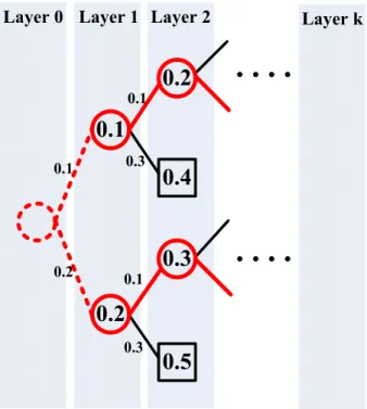
to a large number of operations. The independent property of matrix AG can be used to reduce the re-encode operation. Thus, we can use the independent property of matrix 𝐴𝐺 to execute 𝐾-Best operation. 𝐾-Best operation needs 𝑘 layers to select the candidate sets. Every candidate set of symbol would be a layer in 𝐾-Best. A tree Fig. 3.5 is used to represent the whole process.
We assume an origin point in layer 0 and use the dotted line to mark it as a pseudo node. A pseudo node is set up to start the tree-like algorithm. The path between layer 0 and layer 1 would be marked as dotted line too. Then, the first candidate sets would spread up at layer 1. In the Fig. 3.5, the node represents the accumulated cost. There are 𝑚 candidates of 𝑗th symbol in each layer where S′
𝑗 = (𝑆𝑗,0′ , 𝑆𝑗,1′ , . . . , 𝑆𝑗,𝑚′ ).
The value in the line stands for the cost of that candidate compared to the received soft value. The value of node stands for the accumulated cost. Each layer accumulates the cost from the previous layer, and then chooses the combination sets of K minimum
0.1 0.1
Layer 0 Layer 1 Layer 2
0.2
0.3
0.1
0.2
0.3 0.3 Layer k0.4
0.5
0.1 0.2Figure 3.5: Example of K-Best candidate selection, K=2
cost candidates. The chosen path and node would be marked as line and circle in solid line. The next layer would start from the chosen node. The stop criterion is that the candidates of 𝑘 reliable symbols are all considered.
We can summary the process in four steps as follows until the stop criterion is achieved. 1) For each parent node, it spreads out the possible candidates as child node in that layer 2) Each child node accumulates the cost
3) We choose K minimum cost sets in the decoding layer.
4) Check the stopping criterion. If the stopping criterion is not achieved, start the next layer from chosen K nodes in last layer
Therefore, we have less candidate sets chosen by K-Best method than the re-encode method.
3.2.2
Parallel K-Best algorithm
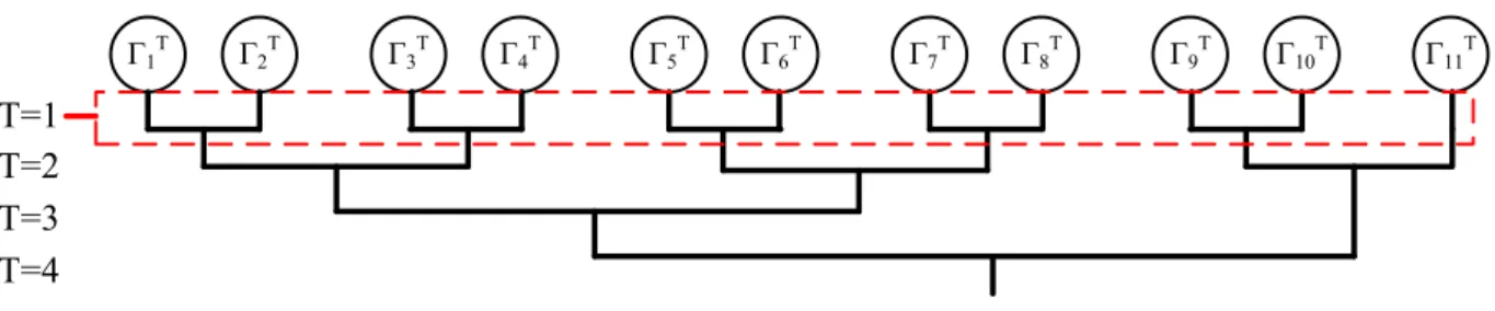
Although the K-Best method reduces the operation, the speed of execution is still not good enough. In this thesis a parallel K- Best algorithm is proposed to improve the speed issue, it separates most 𝑘 reliable candidate sets into several groups. There are 𝑞 layers in Galois Field 𝐺𝐹 (2𝑞). Fig. 3.6 shows an example of RS(15,11) with 4 layers.
Γ1 T Γ2 T Γ3 T Γ4 T Γ5 T Γ6 T Γ7 T Γ8 T Γ9 T Γ10 T Γ11 T T=1 T=2 T=3 T=4
Figure 3.6: Example of parallel K-Best candidate selection with 4 layer for RS(15,11), T=1,. . .,4. Γ1 T Γ2 T Γ3 T Γ4 T Γ5 T Γ6 T Γ7 T Γ8 T Γ9 T Γ10 T Γ11 T T=1 T=2 T=3 T=4 1 1 1 1 1 2
Figure 3.7: Example of subgroup selection in parallel K-Best scheme Here are the steps for parallel K-Best algorithm.
1) For the selection of the candidate, we define some parameters as following. Here, 𝑇 stands for the number of layer from 1 to 𝑞, 𝛼1 is the number of sub-groups with two
candidate sets in that layer and 𝛼2 is the number that a sub-group has only one candidate
sets in that layer. 𝛼1 and 𝛼2 are integers, and 𝛼2 would always be 0 or 1. Fig. 3.7 is
the example of subgroup selection in parallel K-Best scheme. In an (𝑁, 𝑘) RS code, 𝛼1
would be initialized as 𝑘/2 and 𝛼2 would be initialized as 𝑘%2 at first layer. % stands for
module.
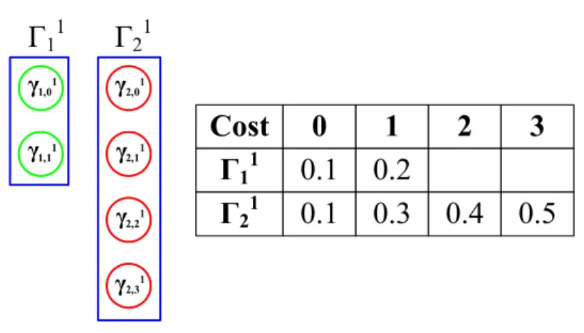
2) We use a sequential tree-like method to help us choose candidate sets in 𝐾-Best scheme. If there are two input candidate sets (ΓT
1, ΓT2) with (𝑚𝑇1, 𝑚𝑇2) candidates in layer
𝑇 where ΓT 1 = (𝛾1,0𝑇 , 𝛾1,1𝑇 , . . . , 𝛾1,𝑚𝑇 1−1) and Γ T 2 = (𝛾2,0𝑇 , 𝛾2,1𝑇 , . . . , 𝛾2,𝑚𝑇 2−1), and 𝛾 𝑇 𝑗,𝑖 means the
𝑖-th candidate of input candidate set ΓT
j in layer 𝑇 . There are total 𝑀𝑇 = 𝑚𝑇1 × 𝑚𝑇2
combinational candidate sets. Fig. 3.8 shows an example of the subgroup. We must use 𝐾-Best method to choose 𝐾 combined candidate sets with smaller cost value. As we choosing these candidate sets, we must denote the cost value and the index of each candidate combination sets. The index here means that the candidates of combined sets which its original position is in input candidate set?
γ1,01 γ2,01 γ1,11 γ2,11 γ2,21 γ2,3 1
Cost
0
1
2
3
Γ
110.1
0.2
Γ
210.1
0.3
0.4
0.5
Γ
11Γ
21Figure 3.8: Example of subgroup in parallel K-Best scheme.
Table 3.2: Example of subgroup cost table Accumulated Cost order of Γ1
1 order of Γ12 0.2 0 0 0.3 1 0 0.4 0 1 0.5 0 2 0.5 1 2 0.6 0 3 0.6 1 2 0.7 1 3
Obviously, each input candidates sets needs 𝑀𝑇 indexes. The cost information is
saved in another 𝑀𝑇 register. Thus, total 3𝑀𝑇 registers are needed to be saved for
𝐾-Best scheme. Table. 3.2 shows an example of 3𝑀𝑇 registers to save the index and cost
information.
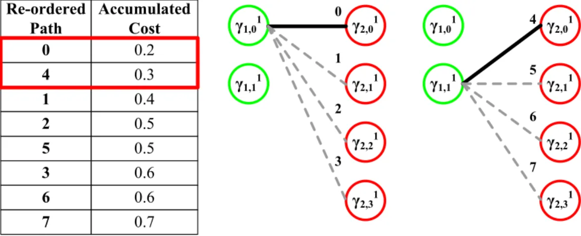
Now we use a scheme which needs only 2𝑀 register to execute 𝐾-Best algorithm. 1) We produce the combination candidate sets in sequence as following. We fix the candidate of ΓT
1 and displace the candidates in ΓT2 until all 𝑚𝑇2 candidates are changed.
Then we move on to the next candidate of ΓT
1, and do the same process as above. Fig.
3.9 shows an example of producing path index and candidate sets for parallel K-Best algorithm.
2) During producing the combinational candidate sets, we give every combination set an index number Ω from 0 to 𝑀𝑇 − 1 sequentially, and denote the accumulated cost of every
combined candidate sets.
3) As all 𝑀𝑇 combination candidate sets are produced, all combination sets are sorted
by the cost and also the index is permuted according the new order.
4) 𝐾-Best scheme choose 𝐾 candidate combination sets which are the input sets of next layer. The elements of chosen combination sets are traced by the index Ω. The element from ΓT
1 is the 𝛾1𝑇 th term of the input candidate set where 𝛾1𝑇 = Ω/𝑚𝑇2. The element
from ΓT
2 is the 𝛾2𝑇 th term of the input candidate set where 𝛾2𝑇 = Ω%𝑚𝑇2. Then we could
use only 𝑀 registers to memorize the index of elements in combination sets. Fig. 3.10 shows an example of reduced index for parallel K-Best algorithm
5) Then, 𝐾-Best scheme is executed in every sub-group independently.
6) After the 𝐾-best algorithm, every sub-group chooses its own candidate sets. Fig. 3.11 shows the chosen candidate sets for parallel K-Best algorithm.
7) We repeat the steps above until the output candidate sets have 𝑘 elements.
3.2.3
Parallel K-Best algorithm with constraint
Parallel K-Best method reduces the total comparing number for selecting the candidate sets. As the 𝑘 becomes bigger, we need a large number of sorting. To prevent the sorting complexity becomes too heavy, we decide to use a bound to consistent the number of sorting.
γ1,01 γ2,01 γ1,11 γ2,11 γ2,21 γ2,31 0 1 2 3 γ1,01 γ2,01 γ1,11 γ2,11 γ2,21 γ2,31 4 5 6 7 Path Accumulated Cost 4 0.3 0 0.2 5 0.5 1 0.4 6 0.6 2 0.5 7 0.7 3 0.6
Figure 3.9: Example of path index and candidate sets for parallel K-Best algorithm
γ1,01 γ2,01 γ1,11 γ2,11 γ2,21 γ2,31 0 1 2 3 γ1,01 γ2,01 γ1,11 γ2,11 γ2,21 γ2,31 4 5 6 7 Re-ordered Path Accumulated Cost 5 0.5 0 0.2 3 0.6 4 0.3 6 0.6 1 0.4 7 0.7 2 0.5
Figure 3.10: Example reduced index for parallel K-Best algorithm
γ1,01 γ2,01 γ1,11 γ2,11 γ2,21 γ2,31 0 1 2 3 γ1,01 γ2,01 γ1,11 γ2,11 γ2,21 γ2,31 4 5 6 7 Re-ordered Path Accumulated Cost 5 0.5 0 0.2 3 0.6 4 0.3 6 0.6 1 0.4 7 0.7 2 0.5
γ1,01 γ2,01 γ1,11 γ2,11 γ2,21 γ2,31 0 1 2 3 γ1,01 γ2,01 γ1,11 γ2,11 γ2,21 γ2,31 4 5 6 7 Bound = 0.6 Path Accumulated Cost 4 0.3 0 0.2 5 0.5 1 0.4 6 0.6 2 0.5 7 0.7 3 0.6
Figure 3.12: Parallel K-Best using constraint
γ1,01 γ2,01 γ1,11 γ2,11 γ2,21 γ2,31 0 1 2 3 γ1,01 γ2,01 γ1,11 γ2,11 γ2,21 γ2,31 4 5 6 7 Bound = 0.6 Path Accumulated Cost 2 0.5 0 0.2 5 0.5 4 0.3 1 0.4
Figure 3.13: The chosen sets of parallel K-Best using constraint
In the process of parallel K-Best method, we define different bound for each layer. The bound of each layer is defined by observing the cost distribution. The accumulated cost of candidate sets smaller than the bound are chosen. The chosen combination sets would be re-arranged according the order of cost.
In the Fig. 3.12, the bound is defined as 0.6, and K is set to equal 2. Thus, the combination sets 0, 1, 2, 4 and 5 marked as black dotted line in order which would be chosen to be the possible K candidates.
By using the constraint and combined with the K-Best algorithm, the number of sorting sets are decreased. Fig. 3.13 shows the example of constraint, in this example There are total five candidates fall in the bound. If K is equal to 2, then the path 0 and path 4 are the selected combinational sets. The complexity of operation is reduced and the speed of process is faster almost two times than before.
3.3
Erasure-only decoding
We use K-Best method to choose K minimum cost sets correspond to K minimum candidate sets. Every possible unreliable sets and the chosen K-Best sets are combined together as possible codeword sets. Since re-encode process needs to deal with the order-ing of generator matrix. In C program, this means the process needs a lot of temporary memory to store related data. Besides, the criterion for selecting codeword is only based on K-Best cost, it is not sufficient to obtain good performance. From AG matrix, we notice that the unreliable symbols can be composed by the reliable symbols. Thus, the erasure-only decoding is suitable for this task. And it adds another condition to see whether the codeword is in the generated candidate sets. Based on the above improve-ment of the decoding process, the re-encode process is replaced by erasure only decoding. Every possible codeword are put into syndrome equation to find out whether the possible codeword is in the codeword set of this system. If the syndrome equations are all zeros, it means that the possible codeword is in the codeword set. We choose the codeword under the following constraint
(1) Syndrome equations are all zeros
(2) The codeword with the minimum accumulated cost.
The codeword with the above two condition should be the transmission codeword. The method mentioned before this section needs S′′ multiply matrix AG to obtain
possible codeword sets. There are just one constraint, to find minimum cost. The possible codeword set is judged by which codeword set has minimum cost. In this section, we do not execute re-encode method because we do not use S′ to multiply matrix AG. Here, we
add another constraint to consider the possible codeword. Is it in the codeword sets or not? This will help us choosing the right possible codeword. Using the minimum cost and syndrome equation constraints make us reach better performance then re-encode. But we discover that there are three kinds of errors as follows.
1) The transmitted codeword is in the K-Best sets, but the syndrome equations of it (the transmitted set) are not all zeros. This kind of error is produced because the candidates of unreliable symbols are not chosen properly. We could choose more unreliable bits to extend the possible candidates of unreliable symbols.
transmitted codeword is larger than the Kth Best sets, the transmitted codeword is not chosen. We could solve this error by choosing the larger K to contain the transmitted codeword.
3) The transmission codeword is in the K-Best sets and the syndrome equations are all zeros but we do not choose the transmitted set. The reason is that there is another possible codeword set which cost is smaller than the transmitted set and the syndrome equations are all zero, too. Under these conditions, we choose the wrong codeword which satisfy both constraints better than the transmitted one. This kind of error is the maximum-likelihood error, since the noise interference caused the right answer jump to another, thus we could not solve this problem
Though we use constraint for accumulated cost and syndrome equation to improve the performance, there still needs a better algorithm. We realize that the accumulated cost of MRIP 𝑘 symbols being calculated by K-Best should be replaced by cost of all 𝑁 candidates. Because the codeword sets produced by syndrome equation are possible transmitted codeword, the most possible codeword set should consider the cost of all 𝑁 symbols. After we change the constraint with the cost of 𝑁 symbols, the performance is improved.
3.4
Summary
The proposed algorithm consists of three parts, pre-processing, candidate selecting and erasure only decoding. It should be mentioned that in pre-processing process, the matrix AG shows that after reliability ordering from the received value, the most k reliable symbols are already independent. It implies we can choose the candidate sets after the symbols being reordered by reliability. Thus, it is needless to do any operation for gen-erator matrix. For candidate selecting, the K-Best algorithm is introduced to reduce the computation complexity for possible candidate sets. Since the decoding speed is too slow for the layer by layer property of the K-Best algorithm, the parallel K-Best algorithm is introduced. The parallel K-Best algorithm divides the candidates sets into several groups, each subgroup chooses local K-Best candidate. The decoding process is continued until the candidate sets is combined with 𝑘 symbols. The parallel K-Best algorithm reduces
the computation layer from k to q, thus increases the decoding speed and decrease the computation complexity. Finally, the re-encoding process is replaced by the erasure-only decoding.
Chapter 4
Simulation results and complexity
comparison
In this section, RS(15,11) and RS(31,25) are simulated for comparing the proposed gorithm and the other RS code such as hard decision Berlekamp-Massy algorithm, KV al-gorithm, adaptive belief propagation algorithm(JN), adaptive belief propagation-algebraic soft decoding(ABP-ASD), and sphere decoding algorithm. The signal is modulated by BPSK and transmitted through the AWGN channel. For RS(15,11) when the SNR is below 5dB, 106 bits are simulated, and over 108 bits are simulated for SNR ≥ 6dB. For
RS(31,25), 104 bits are simulated when the SNR is below 5dB, and 108 bits are simulated
for SNR ≥ 6dB .
The complexity comparison includes the number of sorting and additions for K-Best algorithm, parallel K-Best, and parallel K-Best with sphere constraint. The HD-BM algorithm is used as an performance baseline.
4.1
Simulation results
In section 3.3, we discuss that we change the cost function, accumulated the metric from 𝑘 to 𝑁, Fig. 4.1 shows the results. For RS(15,11), there is 1dB gap between the 𝑘 cost and 𝑁 cost for total K= 30 at codeword error rate(CER) 10−4. Fig. 4.2
shows the performance comparison between different selection of K for RS(15,11). It can be observed that for the full selection of candidate symbol. K= 300 has the best
performance within 0.3dB gap of ML performance and the ABP-ASD [6]. There is 0.3dB loss between K= 100 and K= 300, another 0.7dB loss when we take K= 30. To reduce the computation complexity, parallel K-Best is proposed in section 3.2.2. Fig. 4.3 shows the performance comparison. All the case consider K= 300 in a parallel scheme. The difference is only the selection number of the candidate. From the figure we can observe that when candidate number is up to 5, the performance loss compared to candidate= 16 is smaller than 0.1dB. And the gap to the ML and ABP-ASD performance is also 0.3dB. In section 3.2.3, the parallel K-Best algorithm with constraint is proposed. Fig. 4.4 shows the simulation results. We can observe that setting up constraint for the parallel K-Best algorithm will degrade performance within 0.05dB, but we have mentioned in section 3.1.1 that the computation reduction, especially the sorting complexity is over 70% reduction. Fig. 4.5 compares the performance of different soft decision decoding scheme. It can be observed that the proposed algorithm outperforms the KV algorithm for 1.3dB at CER 10−4, and JN belief propagation with BM about 1.5dB at CER 10−4.
The performance difference between our proposed algorithm, K-Best, parallel K-Best and parallel K-Best with constraint is fairly small. There is still a performance gap between ABP-ASD and ML. The reason is the nature of the sequential algorithm or (K-Best) algorithm. In the decoding process, once the size of K is not big enough to collect the true transmitted symbols, the decoded codeword may have errors. The larger K will cause more computation effort. Thus, it is a tradeoff between performance and computation complexity.
Fig. 4.6 is the simulation results for RS(31,25), at CER 10−3, the performance gain
over HD-BM is about 1.4dB. The proposed algorithm also performs better than KV and sphere decoding algorithm [16]. But there is a performance gap 1.25dB between the proposed algorithm and ML or ABP-ASD. The reason is that as the 𝑁 increases, the candidate symbol selection for parallel K needs to increase, too. In this thesis, the K-Best combinational sets of the last layer is up to 3000. This number becomes infeasible when it comes to consider hardware implementation. Thus, the proposed method need to be improved when 𝑁 is increased.
4 4.5 5 5.5 6 6.5 7 7.5 88 10-6 10-5 10-4 10-3 10-2 10-1 100 Eb/No(db) C E R HD-BM cost k,K=30 cost N,K=30 ML1 ABP-ASD ML2
Figure 4.1: Performance comparison for K-Best of RS (15,11) BPSK mapping AWGN channel with different size of distance metric.
∗Note1: cost𝑁, cost𝑘 represents the distance metric of N symbols and k symbols respectively. ∗Note2: ML1 and ML2 represents different estimation of ML performance.
4 4.5 5 5.5 6 6.5 7 7.5 88 10-8 10-7 10-6 10-5 10-4 10-3 10-2 10-1 100 Eb/No(db) C E R HD-BM N cand=16,K=30 N cand=16,K=100 N cand=16,K=300 ML1 ABP-ASD ML2
Figure 4.2: Performance comparison for K-Best of RS (15,11) BPSK mapping AWGN channel with different selection of K.
4 4.5 5 5.5 6 6.5 7 7.5 8 10-7 10-6 10-5 10-4 10-3 10-2 10-1 100 Eb/No(db) C E R HD-BM Parallel,N cand=4,K=300 Parallel,N cand=5,K=300 Parallel,N cand=16,K=300 ML1 ABP-ASD ML2
Figure 4.3: Performance comparison for parallel K-Best (K=300) of RS (15,11) BPSK mapping AWGN channel with different candidate number
4 4.5 5 5.5 6 6.5 7 7.5 8 10-7 10-6 10-5 10-4 10-3 10-2 10-1 100 Eb/No(db) C E R HD-BM Parallel Bound,Ncand=16 Paralle,N cand=16 ML1 ABP-ASD ML2
Figure 4.4: Performance comparison for parallel K-Best of RS (15,11) BPSK mapping AWGN channel with constraint
4 4.5 5 5.5 6 6.5 7 7.5 8 10-8 10-7 10-6 10-5 10-4 10-3 10-2 10-1 100 Eb/No(db) C E R HD-BM JN-BM KV cost=∞ Parallel Bound,K=300 Parallel,K=300 K=300 ML1 ABP-ASD ML2
Figure 4.5: Performance of different soft decision decoding algorithm for RS (15,11) BPSK mapping AWGN channel
4 4.5 5 5.5 6 6.5 7 10-8 10-7 10-6 10-5 10-4 10-3 10-2 10-1 100 Eb/No(db) C E R BM KV ICC08 Proposed ABP-BM ABP-ASD ML
Table 4.1: Comparison between K-Best, parallel K-Best and parallel K-Best with con-straint for RS (15,11).
K-Best Parallel K-Best
K=300 K=100 K=300 K=300 with constraint
Normalized comparison 100% 29.83% 27.76% 8.39%
Normalized addition 100% 34.27% 28.99% 28.99%
Performance gain over HD 2.45dB 2.1dB 2.43dB 2.4dB
∗ The constraint is derived from simulation results. ∗ The candidate number N𝑐𝑎𝑛𝑑 is 16.
∗ ”Normalized” means we use K-Best=300 as the comparison baseline.
4.2
Complexity comparison
The computation comparison of proposed K-Best algorithm and parallel K-Best algo-rithm is shown in Table 4.1. HD-BM is the performance baseline. K-Best with K= 300 is the baseline of normalized comparison and normalized addition, the complexity reduction is about 70% when K= 100 is chosen, but the performance is 0.35dB loss from K= 300. For parallel K-Best scheme, K= 300 is an sufficient number to maintain near same per-formance as the original K-Best algorithm with K= 300. The difference is only 0.02dB performance loss. However, there is over 70% comparison and addition computation re-duction in this case. We can see that performance gap between K-Best algorithm and parallel K-Best with constraint is only 0.05dB, but the comparison reduction is 91.61%. Since, parallel K-Best with constraint still needs to calculate all the distance metric of the possible candidate, thus there is no computation reduction for addition compare with parallel K-Best.
Table 4.2 shows the comparison of different candidate size for parallel K-Best algo-rithm. The comparison reduction for candidate=4 and candidate=5 is about 10% from candidate=16, and the addition reduction is 14% and 11%, respectively. The performance loss is 0.13dB and 0.03dB for each case.
Arithmetic complexity is generally written in a form known as Big-𝑂 notation. 𝑂(𝑛) is the general notation for linear complexity. Where 𝑂 represents the complexity of the
Table 4.2: Different candidate number of parallel K-Best algorithm for RS (15,11) Parallel K-Best
N𝑐𝑎𝑛𝑑=16 N𝑐𝑎𝑛𝑑=5 N𝑐𝑎𝑛𝑑=4
Normalized comparison 100% 91.94% 89.61%
Normalized addition 100% 88.9% 85.9%
Performance gain over HD 2.43dB 2.4dB 2.3dB
Table 4.3: Computation comparison of ABP-ASD and proposed method
ABP-ASD Proposed
ABP
Floating
𝑂(𝑁′2) Reliability ordering 𝑂(𝑁 log𝑁 ) operation
Pre-𝑖×GE 𝑖× 𝑂(𝑚𝑖𝑛(𝑘′,(𝑁′− 𝑘′)2
)𝑁′) processing Candidate generation 𝑂(𝑁 𝑁𝑐𝑎𝑛𝑑 log𝑁𝑐𝑎𝑛𝑑)
ASD
Matrix assignment 𝑂(𝑁2
) Candidate Parallel K-best 𝑂(𝐾𝑞−1𝐾𝑞−2 Interpolation 𝑂(𝑁2
𝜆4
) selecting with constraint log(𝐾𝑞−1𝐾𝑞−2)) Factorization 𝑂(𝑙log2
𝑙)𝑘(𝑁 + 𝑙log𝑞)) Erasure-only decoding 𝑂(𝐾𝑁 ) ∗ Note1: 𝑁′= 𝑁 × 𝑞
∗ Note2: 𝑘′= 𝑘 × 𝑞
∗ Note3: K𝑞−1, K𝑞−1stand for the size of K in layer q-1 and q-2. ∗ ASD represents the KV algorithm.
Table 4.4: Numerical comparison of ABP-ASD and proposed method for RS (15,11)
ABP-ASD Proposed
ABP Floating operation 3.6 K
Pre-processing Reliability ordering 18
5×GE 76.9 K
ASD
Matrix assignment 225 Candidate generation 289
Interpolation 𝜆 = 4 𝜆 = 5 𝜆 = 10 Candidate selecting Parallel K-Best with constraint 29 K 57.6 K 140.6 K 2250 K
Factorization 278 743 3417 Erasure-only decoding 4.5 K
Total 138.6 K 222.1 K 2334.1 K Total 33.9 K
∗ Note: In the table, K represents 103 .
Table 4.5: Numerical comparison of ABP-ASD and proposed method for RS (31,25)
ABP-ASD Proposed
ABP Floating operation 24 K
Pre-processing Reliability ordering 46
5×GE 697.5 K
10×ASD
Matrix assignment 9.6 K Candidate generation 310
Interpolation 𝜆 = 4 𝜆 = 5 𝜆 = 10 Candidate selecting Parallel K-Best 86 K
2460 K 6006 K 96100 K
Factorization 12 K 21 K 115 K Erasure-only decoding 9.3 K
Total 3203 K 6758 K 96946 K Total 95.4 K
Table 4.6: Numerical complexity of proposed method of RS (15,11) Fixed add abs. compare xor and
Proposed Re-arrange 45 60 121 0 0 Candidate generation 0 0 60 120 0 Parallel K-Best 0 0 2.1K 44.1K 0 Erasure-only decoding 0 0 0 2K 2.2K Total 45 60 2.3K 46.2K 2.2K
∗ The bits number of fixed addition is defined by the bit number of the channel noise. ∗ The bits number of absolute is the same as fixed addition.
∗ The compare component with 2 inputs. ∗ The xor component with 2 inputs. ∗ The and component with 2 inputs.
Table 4.7: Numerical complexity of proposed method of RS (31,25)
Fixed add abs. compare xor and
Proposed Re-arrange 124 155 625 0 0 Candidate generation 0 0 155 248 0 Parallel K-Best 0 0 1059K 6155K 0 Erasure-only decoding 0 0 0 9.9K 10.9K Total 124 155 1059.8K 6165.1K 10.9K
algorithm and a value 𝑛 represents the size of the set the algorithm is run against. In this thesis, the sorting complexity can be regarded as 𝑂(𝑁log𝑁) [17], which includes the heap, merge and quick sorts.
In this thesis, we compare the computation complexity with ABP-ASD algorithm [6], since it is known as the best soft RS decoding performance, recently. We divide the ABP-ASD algorithm in to two parts, the pre-processing part and decoding part. Table 4.3 compare each process with our proposed parallel K-Best algorithm, respectively. The ABP step involves 𝑂(𝑁′2) floating operations, for sorting and BP, and 𝑂(𝑚𝑖𝑛(𝑘′, (𝑁′−
𝑘′)2)𝑁′) binary operations for Gauss elimination [5]. For ASD, matrix assignment requires
𝑂(𝑁2) time complexity, interpolation needs time complexity with 𝑂(𝑁2𝜆4). An efficient
factorization algorithm with a time complexity 𝑂((𝑙log2𝑙)𝑘)(𝑁 + 𝑙log𝑙)), where 𝑙 is an
upper bound on the ASD’s list size and is determined by 𝜆.
Table. 4.4 shows the numerical comparison between ABP-ASD and proposed method for RS(15,11). It is observed that the dominate terms of ABP-ASD are Gauss elimination and interpolation. And for ASD, it needs 5 iteration of Gauss elimination corresponding to Fig. 4.5. The dominate term in proposed method is parallel K-Best operation. We substitute the number into the parameters and compare the complexity. Comparing with ABP-ASD, the proposed scheme has 75.5% complexity reduction of 𝜆 = 4. And there is 84.7% complexity reduction of 𝜆 = 5. As for 𝜆 = 10, there is 98.5% complexity reduction. ABP-ASD has 0.3dB performance gain with proposed method at CER of 10−4.
Table. 4.5 shows the numerical comparison between ABP-ASD and proposed method for RS(31,25). We substitute the number into the parameters and compare the complexity. Comparing with ABP-ASD, the proposed scheme has 97% complexity reduction of 𝜆 = 4. And there is 98.6% complexity reduction of 𝜆 = 5. As for 𝜆 = 10, there is 99.9% complexity reduction. ABP-ASD has 1.25dB performance gain with proposed method at CER of 10−4.
The difference between KV and ABP-ASD is that KV did not do the ABP process. In fact, KV operation is the same as ASD.
In Table 4.4, the numerical comparison between KV and proposed scheme for RS(15,11) is shown. The dominate term in KV algorithm is interpolation. Comparing with KV algorithm, the proposed method has 41.7% complexity reduction and at least 1.3dB
per-formance gain. Since, the perper-formance of KV algorithm shown in Fig. 4.5 with infinite complexity cost.
In Table 4.5, the numerical comparison between KV and proposed scheme for RS(31,25) is shown. The dominate term in KV algorithm is interpolation. Comparing with KV algorithm, the proposed method has 61.6% complexity reduction and at least 0.6dB per-formance gain at CER of 10−4. Since, the performance of KV algorithm shown in Fig.
4.6 with infinite complexity cost.
Next, we shows the complexity of our proposed algorithm, parallel K-Best with sphere constraint. Unlike the ABP-ASD algorithm decompose the code and parity-check matrix into binary image, we focus on the symbol level decoding. We also divide the decoding process into two part, pre-processing includes re-arrange received soft values and the can-didate generation. Each have a time complexity, 𝑂(𝑁log𝑁) and 𝑂(𝑁𝑁𝑐𝑎𝑛𝑑log𝑁𝑐𝑎𝑛𝑑). For
the decoding part, parallel K-Best algorithm with sphere constraint needs 𝑂(𝐾𝑞−1𝐾𝑞−2log(𝐾𝑞−1𝐾𝑞−2)),
and erasure only decoding have a time complexity with 𝑂(𝐾𝑁).
Table. 4.6, 4.7 show the computation complexity of different decoding steps. The re-arrange steps includes the floating addition, absolute operation, and re-ordering the received value. Since we operate the order decoding steps from re-order G to erasure only decoding in symbol level. The computation calculation is slightly different from binary case. We consider the worst case for symbol level multiplication. There are q×q and operation, and (q-1)×q xor operation while our symbol is considered in 𝐺𝐹 (2𝑞).
Chapter 5
Conclusion and Future Work
5.1
Conclusion
In this thesis, the soft RS decoder based on K-Best algorithm with constraint is pro-posed and divided into three parts, pre-processing, candidate selecting ,and erasure only decoding. In pre-processing, the decoder uses the soft information to derive the reliability for each symbol. It is observed from the re-encoding process that 𝑘 reliable symbols are independent. In candidate selecting, the K-Best algorithm is introduced to reduced the computation number of the possible candidate sets. In order to accelerate the decoding speed and reduce the computation complexity of the Best algorithm, the parallel K-Best algorithm is introduced. In parallel K-K-Best algorithm, we divided the candidate sets into several groups. Each subgroup chooses local K-Best candidates, and the process is keep running until the q layers completed. Then, a constraint is introduced to reduce the computation complexity. Only the sets distance metric smaller than the constraint are needed to be computed. Erasure only decoding uses the property of the RS code. By using syndrome equation, the first 𝑘 reliable symbols can be used to decode the other 𝑁 − 𝑘 unreliable symbols. The candidate codeword of the 𝑁 symbols with the smallest distance metric will be determined as the transmitted codeword.
In conclusion, the computation complexity of proposed parallel K-Best algorithm with constraint for RS(15,11) outperforms the HD-BM algorithm by 2.4dB and the KV algo-rithm by 1.3dB at codeword error rate(CER) of 10−4. Comparing with ABP-ASD
least 41.7% and 75.5% for KV and ABP-ASD algorithm, respectively. For RS(31,25), it outperforms the HD-BM algorithm by 1.4dB and the KV algorithm by 0.55dB at CER of 10−4. The performance gap between ABP-ASD and proposed method is 1.25 dB at
CER of 10−4. The complexity reduction is at least 61.6% and 97% for KV and ABP-ASD
algorithm, respectively.
5.2
Future work
There are still some issues to be concerned in our algorithm. First, the algorithm is suited for short RS code such as (15,11) and (31,25). For longer code, a large K is required for the parallel K-Best method to maintain the performance. Second, the complexity of the parallel K-Best with sphere is still needed to be improved. One can generate all 𝑘 reliable symbols at once and decode the other 𝑁 −𝑘 erasures. Then, the decoded codeword can derive 𝑁 distance metric. Based on these 𝑁 distance metric, K-Best algorithm can be used to choose K possible codewords. The codeword with minimum distance metric will be chosen as the output codeword. Further, our algorithm can also be concatenated with other techniques such as interleaver to improve the error control capability.
Chapter 6
Appendix: several techniques used
for the proposed soft RS decoding
Soft decision RS decoding have recently drawn significant attention. Soft decoding takes advantage of the information from channel ,and it is believed to have 2-3dB perfor-mance gain over HD-BM algorithm. The following introduces the simplified cost function ,and it briefly explains reliability based decoding. The re-encode process is also described in this section. Further, the sphere decoding algorithm and K-Best algorithm are men-tioned for the reduction of candidate selecting. At last, erasure-only decoding is discussed to take advantage of RS code.
6.1
Simplified cost function
The traditional cost function is calculated by the Euclidian distance or Hamming distance. The conditional probability is that given x is transmitted, the received value is y. The conditional probability is the bigger the better.
𝑝 (𝑦 ∣ 𝑥) = 1 (𝜋𝑁0)−𝑛/2 𝑒𝑥𝑝 { − 𝑛−1 ∑ 𝑖=0 (𝑦𝑖− 𝑐𝑖)2 𝑁0 } (6.1) Here, c is the bit of BPSK mapping and x is the transmitted codeword bit.
We observe eq.(6.1) that the exponential term without 𝑁0 is Euclidian distance. As
the Euclidian distance being smaller the conditional probability is bigger. Next, we only consider the Euclidian distance as cost function. The Euclidian distance formula could