基於單張影像之城市景觀三維深度估測技術研究

國 立 交 通 大 學

電子工程學系 電子研究所碩士班

碩

士

論

文

基於單張影像之

城市景觀三維深度估測技術研究

Single-Image 3-D Depth Estimation

for Urban Scenes

研

究

生：鄭心憫

指 導 教 授：王聖智 教授

2

基於單張影像之

城市景觀三維深度估測技術研究

Single-Image 3-D Depth Estimation

for Urban Scenes

研 究 生：鄭心憫 Student：Hsin-Min Cheng

指 導 教 授 ：王聖智 教授 Advisor ：Prof. Sheng-Jyh Wang

國 立 交 通 大 學

電子工程學系 電子研究所碩士班

碩 士 論 文

A Thesis

Submitted to Department of Electronics Engineering & Institute of Electronics College of Electrical and Computer Engineering

National Chiao Tung University in partial Fulfillment of the Requirements

for the Degree of Master of Science in

Electronics Engineering

September 2012

Hsinchu, Taiwan, Republic of China

基於單張影像之城市景觀三維深度估測技術研究

研究生：鄭心憫 指導教授：王聖智 教授

國立交通大學

電子工程學系 電子研究所碩士班

摘要

在本篇論文中，我們著重於重建單張影像的深度。我們考慮由城市場景裡 取得線性透視資訊藉以瞭解場景的 3-D 模型。不同於使用物體之間遮蔽關 係來估計影像相對深度但忽略透視幾何的方法，我們的目標是結合透視幾 何資訊及遮蔽關係的資訊，透過垂直和水平方向深度梯度地圖的建構以提 供深度的變化趨勢。在我們的做法中，首先將影像切割成區塊，並分類成 主要的幾何類別：垂直物，地面和天空。藉由提取影像中的消失點，我們 利用消失點和區塊間相對位置以及區塊類別來產生初始的深度梯度地圖。 接著我們再由主要方向的消失線和遮蔽邊界的資訊，利用條件隨機場模型 來調整初始深度梯度地圖；而修正的深度梯度地圖即為求出的最佳解。最 後由結合兩方向深度梯度地圖產生圖片的深度。在城市場景中，我們的方 法可估測出不錯的深度圖。

Single-Image 3-D Depth Estimation

for Urban Scenes

Student：Hsin-Min Cheng Advisor：Prof. Sheng-Jyh Wang

Department of Electronics Engineering, Institute of Electronics

National Chiao Tung University

Abstract

In this thesis, we focus on recovering a depth map from a single image. Given an image of urban scenes, we extract linear perspective information to establish the 3-D scene model. Unlike these approaches which use occlusion relationship between objects to estimate the relative depth of the image, we further combine the perspective geometry information with the occlusion relationship between objects. In our approach, we construct depth gradient maps for both vertical and horizontal directions to represent the depth variation trend for the image. To accomplish this, the image is first partitioned into components, which are classified into three geometric classes: vertical plane, ground plane, and sky. By extracting the vanishing point of the image content, we generate initial depth gradient maps based on the relative position between the vanishing point and the classified components. After that, we use the main directions of vanishing lines and non-occlusion boundaries to revise the initial depth gradient maps by using a CRF (conditional random field) model. A refined solution for depth gradient maps is generated by finding the optimal solution. The depth map can be generated by integrating depth gradient maps. We demonstrate that this approach can produce pleasant depth maps for images of urban scenes.

誌謝

在此特別感謝指導教授 王聖智老師以及 辛正和老師的指導，使我在研究所 這段時間裡學習到許多事。在研究的過程中，老師給予許多的空間讓我可以訓練 自我解決問題的能力，而不是僅僅給予答案；碩一進實驗室時原不知道如何的口 頭報告，但老師給予許多的建議以及願意讓我有更多機會練習報告；老師自身的 榜樣以及所告訴我們的為人處事之道，是學習研究之外的另一大寶藏。也謝謝博 士班學長: 敬群學長、慈澄學長時常回實驗室關心大家並分享許多寶貴的經驗； 禎宇學長、家豪學長總是願意花時間與我討論，並在研究方向、內容給予許多的 幫助。碩士班學長: 韋弘、玉書、開暘、鄭綱、郁霖，同屆的同學: 彥廷、柏翔、 秉修、耀笙，學弟妹: 姿婷、秉宸、介暐、佳峻、政銘，一起討論研究、聚餐、 運動，你們的陪伴使得 Vision Lab 充滿著溫馨與歡笑。除此之外，謝謝我親愛 的家人一路以來的扶持，在我疲乏無力時鼓勵我向前，作我溫暖的避風港；當我 忙不過來時，同住的姊妹們為我預備早餐、水果；許多的弟兄姊妹們、朋友如雲 彩般地圍繞，為我有許多的代禱與關心。最後感謝主，雖然環境有高山也有低谷， 但這位全有、全豐、全足的神，無時無刻為我背負重擔，又將美福天天的加給我， 讚美神！

Content

Chapter 1 Introduction ... 1

Chapter 2 Backgrounds ... 3

2.1 Depth Estimation using Depth Perception Models ... 3

2.2 Depth Estimation using Geometric Models ... 6

Chapter 3 Proposed Method ... 14

3.1 Image Decomposition ... 14

3.1.1 Image Matting with the Matting Laplacian ... 15

3.1.2 Modification of Spectral Matting... 19

3.2 Initialization of Depth Gradient Maps ... 21

3.2.1 Matting component classification ... 22

3.2.2 Vanishing point detection ... 23

3.2.3 Depth gradient maps initialization ... 25

3.3 CRF Model Optimization ... 27

3.3.1 Occlusion boundary ... 30

3.3.2 Vanishing line detection ... 31

3.3.3 CRF Model Introduction ... 32

3.3.4 Formulation of CRF Model ... 35

3.4 Reconstruction of Depth Map ... 40

3.4.1 Camera Model ... 40

3.4.2 Depth Estimation ... 42

Chapter 4 Experimental Results ... 47

Chapter 5 Conclusion ... 51

List of Figures

Figure 2-1The convolutional filters used by Saxena[9]. ... 3

Figure 2-2 Multiple scale structure of features in [9]. (a) An illustration of neighboring location with multi scale features. (b) Actual neighborhood of the superpixel S3C. (c) Collected features for superpixel S3C. ... 4

Figure 2-3 (Top row) Original images, (Bottom row) depth maps (shown in log scale) ... 4

Figure 2-4 Result of Liu et al. in [8] (a) Original images. (b) Prediction of semantic labels. (c) Ground truth depth measurements. (d) Predicted depth. ... 5

Figure 2-5 Depth assignment for type PLANE and CUBIC... 6

Figure 2-6 Experimental result of Jung et al. in [5]. (a) Input image. (b) Depth map. .. 7

Figure 2-7 3-D model structure of Barinova et al.[10]. ... 7

Figure 2-8 Experimental result of Barinova et al. in [10]. (a) Input image. (b) Camera calibration, horizon detection and vanishing point estimation. (c) Positions of ground-vertical border along the vertical axis. (d) 3-D model. ... 8

Figure 2-9 Geometric labels of Hoiem’s system[11] ... 9

Figure 2-10 The surface cues used in Hoiem’s surface system [11] ... 9

Figure 2-11 The result of Hoiem’s surface layout estimation [11] ... 10

Figure 2-12 Result of Hoiem’s occlusion boundary algorithm [6, 7]. (a) Occlusion boundary result. (b) (Top row) Estimated max depth. (Down row) Estimated min depth. ... 11

Figure 2-13 The occlusion cues used in Hoiem’s boundary system [6, 7]. ... 12

Figure 2-14 Illustration of five valid junctions [6, 7] ... 12

Figure 2-15 Illustration of Hoiem’s algorithm [6, 7] ... 13

Figure 3-1 Flowchart of our algorithm ... 14

Figure 3-2 Example given by Levin et al.[13]. (a) Input Image. (b) Matting Components. ... 16

Figure 3-3 Result of Spectral Matting [13]. (a) Input Image. (b) Matting Components. ... 18

Figure 3-4 1-D kernels of Law’s filter. ... 19

Figure 3-5 2-D masks of Law’s filter. ... 20

Figure 3-6 Image texture responses of Laws’ filter ... 20

Figure 3-7 Modified spectral matting with additional texture channels. ... 21

Figure 3-8 Result of Surface layouts. (a) Input Image. (b) Ground likelihood. (c) Vertical likelihood. (d) Sky likelihood. ... 23

Figure 3-9 Geometric classification for the matting components in Figure 3-7. ... 23

Figure 3-11 Geometric information provided by vanishing point for ‘vertical’ regions.

... 25

Figure 3-12 Geometric information provided by vanishing point for ‘ground’ regions. ... 26

Figure 3-13 Initial labeling of depth gradient maps. (a) Input Image. (b) Depth gradient map in the horizontal direction. (c) Depth gradient map in the vertical direction. ... 27

Figure 3-14 An example of non-occlusion boundaries. ... 28

Figure 3-15 Examples of facing-front ‘vertical’ components. ... 29

Figure 3-16 Horizontal direction: (a) Initial depth gradient map. (b) Refined depth gradient map... 30

Figure 3-17 (a) Original boundary map (b) The result of using occlusion boundary algorithm [6, 7]. ... 31

Figure 3-18 Three main groups of vanishing lines. ... 32

Figure 3-19 Object segmentation and recognition using the CRF higher order Model. ... 35

Figure 3-20 Label cost in the label set based on the initial labeling guess. ... 37

Figure 3-21 Behavior of the region based consistency potential term... 38

Figure 3-22 Set of possible segmentation. (a) Input Image. (b) Matting components. (c) Result after using occlusion boundary algorithm in [6, 7] (Use different colors to represent different segments for visualization) ... 39

Figure 3-23 Example of how region consistency works to remove non-occlusion boundary. (a) Segmentation map. (b) Initial depth gradient map in the horizontal direction. ... 39

Figure 3-24 Refined depth gradient maps. (a) Original Image. (b) Horizontal direction. (c) Vertical direction. ... 40

Figure 3-25 Ground-vertical boundary (shown in red color)... 43

Figure 3-26 Depth assignment at ground-vertical boundary. ... 44

Figure 3-27 An example of occlusion relationship between objects. ... 45

Figure 3-28 An example of depth adjustment for neighboring objects. ... 46

Figure 4-1 Demonstration of depth map corresponding to vanishing line information. (a) Input image. (b) Vanishing lines. (c) Depth estimation result. ... 47

Figure 4-2 Result with the vanishing points in the middle of the image. ... 48

Chapter 1 Introduction

Recovering 3-D depth from images is an important issue in computer vision and has many applications, such as navigation, robotic surveillance or image editing. Up to now, many works have been explored for vision-based systems. Most works focus on binocular knowledge and require multiple images of the same scene. Nevertheless, when we only have a single image, we are lack of stereoscopic knowledge.

Even through humans can easily grasp the overall 3-D structure of a single scene, it is still a challenging task for computers. In the past, researchers had proposed several algorithms to estimate depth from a single image. Some researchers investigated monocular cues, such as shape from shading[1], shape from texture[2], occlusion[3], linear perspective[4], etc., to extract the 3D information in very specific scenes. Recently, researchers tend to solve the depth estimation problem based on the overall view of the scene by using machine learning techniques [5-12]. These methods are more generic and may work better in 3-D scene reconstruction.

In this thesis, the major concept of our approach is related to that of [5-7]. As perspective geometry may reveal many cues about 3-D scene model, we use it for depth estimation as in [5]. However, in [5], the authors do not deal with the occlusion problem and their method may fail in clustered images. In [6, 7], the authors recovered the occlusion relationship between objects but ignore the constraints of perspective geometry. In our work, we aim to take into account the perspective geometry information to deal with the occlusion relationship between objects and to estimate the 3-D depth of the scene.

Here, we propose an algorithm to infer the relative depth of a 3-D scene with perspective information. In our approach, we construct depth gradient maps for both vertical and horizontal directions. With these maps, we get rough knowledge of the

depth variation trend. In this approach, the challenge is how to extract useful cues that can help in assigning appropriate depth gradient information for the image.

In our algorithm, we consider only those images containing structured urban scenes. Given an image, we first partition it into regions and classify them into three geometric classes: vertical plane, ground plane, and sky. After that, the vanishing point is detected. With the estimated vanishing point, we generate the initial depth gradient maps which label the possible depth variation direction for each pixel based on the component type and the relative position with respect to the vanishing point. Three main directions of vanishing lines are then detected to provide information about the component’s orientations. Moreover, we use an occlusion boundary detection algorithm to merge non-occlusion boundaries. To assign appropriate labels for each pixel, we take the information provided by vanishing lines and occlusion boundary detection, together with the initial depth gradient maps. We further refine the depth gradient maps by using a CRF (conditional random field) model, which is capable of utilizing various kinds of information based on a set of pixels in a global manner. Finally, with the refined depth gradient maps, we integrate the depth gradient maps to estimate the orientation and position for each component and to reconstruct a 3-D depth model for the whole image.

This thesis is organized as follows. We will first discuss some related works in Chapter 2. In Chapter 3, we describe the proposed method that estimates the 3-D depth for a single image in urban scenes. Some experimental results are shown in Chapter 4 and we give brief conclusions in Chapter 5.

Chapter 2 Backgrounds

Many depth estimation algorithms have been proposed in the past few years. In this chapter, we will introduce some related works about single-image depth estimation in vision-based systems. These algorithms can be roughly classified into two groups depending on the type of estimation method and the information being used [8]: depth perception models and geometric models. For geometric models, the authors estimated the 3-D depth of a single image by considering the 3D scene geometry. In contrast, depth perception models made no assumptions about the scene structure and infer the depth value from the monocular features in the image. In Section 2.1 and Section 2.2, some relevant works about depth perception models and geometric models will be introduced, respectively.

2.1 Depth Estimation using Depth Perception Models

In [9], Saxena et al. presented an algorithm, which learned the relationship between image regions and depth of regions given its image features. They use a superpixel segmentation algorithm to divide the image into small uniform regions. In each superpixel, they collect cues about texture variation, texture gradient, and color. Figure 2-1 shows the filters used for texture energies and gradients. Since local image features are insufficient to estimate the depth, they appended local features to multi-scale features and combine features from neighboring superpixels to form more global properties (See Figure 2-2).

(a) (b) (c)

Figure 2-2 Multiple scale structure of features in [9]. (a) An illustration of neighboring location with multi scale features. (b) Actual neighborhood of the superpixel S3C. (c) Collected features for superpixel S3C.

With texture features, they infer both the 3-D location and orientation of the 3-d surface for each superpixel in the image using an MRF model. By supervised learning, they model the relationship between image features of each superpixel and infer both the 3-D location and orientation of the 3-D surface for each superpixel. Moreover, the MRF model also considers the relationship between adjacent regions, such as connected structure, co-planar structure, and co-linearity. For co-planarity and connectivity, neighboring regions are more likely to belong to the same plane if they have similar features. Except in the case of occlusion, neighboring planes are more likely to be connected to each other. For co-linearity, long straight lines in the image represent straight lines in 3-D, such as edges of buildings. Their results are shown in Figure 2-3.

In [8], Liu performed a semantic segmentation of the scene and use the semantic labels to guide 3D reconstruction. They indicate that estimating depth directly from image features is difficult since the relationship between appearance properties and depth in each object is different. For instance, sky and water region have similar appearance features, but the property of their depth variation are different. The inclusion of semantic information allowed them to model appearance and geometry constraints in a more precise way. In [8], the authors proposed a two-phase approach. In the first phase, they roughly classify an image into some semantic classes and train the parameters in each class. When they get an image, the semantic class for each pixel is inferred. In the second phase, they use the predicted semantic class label to establish the depth model by the learned depth estimator for each semantic class. Some results of their algorithm are shown in Figure 2-4.

Figure 2-4 Result of Liu et al. in [8] (a) Original images. (b) Prediction of semantic labels. (c) Ground truth depth measurements. (d) Predicted depth.

In these aforementioned methods, depth can be roughly estimated using appearance features. Nevertheless, even though by classifying image using semantic labels may help in depth estimation, there still exists a large diversity of depth in each semantic class.

2.2 Depth Estimation using Geometric Models

In contrast to algorithms which attempt to get the absolute depth value by using depth perception models, some authors have developed methods that infer relative depth information and only build rough models of the scene geometry.

In [5], Jung et al. used object classification prior to depth value extraction. In their method, image segmentation is performed before object classification. Objects in a single-view image are classified into four types: sky, ground, cubic, and plane. According to the inferred type, relative depth values are assigned to each type to generate a 3D model. The Ground can be regard as a horizontal plane. Its depth value increases as getting closer to the position of the vanishing point. The Ground depth acts as the base depth map from which the depth of other types can be inferred. Figure 2-5 illustrates the depth assignment for the cubic type and plane type. For plane-type objects, such as cars, they have a constant depth depending on where the bottom position of the object is. For cubic objects, such as buildings, the depth value varies with the distance from the vanishing point. One result of their algorithm is shown in Figure 2-6.

(a) (b)

Figure 2-6 Experimental result of Jung et al. in [5]. (a) Input image. (b) Depth map.

In [10], Barinova et al. focus on the attachment of ground plane and vertical objects. They assume that the urban scene is composed of a flat ground plane with some vertical buildings, whose ground-vertical boundary forms a polyline. Figure 2-7 shows their 3-D model structure.

Figure 2-7 3-D model structure of Barinova et al.[10].

Furthermore, they assume a man-made environment has regular structures that provide scene geometric information, such as camera calibration, horizon detection and vanishing point estimation. After estimation of vanishing point and horizon detection, they use a Conditional Random Field (CRF) model to estimate the ground-vertical boundary parameters to infer the orientation of vertical walls for urban scenes. One example of their results is shown in Figure 2-8:

(a) (b) (c) (d)

Figure 2-8 Experimental result of Barinova et al. in [10]. (a) Input image. (b) Camera calibration, horizon detection and vanishing point estimation. (c) Positions of ground-vertical border along

the vertical axis. (d) 3-D model.

In [6, 7], Hoiem argued that people can perceive the depth of a scene if they get the whole structure of the scene. They use the phenomenon of occlusion - in an image, an object which blocks the view of another object is considered to be closer. By recovering the occlusion relationship between objects, relative depth ordering is determined. Their work can be divided into two parts. To understand the geometry of an image, they label the image into geometric classes to form the surface layout of a scene [11]. With those geometric labels, they use the classification results to learn the occlusion boundaries in an image [6, 7]. In the following, we will introduce a few algorithms proposed by Hoiem.

In [11], Hoiem proposed a method to recover the rough surface layout of an outdoor image.To get the 3-D structure of the scene, they classify the given image into geometric labels. Each pixel belongs to ground plane, vertical surface or sky. The vertical surfaces are further subdivided into subclasses, such as planar surface facing left, right, or center and non-planar surface which are solid or porous. Figure 2-9 shows a classification result. Different colors mean different main classes (ground, vertical, sky). The marks represent different subclass labels of vertical regions.

Figure 2-9 Geometric labels of Hoiem’s system[11]

In their approach, they used features such as location cues, color cues, texture cues and perspective cues (See Figure 2-10). For perspective cues, they used vanishing lines to infer the geometric structure. They found the long lines in the image, and the intersections of long lines are possible vanishing points in the image. The vanishing points are classified into vertical vanishing points and horizontal vanishing points. If more pixels in a region contribute to vertical (or horizon) vanishing points, the region is more likely to be a vertical (or support) surface.

Like some other works, algorithms based on over-segmentation are usually used which assume that the pixel labels within a segmentation region are the same. After over-segmentation, they extract features within each superpixel, together with and some features between adjacent superpixels. When considering the relationship between nearby regions, instead of using MRF model, they merge regions which are most likely to have the same label. The advantage of merging regions iteratively is that they can use different cues in different merging steps depending on the region size. For example, perspective information is effective only when a larger region is considered.

Since it may happen that regions of two different labels get merged together, Hoiem et al. also use multiple segmentations to avoid commitment to any particular segmentation process. After multiple segmentations, they use the pre-trained parameters to predict the label likelihood of each segment. The result is calculated by combining the superpixel label likelihood of multiple segmentations. Their surface label and likelihood estimation result are shown in Figure 2-11.

Figure 2-11 The result of Hoiem’s surface layout estimation [11]

With the help of surface layout estimation, Hoiem proposed an algorithm to recover the occlusion boundaries and depth ordering of an image. Based on occlusion boundary, figure/ground relationship between nearby objects can be determined.

Using the vertical/ground structure, Hoiem at al. estimate objects depth by detecting the attachment of ground and vertical objects. For some regions which are occluded by other regions, the occlusion relationship is used to estimate the max/min depth of those regions. One of their results is shown in Figure 2-12. In the left picture, the region to the left of an arrow is in front of the region to the right of the arrow.

(a) (b)

Figure 2-12 Result of Hoiem’s occlusion boundary algorithm [6, 7]. (a) Occlusion boundary result. (b) (Top row) Estimated max depth. (Down row) Estimated min depth.

To identify occlusion boundary, they learnt a classifier which classifies boundaries to three different types: non-occlusion, occluded and occlusion. Their algorithm starts with an over-segmentation algorithm, which assumed most boundaries are preserved in the edges between these segmented regions. Usually there are thousands of regions at the beginning and then the algorithm gradually removes these unlikely edges to get the final boundaries.

In their work, they use many cues to recognize the boundaries. The cues can be classified as boundary cues, region cues, surface layout cues, and depth-based cues. The detail cues are listed in Figure 2-13. Surface layout cues use the result of the surface layout algorithm which is very useful for detecting occlusion boundaries since most

edges between different surface labels are occlusion boundaries. Geometric labels of surface layout can also reveal figure/ground information. For example, solid regions are more likely to be in front of planar surfaces.

Figure 2-13 The occlusion cues used in Hoiem’s boundary system [6, 7].

Hoiem et al. use the cues listed above to predict the likelihood of being a boundary for each edge. Moreover, a CRF (Conditional Random Field) model is used to enforce boundary continuity and consistency in the merging process. More precisely, the boundary likelihoods of connected edges are related. Hoiem et al. consider all possible labels of the image, instead of estimating each boundary confidence alone. For example, in a junction where three edges are connected, there are 27 combinations of junctions but only 5 of them are possible. The valid types are shown in Figure 2-14.

Many cues need a larger spatial support. Hence, Hoiem at el. use a hierarchical segmentation process. At each time, the boundary likelihood of each edge is re-calculated and the most unlikely edges are removed until the boundary likelihood of all the remaining edges are above a given threshold. As regions grow larger and edges become larger, they refine the boundary prediction and remove unlikely boundaries again. This process works iteratively until no new region forms. The flow chart of their system is shown in Figure 2-15.

Chapter 3 Proposed Method

The goal of our work is to generate the 3-D depth map of a single image. Similar to the work in [5], we aim to use perspective geometry as a main cue for depth estimation. We consider images taken in urban scene in which we usually can find some structural geometric information, such as road and buildings, in the scene.

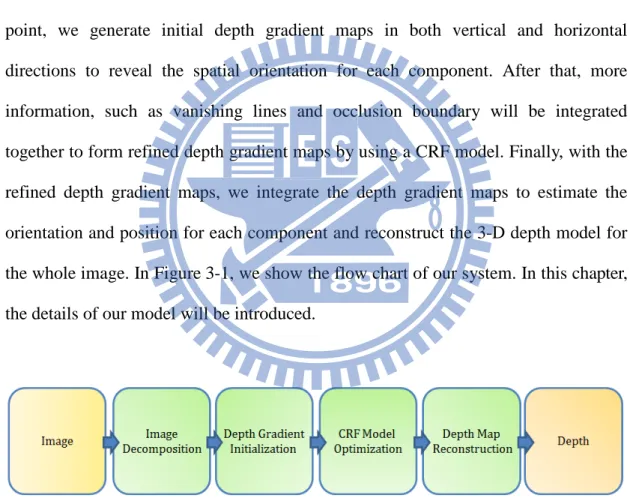
Our system starts from decomposing an image into several components. By classifying the components into different types, together with the estimated vanishing point, we generate initial depth gradient maps in both vertical and horizontal directions to reveal the spatial orientation for each component. After that, more information, such as vanishing lines and occlusion boundary will be integrated together to form refined depth gradient maps by using a CRF model. Finally, with the refined depth gradient maps, we integrate the depth gradient maps to estimate the orientation and position for each component and reconstruct the 3-D depth model for the whole image. In Figure 3-1, we show the flow chart of our system. In this chapter, the details of our model will be introduced.

Figure 3-1 Flowchart of our algorithm

3.1 Image Decomposition

In the aforementioned works [5-8, 12], either semantic labeling or geometric labeling can guide people to recover a depth map from a single image, relying on the

property of each label. In [11], the authors classify each region in the image into three geometric classes: ‘support’, ‘vertical’ and ‘sky’. We use the work in [11] by taking the advantage that these types have very different properties when assigning the depth value. The process starts from decomposing an image into several components and then classifies those components into three geometric types.

However, in [11], the authors use over-segmentation techniques and perform grouping recursively. The reason they use small regions is to prevent incorrect segmentation results and to collect useful cues, such as colors, textures, to reduce the probability of incorrect segmentation. In contrast, we apply the spectral matting method in [13, 14] to acquire image decomposition with larger spatial support. In our experiments, we found that ten to fifteen components are usually sufficient for the subsequent analyses.

In Section 3.3.1, we will briefly introduce the spectral matting method. In Section 3.3.2, we will introduce how we modify the spectral matting algorithm and show the matting results.

3.1.1 Image Matting with the Matting Laplacian

Spectral matting is introduced by Levin et al. in [13]. In their work, they generalize the compositing Equation (3.1) by assuming that each pixel i is a convex combination of K components F1, …, Fk : . , 0 1 where , 1 1 i a and a F a I ik K k k i K k k i k i i=

∑

∑

= ≥ ∀ = = (3.1)

The vectors αk are the matting components of the image, which represent the fractional contribution of each layer. They then find the smallest eigenvectors which correspond to the smallest eigenvalues of the Matting Laplacian matrix and utilize the

fact that to find the matting components is the same as to find a linear transform of these smallest eigenvectors. One example is shown in Figure 3-2.

(a)

(b) Figure 3-2 Example given by Levin et al.[13]. (a) Input Image. (b) Matting Components.

The Matting Laplacian is an affinity matrix specially designed for image matting. The key assumption of this approach is the color line model: the foreground and the background colors within a local image window ω around Pixel _i i lie on a single line in the RGB color space. Under this assumption, α value can be expressed as a linear transformation in the windowω . The description is written as: _i

b I a I a I a i∈ _i = R _iR + G _iG + B _iB+ ∀ ω a (3.2)

Here, i is index of the pixel,I ,_iR I_iG, and I_iB are values of the RGB channel, and a R_,

a G, a Band b as constants in the window.

Based on Equation (3.2), a cost function J(a,a,b) over all image windows can be defined as

. ) ( ) , , (

∑ ∑

G G B B 2 2 ∈ ∈ + − − − − = I q i w q q i q i q R i R q i q a b I a I a I a b a J a a ε (3.3)

A quadratic cost function of α is then denoted as . )

(a a La

J = T (3.4)

In Equation (3.4), L is called the matting Laplacian, which is a sparse symmetric positive semi-definite N×N matrix, and α is a N×1 vector, where N

is the number of image pixels. The matrix L is defined as the subtraction of a degree matrix D by an affinity matrixA; that is, L= D−A. Here, D is a diagonal

matrix, whose elements are defined asD(i,i)=

∑

N_j=1A(i, j). A is the sum of the matrices A_q, with the entries of A_q representing the affinities among pixels inside a

local window ω_q. That is, =

∑

qAq A and

(

)

(

)

      ∈         −         + − + = − otherwise. 0 ) ( 1 1 ) , ( 1 q q j q q T q i q q i,j j i ω ω ε ω I μ Σ U I μ A (3.5)

In Equation (3.5), I and _i I_j are the color values of the input image I at Pixels i and j,

q

μ is the 3×1 mean color vector of the image data in the window ω_q, Σ_q is a 3×3 covariance matrix in the same window, ω is the number of pixels within the window, _q and U is the 3×3 identity matrix [13].

in the image. This good property also provides global information for the whole image which will be used in later sections. Here, we provide an example of getting matting components by constructing the Matting Laplacian matrix via the method proposed by spectral matting. We take an image as input and set the matting component number as 10. (See Figure 3-3)

(a)

(b)

Figure 3-3 Result of Spectral Matting [13]. (a) Input Image. (b) Matting Components.

However, as we can see the results obtained by exploiting only color information are easily influenced by illumination. We use Figure 3-3 as an example to demonstrate the effect of incorrect area merging. In the left part of the original image, some cars and pedestrians are in front of a building. We expect they should be in different components, but the matting component result shows some parts are mixed. To make the image decomposition results more consistent, we make some modifications over the spectral matting algorithm.

3.1.2 Modification of Spectral Matting

The main idea of modification on spectral matting is to get additional channels besides RGB color channels when constructing the matting Laplacian matrix so we may get a more suitable decomposition. For example, though the road and the building are similar in color, they may be very different in texture. An intuitive choice of the additional channels is to choose appropriate texture features. In this thesis, we use Law’s filter mentioned in [15] to get the texture features. The measures are computed by filtering the image with small kernels and performing a moving-window to sum up the absolute values of the filter responses around each pixel.

We search for those texture filters that can be used to group pixels with similar properties. In [15], Law designed a set of filters to extract textures for the purpose of image segmentation. Law’s filter is composed of small convolution kernels, typically 5×5, which are generated from a set of 5x1 1-D convolution kernels. These 1-D convolution kernels stand for Level, Edge, Spot, and Ripple, as shown in Figure 3-4.

] 1 4 6 4 1 [ (Ripple) ] 1 0 2 0 1 [ ) Spot ( ] 1 2 0 2 1 -[ ) (Edge ] 1 4 6 4 1 [ (Level) 5 5 5 5 = = = = R S E L

Figure 3-4 1-D kernels of Law’s filter.

Each convolution kernel has different property. L5 is a center-weighted local

average, E5 detects edges, S5 detects spots, and R5 detects ripples. By combining the

1-D features, those kernels can achieve rotational invariance. To generate 2-D convolution kernels, we take one vertical 1-D kernel convolving with one horizontal 1-D kernel. For example, E5S5 kernel is produced by convolving a vertical E5 kernel

property of each channel, all convolution kernels used are zero-mean with the exception of the L5L5 kernel.

Figure 3-5 2-D masks of Law’s filter.

Those texture filters are applied to the test image to create 16 filtered images from which texture features are computed. After that, texture energies are computed by summing the absolute value of filtering results in each window. The 16 energy maps can be further reduced by combing similar filter pairs to produce 9 energy maps. For instance, E5L5 detects horizontal edges while L5E5 detects vertical edges. By averaging E5L5 and L5E5, rotational invariance is achieved. We apply Laws’ filters on our test image and Figure 3-6 shows the texture responses.

The resulting texture energy maps are treated as additional channels besides color channels. Now the terms in matting Laplacian matrix are extended as in Equation (3.6).

(

)

(

)

      ∈         −         + − + = − otherwise. 0 ) ( ' ' ' ' ' ' 1 1 ) , ( ' 1 q q j q q T q i q q i,j j i ω ω ε ω I μ Σ U I μ A (3.6)

Since there 9 texture channels added, we rewrite Equation (3.5) as Equation (3.6) in

order to show the difference in some terms. ForI'_i,I'_jand μ_q, we only need to extend the original 3x1 vector which indicate RGB color channels into a 12x1 vector

which cascades texture channels after color channels. Σ'_q is now a 12×12 covariance matrix in the same window, and U' is the 12×12 identity matrix.

The result of image decomposition after applying some modifications on spectral matting is shown in Figure 3-7.

Figure 3-7 Modified spectral matting with additional texture channels.

3.2 Initialization of Depth Gradient Maps

have the same trend in depth variation. We take each matting component as a planar surface. In this section we intend to infer the depth variation trend by classifying each component based on its geometric property and by detecting the position of vanishing point. Instead of assigning the depth value directly, we care about the depth variation between pixels which is called the depth gradient. In this section, the proposed method for the construction of depth gradient maps consists of three major steps: 1. matting component classification, 2. vanishing point detection, and 3. depth gradient map initialization. We will introduce each of them in the following subsections.

3.2.1 Matting component classification

To assign depth values according to object type, we classify each object into three geometric classes: ‘support’, ‘vertical’, and ‘sky’. Like other labeling works, we need some cues to estimate the geometric labels. In this step, we compute the appearance features in each matting component and find their geometric class. Here we use the surface layout approach [11] mentioned in Section 2.2. In their algorithm, there are 7 surface labels, including subclasses of ‘vertical’ class. The resulting maps present the likelihood of 7 possible classes. For convenience, all the maps are normalized to sum up as one. Though we plan to estimate the plane orientation for each component, we discard the use of subclasses maps. The likelihood for subclasses gives some confidence about the orientation of vertical classes. However, like other semantic labeling tasks, when classifying the image into more labels, classification accuracy in each subclass would be decreased. Hence, we only focus on the three main classes and Figure 3-8 shows the result.

(a) (b) (c) (d)

Figure 3-8 Result of Surface layouts. (a) Input Image. (b) Ground likelihood. (c) Vertical likelihood. (d) Sky likelihood.

For each region, we compute the average value of likelihood for each class, and find the maximum value among three classes which correspond to the most possible class. To illustrate the classification result, we use the matting components in Figure 3-7 as an example and its classification result is shown in Figure 3-9.

Figure 3-9 Geometric classification for the matting components in Figure 3-7.

3.2.2 Vanishing point detection

There are numerous research works that detect the vanishing point. However, it is not the main purpose of this thesis to go deep into this topic. We simply state the need of our problem and find an appropriate vanishing point detection method that fits our need.

of the urban image. Moreover, the algorithm should also work for clustered scenes to some extent. Many vanishing point detection algorithms use edge-based methods. They detect long lines in the image and find the intersections of lines to vote for the vanishing points. However, these algorithms are usually sensitive to spurious edges in the scene.

Kong et al. [16, 17] proposed a similar model but used texture orientation rather than the explicit line detection. In their approach, they first compute texture orientations for each pixel by using Gabor filters of different orientations. The texture orientation is chosen as the filter orientation which gives the maximum average complex response at each pixel, as shown in Figure 3-10 (b). They then determine the confidence of the orientation at each position. In Figure 3-10 (c), bighter pixels correspond to higher confidence in orientation estimation. A locally adaptive soft voting scheme is applied to find the most probable vanishing point in the image. In their algorithm, points around the upper part of the image are less favorable since vanishing point is less likely to appear there. We use the work proposed by Kong to obtain a more accurate vanishing point while pay more time to compute it. We show an example of their algorithm in Figure 3-10 (d).

(a) (b) (c) (d) Figure 3-10 Illustration of Kong’s algorithm [16, 17]:

3.2.3 Depth gradient maps initialization

After the detection of vanishing point, we attempt to blend the geometric information of vanishing point detection with these geometrically classified components to build up an initial 3-D geometric model. Here, we use a CRF model, which will be discussed in Section 3.3.

Up to now, though we still lack the absolute depth value for each pixel, we can estimate the rough orientation of each matting component based on the position of vanishing point. In this thesis, the depth gradients along the horizontal and vertical directions are modeled independently.

Here, we focus on components which are classified as vertical planes. Assuming there are no floating objects, all the ‘vertical’ components stand on the ground and their depth values are unchanged in the vertical direction. In contrast, the depth gradient along the horizontal direction is to be determined. Here, the horizon position of the vanishing point provides us the evidence about whether a vertical object is facing to the left or to the right of the viewer. More clearly, those components with their center on the left side of the vanishing point are likely to face right with respect to the viewer and those components on the right side of the vanishing point are likely to face left. Figure 3-11 illustrates this idea.

Figure 3-11 Geometric information provided by vanishing point for ‘vertical’ regions.

planner surface, which is almost parallel to the horizon of our view in the world coordinates. As we move closer to the position of vanishing point the depth value increases, as shown in Figure 3-12. For the sky region, since it is always the farthest in an image, we ignore its depth gradient and simply assign zero values for this region.

Figure 3-12 Geometric information provided by vanishing point for ‘ground’ regions.

Now, we explain the definition of labeling rule for the depth gradient maps in the horizontal and vertical directions. For horizontal depth gradient map, we consider the direction of depth gradient to be from left to right. Here, we use discrete labels, instead of computing real-value depth gradient values, in order to make the assignment fast and simple. We only consider the possible trends of depth gradient by classifying all possible values into five groups. Components with its orientation facing to the right means their depth increases as getting closer to the vanishing point. Since we get positive depth gradients for these components, this type is named as ‘increase continuously’. In the same way, for components whose depth decrease in the horizontal direction are named as ‘decrease continuously’. Besides, zero depth gradient components are named as ‘unchanged’.

Additionally, until now we have discussed those cases with gradual changes in depth and the case with zero depth gradients. However, there are some boundaries between different components at which we expect the depth value will change

abruptly. Hence, we define two additional labels, named as ’increase abruptly’ and ‘decrease abruptly’.

Now we consider the labels for the depth gradient map in the vertical direction. In the vertical direction, ‘vertical’ components are labeled as ‘unchanged’ since they stand on the ground and have a constant depth value. For the ground region, it is a planar surface and its depth increases as getting closer to the vanishing point. Hence, we label the ground region as ‘increase continuously’. In fact, the depth ordering of the objects with respect to the camera viewpoint will be consistent with the projected components in the image. Those components at lower positions in the image often occlude those at higher positions. With this assumption, all the boundaries will be assigned the ‘increase abruptly’ label. In Figure 3-13, we illustrate the labeling result of the initial depth gradient maps in different gray-levels.

Figure 3-13 Initial labeling of depth gradient maps. (a) Input Image. (b) Depth gradient map in the horizontal direction. (c) Depth gradient map in the vertical direction.

3.3 CRF Model Optimization

Up to now, we have obtained the initial depth gradient maps by using the geometric classification results of surface layout geometric classification and the

(a) (b) (c)

geometric cues constrained by the vanishing point. This can be regarded as the initial geometric model of the image. However, there are some other issues that we have not considered yet.

One concern is about the occlusion boundaries. Occlusion boundary refers to the boundary where a scene occlusion occurs. That is, the occluding object blocks the views of the occluded objects behind it. In Section 3.1.2, we have handled the problem that at matting boundaries the result may be blended with adjacent components through adding texture channels. However, it is still not enough to distinguish occlusion boundaries that are between different objects from those boundaries that are actually not between two different objects. Figure 3-14 gives an example.

Figure 3-14 An example of non-occlusion boundaries.

Another concern is the orientation of ‘vertical’ components. In the previous step, we simply assign their labels with one of two possible situations: either facing-left or facing-right. Nevertheless, it is also possible for a ‘vertical’ component to face right in front of the camera, like the building and the cars in the orange rectangles in Figure 3-15. Here, we attempt to take this case into consideration.

Figure 3-15 Examples of facing-front ‘vertical’ components.

In the following sections, we will handle the issues mentioned above which employ extra geometric constraints on orientation estimation and boundary detection. Moreover, we want to use a graphical model to obtain a global solution for depth gradient reasoning based on the extra information provided by geometric constraints and boundary detection algorithm. This model is a conditional random field (CRF) model which will be introduced in later sections. In Section 3.3.1, the occlusion boundary algorithm is introduced. In Section 3.3.2, we detect vanishing lines in three main directions which will be used as geometric constraints for object orientation estimation. In Section 3.3.3 and Section 3.3.4, we will describe the adopted CRF model and state how we formulate our problem by using the CRF model.

In this section, we will first demonstrate the result we want to obtain. The example in

Figure 3-16 illustrates how a CRF model can improve the global consistency of the depth gradient map labeling.

Figure 3-16 Horizontal direction: (a) Initial depth gradient map. (b) Refined depth gradient map. Vertical direction: (c) Initial depth gradient map. (d) Refined depth gradient map.

3.3.1 Occlusion boundary

Our work for finding occlusion boundaries is mainly inspired by Hoiem’s works in [6, 7]. Since the appearance of objects may be inhomogeneous and may consist of different color/texture regions, it is not so straightforward to distinguish occlusion boundaries from non-occlusion boundaries. In Hoiem’s work, they estimate depth from image segmentation and perform figure/ground assignment using machine learning techniques. In our case, some modifications will be made over their approach to deal with images of urban scenes.

Here, we make a briefly review of Hoiem’s work. Their algorithm starts from over-segment the image first and then recursively remove those unlikely edges to get the final boundaries. Depending on the region size, their classification algorithm consists of three stages to learn different classifiers with different features. In the third stage, they use features which measures over a larger spatial support besides local features. The algorithm does the merging process iteratively in the third stage by setting a threshold over the occlusion boundary likelihood value until no more components can be merged.

In our work, the number of matting component is typically ten to fifteen whose region is large enough to obtain valuable spatial information. We consider eliminating the first and second stages in their occlusion boundary algorithm and use the third stage classifier only. We take the matting components as the input and measure occlusion cues within each matting component. Through this process, we get the measures of boundary information while maintaining the boundaries generated by matting. After that, we use the occlusion boundary classifier in the third stage of Hoiem’s work and get the result of occlusion boundaries. Figure 3-17 shows an example of the detected boundaries. In the left figure, the white lines typified the original boundary map. In the right figure, we show the result of occlusion boundary in which some non-occlusion boundaries are removed. In the image, the component to the left of an arrow is in front of the component to the right of the arrow.

(a) (b)

Figure 3-17 (a) Original boundary map (b) The result of using occlusion boundary algorithm [6, 7].

3.3.2 Vanishing line detection

Though Hoiem used vanishing line cues to obtain the surface layout, they mainly use the vanishing line information to detect vertical/support surface. In this thesis, our goal is to find the vanishing lines which can be classified into three main groups: vertical, horizontal and lean. Besides, since we have detected the vanishing point associated with the main road as mentioned in Section 3.2.2, the detected vanishing

lines can help to construct the depth gradient maps in both horizontal and vertical directions.

In our approach, we use the conventional edge-based method to detect vanishing lines. This method is a part of the work proposed by Tardif et al. in [18]. In Tardif et al.’s method, they use the canny edge detector to extract pixel edges and then use Hough transform to detect straight lines. In Figure 3-18, we use random colors to denote different orientations of vanishing lines. In the example shown in Figure 3-18, blue color lines are vertical vanishing lines, green color lines are lean vanishing lines and orange color lines are horizontal vanishing lines.

Figure 3-18 Three main groups of vanishing lines.

3.3.3 CRF Model Introduction

We aim to use a model to enablejoint inference over initial depth gradient labels, occlusion boundary likelihood, and geometric constraint to enforce a more reasonable and consistent depth map.

A solution to this problem is to directly model the conditional distribution

) | (y x

p , which can be used to classify each pixel by the most likely depth gradient label. In [19], John et al. first introduced the CRF(conditional random fields) model. A conditional random field model is simply a conditional distribution p(y|x) with an associated graphical structure.

of labels given an observation sequence. This model can be characterized by the energy functions with two terms: unary and pairwise term, which are written as:

∑

∑

∈ ∈ + = εψ νψ (, ) ) , ( ) ( ) ( j i j i ij i i i x D x x D E x (3.7)

In Equation (3.7), D denotes the observation sequence, ν corresponds to the set of all image pixels, and

ε

is the set of connecting edges of pixels, withi, j∈ν. Sometimes, the notation D will be ignored to simplify the formulation. The random variable x denotes the labeling of pixel _i i on the image. Any possible assignment of labels is denoted as

x

, which takes values from the labeling setL. The first term in

) (x

E is the unary term which models the negative log of the likelihood of a label being assigned to the pixeli. Pairwise term ψ takes a contrast sensitive Potts _ij model in which the cost is nonzero if neighboring pixel i and pixel j takes different labels, as expressed in Equation (3.8). g( ji, ) _{can be any function which}

measures the difference between neighboring pixels.

   = = otherwise , ) , ( , 0 ) , ( j i g x x x x_{i j} i j ij ψ (3.8)

For the CRF model, each x_i∈x is associated with a pixel i∈ν and will take an optimal assignment from the labeling setL. The corresponding solution can be solved by finding the minimum energy of the CRF model. This is actually a maximum a posteriori (MAP) estimation problem which can be denoted as

) x ( min arg ) | x ( x max arg x* P D E x = = (3.9)

The CRF model proposed by John et al. relates neighboring pixels only. However, since this model lacks long range interaction, researchers recently proposed

methods to extend the model to enables consistency in a region. In [20], Kohli et al. proposed a method which allows the integration of multiple region-based CRF’s with a low-level pixel-based CRF and eliminate those inconsistent regions. Equation (3.10) shows their model:

∑

∑

∑

∈ ∈ ∈ + + = s D x x D x E c c c j i j i ij i i i( ) ( , ) ( ) ) ( ) , ( x x ψ εψ νψ (3.10)

The first two terms are the same as the original CRF model proposed by Lafferty et al., while the third term, called the region consistency potential term, allows the CRF model to be more flexible. The region consistency potential favors the case when all pixels of a component take the same label. In the third term of Equation (3.10), S

is a set of all possible image segmentations and the term ψ_c the corresponding higher order potential defined on those segmentations. ψ_c is also called the higher order potential term.

More formulation details about the CRF model will be explained in Section 3.3.4. We use an example here to show one of Kohli’s results which applied the CRF model to object segmentation and recognition problem. In Figure 3-19, (a) is an image for testing and (b) to (d) shows multiple segmentations of the image by using different thresholds. Figure 3-19 (h) is a hand-labeled result used as ground truth. Figure 3-19 (e), (f), (d) show the result of using unary potentials only, using pair-wise CRF model , and using the higher order CRF model, respectively, for comparison. Figure 3-19 (e) is the labeling result by using the unary likelihood potentials from textures. This often gets broken result. By using the pair-wise CRF model, it enforces label consistency of adjacent pixels. However, the result assigns the bird’s leg to the ‘water’ label. Figure 3-19 (g) shows the solution of the higher order CRF. In Figure 3-19 (b) and (c), the

segmentation result only contains the leg of bird. Since it is surrounded by water region, it is likely to be labeled as ‘water’. However, with multiple-segmentations, it will get a higher cost for the third term when the two different labels ‘water’ and ‘birds’ are assigned to the pixels of the bird. This causes the leg of the bird to be properly reserved.

Figure 3-19 Object segmentation and recognition using the CRF higher order Model.

3.3.4 Formulation of CRF Model

In this section we will describe how to formulate our problem into a CRF model. As mentioned above, the higher order model is able to achieve label consistency in a region. In our case, we aim to do a pixel-wised labelling problem while maintaining the consistency of region label. Hence, the higher order model is suitable for us to take it as a part of the prototype of system. In the following, we will show how we integrate all the information to help the assignment of depth gradient maps.

First of all, we formulate the model with a set of nodes, which correspond to the

total number of pixels of the input image, and a labeling setL={l₁,l₂,l₃,l₄,l₅}

, which corresponds to the five possible depth gradient values.

Unary potential term

The unary potential is often defined as the negative log of the likelihood of a label being assigned to a pixel. In our model, we get an initial depth gradient map which assigns the most likely label for each pixel. Moreover, we can also propagate the likelihood term from the most likely label to other labels through a reasonable

guess.

We first interpret how we define the cost based on the relationship between possible labels. For Pixel i with the label ‘decrease abruptly’, it may be on a non-occluded/occlusion boundary in real situation. Hence, it comes out to have two other possible labels: ‘unchanged’ and ‘decrease continuously’ whereas there is little chance for Pixel i to have an increasing depth since this case often appears on the other side of image. So the cost of being labeled as ‘increase continuously’ and ‘increase abruptly’ is large. The same idea also applied on pixel i with label ‘increase abruptly’ which only differs from the previous case in the changing direction.

Another case is Pixel i with label ‘decrease continually’. It may be the case that actually there is a planar surface facing the front, so ‘unchanged’ could be a second choice. We set all other labels with same cost value. The same manner also applied for ‘increase continually’ label.

The possible situations for ‘unchanged’, is for those pixels on horizontal vanishing lines. For this case, we force those pixels to have ‘unchanged’ label by giving high costs for other labels.

After that, we construct the cost plane which defines the penalty of assigning

label l_k to pixel i which is initialized as label l . The dimension of the cost plane _m

will be (number of possible labels) x (number of image pixels). The unary potential term then consists of the sum over all pixels i of the cost plane, this can be written

as

ψ

i(xi)= p(xi∈lm | xi ∈lk)_.

The definition of p(xi ∈lm |xi ∈lk) is in Figure 3-20 Here we use a table to

and W₃ are the weighting costs which we set W1 as 0.5, W2 as 5, and W3 as 10 in

this thesis.

Figure 3-20 Label cost in the label set based on the initial labeling guess.

Pairwise term

The pairwise terms ψ_ijof the CRF is typically defined as an edge feature based on the color difference of a 4-neighborhood or 8-neighborhood pixel pair. Instead of using the conventional definition, we define it by using the Matting Laplacian matrix, which has been used to generate Matting components. The Matting Laplacian matrix describes the connectivity between adjacent pixels in an image. The use of Matting Laplacian matrix provides the global information of the whole image and there is no need to compute the pairwise term again. Here, we show the definition of matting Laplacian again in Equation (3.11):

    = = =

∑

,otherwise ) , ( , 0 ) , ( q q j i j i ij A j i g x x x x ψ (3.11)

(

)

(

)

      ∈           −         + − + = − otherwise. 0 ) ( 1 1 1 q q j q q T q i q q i,j A where ω ω ε ω I μ Σ U I μ

Region-based consistency potential

form mentioned in Kohli’s work. This potential term is expressed in Equation (3.12)     _≤ = otherwise. , Q ) i( if 1 ) ( ) ( max max γ γ ψ i c c c c N Q N x x x (3.12)

The behavior of Equation (3.12) is shown in Figure 3-21.

Figure 3-21 Behavior of the region based consistency potential term.

In Equation (3.12),c∈S, where S is the set of all the possible segments of an image. N x_i( _c) denotes the number of variables in the segment c that which are not

taking the dominant label and Q controls the rigidity of the region-based

consistency potential term. In other words, the definition allows pixels within a segment to have different labels if the amount of pixels which taking other labels than the dominant one is greater than Q. γ_maxhere is a predefined threshold, whose value depends on each label.

We use an example to illustrate the role of the region-based consistency potential. In our model, one set of segments is the matting components got from spectral matting, and the other set of segments is the result of Hoiem’s occlusion boundary algorithm using matting components as the input. We show one example in Figure 3-22 which show the two sets of possible segments in our experiment. The main difference between these two segmentations is over the building region in the right

part of the image. Originally, the building was divided into three components by using the spectral matting algorithm. After removing occlusion boundaries, the three components are merged into one single component.

(a) (b) (c)

Figure 3-22 Set of possible segmentation. (a) Input Image. (b) Matting components. (c) Result after using occlusion boundary algorithm in [6, 7] (Use different colors to represent different

segments for visualization)

Since the boundaries on the initial depth gradient maps corresponds to the boundaries for the regions in Figure 3-22(b), the maps may only deal with a few points in a region which take different labels other than the major labels. In Figure 3-23, for the region in the orange box, the majority of labeling is ‘decrease continuously’. There are some points which are originally labeled as ‘decrease

abruptly’ to represent for boundary. They will be considered asN_i (x_c) in Equation (3.12). In the definition of Equation (3.12), these points labels as’ decrease abruptly’ will contribute some cost.

Figure 3-23 Example of how region consistency works to remove non-occlusion boundary. (a) Segmentation map. (b) Initial depth gradient map in the horizontal direction.

As all the energy functions are defined for our CRF model, a graph cut based expansion and swap-move algorithm can be used to lower the energy recursively to get the final optimal solution. By using Kohli’s optimization algorithm, we get the optimized depth gradient maps. (See Figure 3-24)

(a) (b) (c)

Figure 3-24 Refined depth gradient maps. (a) Original Image. (b) Horizontal direction. (c) Vertical direction.

3.4 Reconstruction of Depth Map

Until now, we have built up the depth gradient maps by using the CRF model and also the estimated orientation for every component in the image. It means we are ready to construct the 3-D depth. At the last stage, we attempt to reconstruct the depth map image through the optimized depth gradient maps in both horizontal and vertical directions. We will first go through the camera model which helps us to better understand the image plane and its relationship with the world coordinates. After that, we introduce how to estimate the depth values for each component based on the depth gradient maps.

3.4.1 Camera Model

In [6, 7], Hoiem et al. propose a zero-skew, unit aspect ratio, perspective model. Here we use the same camera model to estimate 3D object locations. By assuming

that all objects rest on the ground, given the horizontal lines in image and the camera height we can estimate the 3D distance of the object with respect to the camera center. The derivation of object location equations is mentioned in [21].

We first define some notations as follows: pixel coordinates (u,v) in an image is normalized, with(0,0)at the top-left and(1,1)is at the bottom-right. (uc,vc)is the camera center in the image, and the horizon position of the vanishing point is named

asv0. In the world coordinates, we use the notation(x,y ,z)_{, where}

z

refers to the depth andyis the object height. The camera center is defined as the origin of the

world coordinates. The ground plane hasy=0. The camera height isy_c. Besides, f

is the focal length and θ is the tilt angle of the camera. _x

With the assumptions of zero skew and unit aspect ratio, the transformation from the world coordinates to the image coordinates can be written as

                                =           1 0 cos in 0 in cos 0 0 0 0 1 1 0 0 0 0 1 1 z y x s y s v f u f z v u x x c x x c c θ θ θ θ (3.13)

By solving the equation above, we have

𝑦 =𝑧(𝑣−𝑣𝑐cos 𝜃𝑥+𝑓 sin 𝜃𝑥)−𝑓𝑦𝑐

𝑓 cos 𝜃𝑥+𝑣𝑐sin 𝜃𝑥 , and (3.14) 𝑥 =𝑢∙𝑧−𝑢𝑐(𝑦 𝑠𝑠𝑠 𝜃𝑥+𝑧 𝑐𝑐𝑠 𝜃𝑥)

𝑓 . (3.15)

Denote the bottom position of an object as (ub,vb).Since we have the assumption that the object is on the ground, we havey=0. By plugging Equation (3.15) with u =u_b