國立交通大學
資訊科學與工程研究所
博 士 論 文
在串流資料中高效率頻繁樣式探勘演算法之研究
A Study of Efficient Mining Algorithms of Frequent
Patterns on Data Streams
研 究 生:李華富
指導教授:李素瑛 博士
在串流資料中高效率頻繁樣式探勘演算法之研究
A Study of Efficient Mining Algorithms of Frequent
Patterns on Data Streams
研 究 生:李華富 Student:Hua-Fu Li
指導教授:李素瑛博士 Advisor:Dr. Suh-Yin Lee
國 立 交 通 大 學
資 訊 科 學 與 工 程 研 究 所
博 士 論 文
A Dissertation
Submitted to Department of Computer Science College of Computer Science
National Chiao Tung University in partial Fulfillment of the Requirements
for the Degree of Doctor of Philosophy
in
Computer Science June 2006
Hsinchu, Taiwan, Republic of China
i
在串流資料中高效率頻繁樣式探勘演算法之研究
在串流資料中高效率頻繁樣式探勘演算法之研究
在串流資料中高效率頻繁樣式探勘演算法之研究
在串流資料中高效率頻繁樣式探勘演算法之研究
學生:李華富 指導教授
:李素瑛博士
國立交通大學 資訊科學與工程研究所
摘要
資料串流探勘是一個快速成長的新興研究領域,但同時也帶來了新的挑戰。在眾多資料串 流探勘的研究中,頻繁樣式探勘與變化探勘一直是資料串流探勘中重要的研究焦點。本論 文主旨在於研發高效率的頻繁項目集合、路徑瀏覽樣式,以及項目變化樣式的單次線上掃 描探勘方法。頻繁項目集合是本論文所探討的第一個研究主題。首先,針對串流資料的標的物模型, 我們提出一個可快速地探勘出所有頻繁項目集合的單次掃描演算法 DSM-FI。為了避免將每 一筆新進交易中所有項目集組合都窮舉出來,我們設計了一個有效的交易投影機制,並提 出一個新的摘要字首樹狀結構來儲存必要的集合項目資訊。此演算法在探勘出頻繁項目集 合的同時,也可找出最大頻繁項目集合。 我們也針對串流資料的滑動窗模型提出了兩個單次頻繁項目集合探勘演算法 MFI-TransSW與 MFI-TimeSW,可有效地在交易感知滑動窗模型以及時間感知滑動窗模型 中探勘出目前存在的頻繁項目集合。MFI-TransSW 與 MFI-TimeSW 演算法主要是利用位元 向量的特性來儲存單一項目在目前滑動窗中的出現位置,並利用位元向量的特性來達到快 速滑動的效果。
ii 路徑瀏覽樣式是本論文所探討的第二個主題。我們提出可快速探勘出路徑瀏覽樣式的 單次掃描演算法 DSM-PLW,此演算法沿用 DSM-FI 的精神,利用快速拆解使用者瀏覽路 徑,以及字首樹狀結構的特性,來達到串流資料探勘的效能要求。此外,我們進一步提出 一個不需要使用者輸入最小支持度門檻值,就可以進行的 Top-K 路徑瀏覽樣式的單次掃描 探勘演算法。 串流資料變化探勘是本論文的第三個研究主題。我們提出 MFC-append 演算法來找出 在兩條線上交易資料串流中,穩定分布的交易項目、常常變動的項目,或無一定分佈的變 化樣式。此外,針對可執行刪除運算的動態資料串流,我們提出一個以 MFC-append 為基 礎的演算法 MFC-dynamic,來探勘動態資料串流中的項目變化。 我們進行了相關的實驗以評估所提方法的效能。在我們的實驗範圍中的結果顯示,對 於各個不同探勘參數以及不同特性的資料集,我們的方法都優於許多著名的方法。此外, 針對資料量擴充的實驗也顯示出我們所提出的探勘頻繁樣式的方法具有線性的擴充能力。
iii
A Study of Efficient Mining Algorithms of Frequent
Patterns on Data Streams
Student:Hua-Fu Li Advisor:Dr. Suh-Yin Lee
Department of Computer Science
National Chiao Tung University
Abstract
Online mining of data streams is an important data mining problem with broad applications. However, it is a difficult problem since the streaming data possess some specific characteristics, such as unknown or unbounded length, possibly very fast arrival rate, inability to backtrack over previously arrived transactions, and a lack of system control over the order in which data arrives. Among various objectives of data stream mining, the mining of frequent patterns in data streams has been the focus of knowledge discovery. In this dissertation, the design of several core technologies for mining frequent patterns and changes of data streams is investigated.
For mining of frequent itemsets over data streams with a landmark window, we propose the DSM-FI (Data Stream Mining for Frequent Itemsets) algorithm to find the set of all frequent itemsets over the entire history of the data streams. An effective projection method is used in the proposed algorithm to extract the essential information from each incoming transaction of the data streams. A data structure based on prefix tree is constructed to store data summary. DSM-FI utilizes a top-down pattern selection approach to find the complete set of frequent itemsets. Experiments show that DSM-FI outperforms BTS (Buffer-Trie-SetGen), a state-of-the-art
iv
single-pass algorithm, by one order of magnitude for discovering the set of all frequent itemsets over a landmark window of data streams.
For mining of frequent itemsets in data streams with a sliding window, efficient bit vector based algorithms are proposed. Two kinds of sliding windows, i.e., transaction-sensitive sliding window and time-sensitive sliding window, are discussed. MFI-TransSW (Mining Frequent Itemsets over a Transaction-sensitive Sliding Window) is developed to mine the set frequent itemsets over data streams with a transaction-sensitive sliding window. A single-pass algorithm, called MFI-TimeSW (Mining Frequent Itemsets over a Time-sensitive Sliding Window), based on MFI-TransSW algorithm and a dynamic encoding method is proposed to mine the set of frequent itemsets in a time-sensitive sliding window. An effective bit-sequence representation of items is used in the proposed algorithms to reduce the time and memory needed to slide the windows. Experiments show that the proposed algorithms not only attain highly accurate mining results, but also run significantly faster and consume less memory than existing algorithms for mining recent frequent itemsets over data streams.
For mining changes of items across two data streams, we propose two one-pass algorithms, called MFC-append (Mining Frequency Changes of append-only data streams) and MFC-dynamic (Mining Frequency Changes of dynamic data streams), to mine the set of frequent frequency changed items, vibrated frequency changed items, and stable frequency changed items across two continuous append-only and dynamic data streams, respectively. A new summary data structure, called Change-Sketch, is developed to compute the frequency changes between two data streams as fast as possible. Theoretical analysis and experimental results show that our algorithms meet the major performance requirements, namely single-pass, bounded space requirement, and real-time computing, in mining data streams.
v
Mining path traversal patterns from Web click streams is important in Web usage mining and Web user profiling. One of the most important We proposed two single-pass algorithms, called DSM-PLW (Data Stream Mining for Path traversal patterns in a Landmark Window) and DSM-TKP (Data Stream Mining for Top-K Path traversal patterns), to discover the path traversal patterns over Web click-streams with and without a user-defined minimum support constraint. Experiments of real data show that both algorithms successfully mine maximal reference sequences with linear scalability.
Comprehensive experiments have been conducted to assess the performance of the proposed algorithms. The empirical results show that these algorithms outperform the state-of-the-art algorithms with respect to various mining parameters and datasets of different characteristics. The scale-up experiments also verify that our algorithms successfully mine frequent patterns with good linear scalability.
vi
Acknowledgement
(
(
(
(誌謝
誌謝
誌謝
誌謝)
)
)
)
首先,我最感謝的是我的指導教授李素瑛老師,感謝她在這五年的研究所生涯中啟發我對 學術研究的興趣,並且指導我論文的寫作上的技巧,以及生活上的幫助。在跟隨李老師研 究的過程中,李老師對研究的執著及熱忱,一直是我學習的榜樣。此外,還要感謝孫春在 教授和彭文志教授在計劃書口試、校內口試以及校外口試時提供許多寶貴的意見。 感謝口試委員:台大電機系陳銘憲教授、成大資工曾新穆教授、中央資工系張嘉惠教 授、政大資科系沈錳坤教授在口試過程中提供許多寶貴的建議,讓我的論文能更趨完善。 諸位口試委員都是我在學術研究的道路上的最佳學習典範。 資訊系統實驗室的學長與學弟妹是我博士班研究生涯的好伙伴,謝謝大家也祝福學弟 妹們早日收穫豐富的研究成果。再次謝謝你們在這段過程中對我的幫忙及鼓勵。 一直陪伴在我身旁、沒有怨言、只給我鼓勵的,就是我的太太佑青。能夠順利完成博 士學位,對於佑青,我有無盡的感謝。 要感謝的人太多,僅在此對所有曾經幫助過我的朋友,致上我真切的謝意。 僅以此論文,獻給我摯愛的太太佑青。vii
Table of Contents
Abstract in Chinses... i
Abstract in English ... iii
Acknowledgement... vi
List of Figures ... ix
Chapter 1 Introduction ... 1
1.1 Background... 1
1.2 Research Objectives and Contributions... 3
1.3 Organization of this Thesis... 4
Chapter 2 Online Mining of Frequent Itemsets in Data Streams ... 6
2.1 Introduction ... 7
2.2 Problem Definition ...11
2.3 The Proposed Algorithm: DSM-FI ... 13
2.3.1 Construction and Maintenance of Summary Data structure... 13
2.3.2 Pruning Infrequent Information from SFI-forest... 19
2.3.3 Determining Frequent Itemsets from Current SFI-forest... 22
2.4 Theoretical Analysis ... 25
2.4.1 Maximum Estimated Support Error Analysis... 25
2.4.2 Space Requirement Analysis... 26
2.5 Performance Evaluation ... 27
2.5.1 Scalability Study of DSM-FI Algorithm... 28
2.5.2 Comparison with BTS algorithm... 30
2.6 Conclusions ... 30
Chapter 3 Online Mining of Frequent Itemsets over Stream Sliding Windows ... 32
3.1 Introduction ... 33
3.2 Problem Definition: Mining Frequent Itemsets in a TransSW ... 34
3.3 The Proposed Algorithm: MFI-TransSW ... 36
3.3.1 Bit-Sequence Representation... 36
3.3.2 The MFI-TransSW Algorithm... 37
3.3.2.1 Window Initialization Phase... 37
3.3.2.2 Window Sliding Phase... 38
3.3.2.3 Frequent Itemsets Generation Phase... 40
3.4 Problem Definition: Mining Frequent Itemsets in a TimeSW... 41
3.5 The Proposed Algorithm: MFI-TimeSW... 43
3.5.1 Time Unit List and Bit-Sequences of Items... 43
3.5.2 The MFI-TimeSW Algorithm... 44
3.5.2.1 Window Initialization Phase... 44
3.5.2.2 Window Sliding Phase... 45
3.5.2.3 Frequent Itemsets Generation Phase... 45
3.6 Performance Evaluation ... 49
3.6.1 Experiments of MFI-TransSW Algorithm... 50
3.6.2 Experiments of MFI-TimeSW Algorithm... 54
3.7 Conclusions ... 55
viii
4.1 Introduction ... 56
4.2 Related Work ... 58
4.3 Problem Definition: Mining of Changes of Items across Two Data Streams... 58
4.4 Online Mining Changes of Items over Distributed ADSs ... 61
4.4.1 A New Summary Data Structure: Change-Sketch... 61
4.4.2 The MFC-append Algorithm... 62
4.4.3 Space Analysis of Change-Sketch... 66
4.5 Online Mining Changes of Items over Distributed DDSs ... 67
4.6 Performance Evaluation ... 68
4.6.1 Synthetic Data Generation... 68
4.6.2 Experimental Results... 70
4.7 Conclusions ... 72
Chapter 5 Online Mining of Path Traversal Patterns over Web Click-Streams... 74
5.1 Introduction ... 74
5.2 Problem Definition: Online Mining of Path Traversal Patterns ... 78
5.3 The Proposed Algorithm: DSM-PLW ... 79
5.3.1 Construction of the In-memory Summary Data Structure... 80
5.3.2 Pruning Mechanism of the Summary Data Structure... 86
5.3.3 Determination of Path Traversal Patterns from SP-forest... 88
5.4 Performance Evaluation ... 89
5.4.1 Experimental Results of Synthetic Data... 90
5.4.2 Experimental Results of Real Data... 96
5.5 Conclusions ... 96
Chapter 6 Online Mining of Top-K Path Traversal Patterns over Web Click-Streams... 98
6.1 Introduction ... 98
6.2 Problem Definition ... 99
6.3 The Proposed Algorithm: DSM-TKP ... 100
6.3.1 Effective Construction of the Summary Data Structure... 101
6.3.2 Effective Pruning of the Summary Data Structure... 105
6.3.3 Determination of the Top-K Path Traversal Patterns... 106
6.4 Performance Evaluation ... 106
6.5 Conclusions ... 107
Chapter 7 Conclusions and Future Work ... 109
7.1 Conclusions ... 109
7.1.1 Summary of Mining of Frequent Itemsets in Data Streams... 109
7.1.2 Summary of Mining of Frequent Itemsets over Stream Sliding Windows...110
7.1.3 Summary of Mining of Changes of Items across Two Data Streams...110
7.1.4 Summary of Mining of Path Traversal Patterns over Web Click-Streams....111
7.1.5 Summary of Mining of Top-K Path Traversal Patterns...111
7.2 Future Work ...111
References...113
Publication List ... 120
ix
List of Figures
Figure 2- 1. Typical processing model of data streams ... 7
Figure 2- 2. Algorithm SFI-forest Construction ... 16
Figure 2- 3. Subroutines of SFI-forest construction algorithm ... 18
Figure 2- 4. SFI-forest construction after processing the first transaction < acdf >... 18
Figure 2- 5. SFI-forest construction after processing the second transaction < abe > ... 19
Figure 2- 6. SFI-forest construction after processing the window Wj... 20
Figure 2- 7. SFI-forest after pruning all infrequent items ... 21
Figure 2- 8. Algorithm todoFIS ... 24
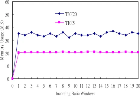
Figure 2- 9. Resource requirements of DSM-FI algorithm for IBM synthetic datasets: (a) execution time, (b) memory usage ... 29
Figure 2- 10. Comparison of DSM-FI and BTS: (a) Execution time, (b) Memory Usage... 30
Figure 3- 1. Transaction-sensitive sliding window and time-sensitive sliding window [51] ... 32
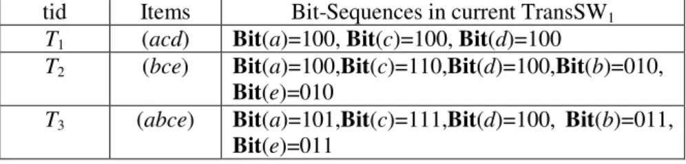
Figure 3- 2. An example transaction data stream and the frequent itemsets over two consecutive TransSWs... 35
Figure 3- 3. Bit-sequences of items in window initialization phase of TransSW ... 37
Figure 3- 4. Bit-sequences of items after sliding TransSW1 to TransSW2... 37
Figure 3- 5. Algorithm MFI-TransSW... 39
Figure 3- 6. Steps of frequent itemsets generation in TransSW2... 40
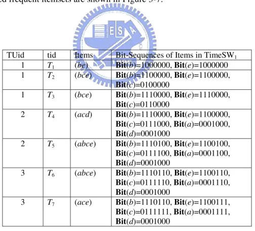
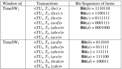
Figure 3- 7. An example transaction data stream and the frequent itemsets over two time-sensitive sliding windows... 43
Figure 3- 8. Bit-sequences of items in window initialization phase of TimeSW1... 46
Figure 3- 9. Bit-sequences of items after sliding TimeSW1 to TimeSW2... 47
Figure 3- 10. Algorithm MFI-TimeSW ... 48
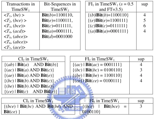
Figure 3- 11. Steps of frequent itemsets generation of MFI-TimeSW in TimeSW1... 49
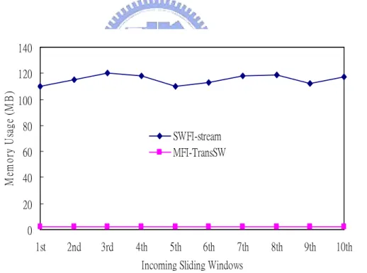
Figure 3- 12. Memory usages in window initialization phases of algorithms SWFI-stream and MFI-TransSW (s = 0.1% and w = 20,000) ... 51
Figure 3- 13. Memory usages in window sliding phases of algorithms SWFI-stream and MFI-TransSW (s = 0.1% and w = 20,000) ... 51
x
Figure 3- 14. Memory usages in frequent itemset generation phases of algorithms SWFI-stream
and MFI-TransSW (s = 0.1% and w = 20,000) ... 52
Figure 3- 15. Processing time in window initialization phases of algorithms SWFI-stream and MFI-TransSW under different window sizes (s = 0.1%) ... 52
Figure 3- 16. Processing time including window sliding time and pattern generation time of algorithms SWFI-stream and MFI-TransSW under window size 200K transactions (s = 0.1%) ... 53
Figure 3- 17. Memory usages of MFI-TimeSW algorithm in different phases (s = 0.1%) ... 53
Figure 3- 18. Processing time of MFI-TimeSW algorithm in different phases (s = 0.1%) ... 54
Figure 4- 1. Processing model of distributed data streams... 57
Figure 4- 2. Examples of VFCIs and SFCIs ... 60
Figure 4- 3. Notations and conventions used in the proposed algorithms... 63
Figure 4- 4. Algorithm MFC-append ... 64
Figure 4- 5. Algorithm MFC-dynamic ... 69
Figure 4- 6. Experiments on synthetic data (104 transactions) for MFC-append. Left: recall (proportion of the frequent change patterns reported). Right: precision (proportion of the output frequency change patterns which are frequent)... 70
Figure 4- 7. Experiments on synthetic data (105 transactions) for MFC-append. Left: recall. Right: precision ... 71
Figure 4- 8. Experiments on synthetic data (106 transactions) for MFC-append. Left: recall. Right: precision ... 71
Figure 4- 9. Experiments on synthetic data (106 transactions) for MFC-dynamic. Left: recall. Right: precision ... 72
Figure 5- 1. Process of online mining of path traversal patterns in Web click streams... 79
Figure 5- 2. Algorithm SP-forest construction ... 82
Figure 5- 3. Subroutines of SP-forest construction algorithm... 83
Figure 5- 4. SP-forest after processing the first maximal forward reference <acdef> ... 84
Figure 5- 5. SP-forest after processing the second maximal forward reference <abe> ... 84
Figure 5- 6. SP-forest after processing the first six maximal forward references ... 85
Figure 5- 7. SP-forest after pruning the infrequent reference b... 87
xi
Figure 5- 9. Performance comparisons of total execution time over various minimum support thresholds... 91 Figure 5- 10. Performance comparisons of memory usage over various minimum support
thresholds... 92 Figure 5- 11. Accuracy of mining results ... 93 Figure 5- 12. Linear scalability of the streaming data size... 93 Figure 5- 13. Memory usage of DSM-PLW on BMS-WebView-1 and BMS-WebView-2 over
various minimum support thresholds ... 94 Figure 5- 14. Execution time of DSM-PLW on BMS-WebView-1 and BMS-WebView-2 over
various minimum support thresholds ... 95 Figure 6- 1. Algorithm of TKP-forest Construction ... 103 Figure 6- 2. TKP-forest construction after processing the first maximal forward reference
<abcde> ... 104 Figure 6- 3. TKP-forest construction after processing the second maximal forward reference
<acd> ... 104 Figure 6- 4. Algorithm of TKP-forest pruning ... 105 Figure 6- 5. Example of TKP-forest ... 106 Figure 6- 6. Execution time and memory usage of DSM-TKP on BMS-WebView-1 and
1
Chapter 1 Introduction
1.1
Background
Data mining, which is also referred to as knowledge discovery in databases, has been recognized as the process of extracting non-trivial, implicit, previously unknown and
potentially useful information or knowledge from large amounts of data. The typical data mining tasks include association mining, sequential pattern mining, classification, and clustering. The tasks help us to finding interesting patterns and regularities from the data. Traditional data mining techniques assume the targeting databases are disk resident or could be fit into the main memory. Hence, due to the complexity of mining tasks, almost all data mining algorithms require scanning the data several times.
Recently, database and knowledge discovery communities have focused on a new model of data processing, where data arrive in the form of continuous streams. It is often referred to as data streams or streaming data. The new data model addresses the data explosion from two new perspectives. First, the arrival of data streams and the volume of data are beyond our capability to store them. For example, the network traffic information of a router, though extremely important, is often impossible to record. Second, data streams processing requires real-time constraint. Generally, the need to process the data timely prohibits rescanning the data from secondary storage. For example, detecting network intrusion in real-time is the necessary condition to prevent the damage. The new model has captured a large class of important applications in current world, such as discovering the patterns of sensor data generated from sensor networks, analyzing the transactional behaviors of transaction flows in retail chains, mining user traversal behaviors from the Web record and click-streams, protecting network securities, timely finding terrorist activities, monitoring call records in
2
telecommunications, analyzing stock and business data, and so on [6, 33].
In order to facilitate the following discussions, we will first introduce the streaming data model in more detail. Data streams assume the data elements arrive in some order. Moreover, the amount of data is often huge and can not be held in the main memory or even disks. This means that once a new data element arrives, it must be processed quickly. In general, the period for a data element staying in the main memory is quite short. Once a data element is removed from the main memory, it is not available to be accessed again. In other words, we can only have one look at the data.
Data mining over streaming data brings many new challenges [6]. The first challenge is how to perform data mining tasks on data streams. Most of existing data mining algorithms require scanning datasets multiple times, such as Apriori algorithm of association rule mining, k-means of clustering, and C4.5 of decision tree construction. The new data model limits us to have only one look at the data, or at most to scan it once. Further, the relatively small memory compared with the large amount of streaming data results in the fact that we can only store a concise summary or partial data of the data stream. Therefore, getting precise results from data streams is commonly impossible or very difficult. The challenge is how to design efficient algorithms to get approximate results with high accuracy and confidence. The second challenge is how to understand the changes of data streams. The data streams bring us much new useful information to explore, such as the knowledge that if and when the underlying distribution has changed for continuous data streams. An example is to find such products in the retail chains that have become very popular recently in certain regions, but relatively unpopular for quite a long time before. In conclusions, how to perform data mining tasks, how to discover new knowledge, and how to mine changes of data streams make stream mining very challenging.
3
1.2
Research Objectives and Contributions
The research objective of this dissertation is to investigate efficient and scalable algorithms for mining frequent itemsets, path traversal patterns, and the changes of items over continuous data streams.
The first research issue of this dissertation is the online mining of frequent itemset over data streams. We propose the DSM-FI (Data Stream Mining for Frequent Itemsets) algorithm to find the set of all frequent itemsets over the entire history of the data streams. An effective projection method is used in the proposed algorithm to extract the essential information from each incoming transaction of data streams. A summary data structure based on the prefix tree is constructed. DSM-FI utilizes a top-down pattern selection approach to find the complete set of frequent itemsets. Experiments show that DSM-FI outperforms BTS (Buffer-Trie-SetGen), a state-of-the-art single-pass algorithm, by one order of magnitude for discovering the set of all frequent itemsets over a landmark window of data streams. For mining of frequent itemsets in data streams with a sliding window, we propose an online algorithm, called MFI-TransSW (Mining Frequent Itemsets over a Transaction-sensitive Sliding Window), to mine the set of frequent itemsets in streaming data with a transaction-sensitive sliding window. Moreover, another single-pass algorithm called MFI-TimeSW (Mining Frequent Itemsets over a Time-sensitive Sliding Window) based on the proposed MFI-TransSW algorithm, is proposed to mine the set of frequent itemsets in a time-sensitive sliding window. An effective bit-sequence representation of items is used in the proposed algorithms to reduce the time and memory needed to slide the windows. Experiments show that the proposed algorithms not only attain highly accurate mining results, but also run significantly faster and consume less memory than do existing algorithms for mining recent frequent itemsets over data streams. The second research issue of the thesis is change mining of data streams. We define a new problem of the online mining of changes of items across two data streams, and propose
4
an one-pass algorithm, called MFC-append (Mining Frequency Changes of append-only data streams), to mine the set of frequent frequency changed items, vibrated frequency changed items, and stable frequency changed items across two continuous append-only data streams. Furthermore, a single-pass algorithm, called MFC-dynamic (Mining Frequency Changes of dynamic data streams) based on MFC-append, is proposed to mine the changes across two dynamic data streams. A new summary data structure, called Change-Sketch, is developed to compute the frequency changes between two data streams as fast as possible. Theoretical analysis and experimental results show that our algorithms meet the major performance requirements, namely single-pass, bounded space requirement, and real-time computing, in mining streaming data.
The third issue of the work is the online mining of all path traversal patterns over Web click-streams. We proposed the first single-pass algorithm, called DSM-PLW (Data Stream Mining for Path traversal patterns in a Landmark Window), to discover the path traversal patterns over Web click-streams with a user-defined minimum support constraint. Moreover, we proposed the first online algorithm, called DSM-TKP (Data Stream Mining for Top-K Path traversal patterns), to mine the set of top-K path traversal patterns without a user-specified minimum support threshold. Experiments of real click-streams show that both algorithms successfully mine maximal reference sequences with linear scalability.
All the proposed algorithms are verified by experiments of mining continuous streams of various characteristics. In the experiments comprising comprehensive comparisons, the proposed algorithms outperforms several related algorithms, and they all show excellent linear scalability with respect to the size of the streaming data.
1.3
Organization of this Thesis
5
one-pass algorithms for mining frequent itemsets and maximal frequent itemsets in a landmark window of data streams. Efficient single-pass algorithms for mining frequent itemsets over stream sliding windows are delineated in Chapter 3. Chapter 4 addresses the problem of mining of changes of items over append-only and dynamic data streams. Efficient algorithms for mining path traversal patterns with a user-specified minimum support constraint over Web click-streams are introduced in Chapter 5. The problem of mining top-K path traversal patterns is discussed in Chapter 6. Finally, the conclusions and future work are given in Chapter 7.
6
Chapter 2 Online Mining of Frequent Itemsets in Data Streams
In recent years, database and knowledge discovery communities have focused on a new data model, where data arrive in the form of continuous streams. It is often referred to as data
streams or streaming data. Data streams possess some computational characteristics, such as unknown or unbounded length, possibly very fast arrival rate, inability to backtrack over previously-arrived data elements (only one sequential pass over the data is permitted), and a lack of system control over the order in which the data arrive [6]. Many applications generate data streams in real time, such as sensor data generated from sensor networks, transaction flows in retail chains, Web record and click-streams in Web applications, performance measurement in network monitoring and traffic management, and call records in telecommunications.
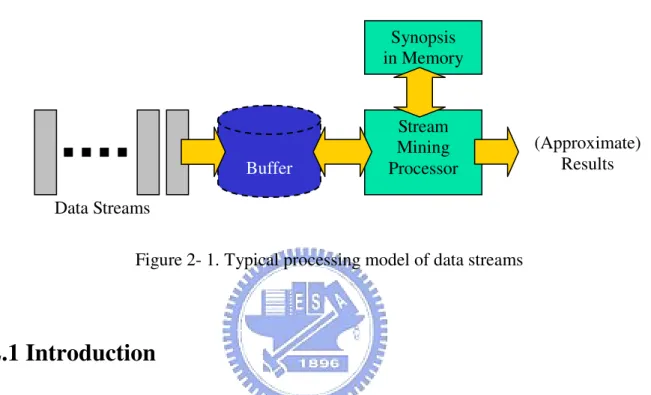
Online mining of data streams differs from traditional mining of static datasets in the following aspects [6]. First, each data element in streaming data should be examined at most once. Second, the memory usage for mining data streams should be bounded even though new data elements are continuously generated from the stream. Third, each data element in the stream should be processed as fast as possible. Fourth, the analytical results generated by the online mining algorithms should be instantly available when requested by the users. Finally, the frequency errors of outputs generated by the online algorithms should be as small as possible. The online processing model of data streams is shown in Figure 2-1.
As described above, the continuous nature of streaming data makes it essential to use the online algorithms which require only one scan over the data streams for knowledge discovery. The unbounded characteristic makes it impossible to store all the data into the main memory or even in secondary storage. This motivates the design of summary data structure with small
7
footprints that can support both one-time and continuous queries of streaming data. In other words, one-pass algorithms for mining data streams have to sacrifice the exactness of its analytical results by allowing some tolerable counting errors. Hence, traditional multiple-pass techniques studied for mining static datasets are not feasible to mine patterns over streaming data.
Figure 2- 1. Typical processing model of data streams
2.1 Introduction
Frequent itemsets mining is one of the most important research issues in data mining. The problem of frequent itemsets mining of static datasets (not streaming data) was first introduced by Agrawal et al. [2] described as follows. Let Ψ = {i1, i2, …, in} be a set of
literals, called items. Let database DB be a set of transactions, where each transaction T contains a set of items, such that T ⊆ Ψ. The size of database DB is the total number of transactions in DB and is denoted by |DB|. A set of items is referred to as an itemset. An itemset X with l items is denoted by X = (x1x2… xl), such that X ⊆ Ψ. The support of an
itemset X is the number of transactions in DB containing the itemset X as a subset, and denoted by sup(X). An itemset X is frequent if sup(X) ≥ minsup⋅|DB|, where minsup is a user-specified minimum support threshold in the range of [0, 1]. Consequently, given a database DB and a user-defined minimum support threshold minsup, the problem of mining
Stream Mining Processor Synopsis in Memory Buffer (Approximate) Results Data Streams
8
frequent itemsets in static datasets is to find the set of all itemsets whose support is no less than minsup⋅|DB|. In this paper, we will focus on the problem of mining frequent itemsets over the entire history of data streams.
Many previous studies contributed to the efficient mining of frequent itemsets in streaming data. According to the stream processing model [70], the research of mining frequent itemsets in data streams can be divided into three categories: landmark windows,
sliding windows, and damped windows, as described briefly as follows. In the landmark windows model, knowledge discovery is performed based on the values between a specific timestamp called landmark and the present time. In the sliding windows model, knowledge discovery is performed over a fixed number of recently generated data elements as the target of data mining. In the damped windows model, recent sliding windows are more important than previous ones.
In [53], Manku and Motmani developed two single-pass algorithms, Sticky-Sampling and Lossy Counting, to mine frequent items over a landmark window. Moreover, Manku and Motwani proposed the first single-pass algorithm BTS (Buffer-Trie-SetGen) based on the Lossy-Counting [53] to mine the set of frequent itemsets (FI) from streaming data. Chang and Lee [11] proposed a BTS-based algorithm for mining frequent itemsets in sliding windows model. Moreover, Chang and Lee [10] also developed another algorithm, called estDec, for mining frequent itemsets in streaming data in which each transaction has a weight decreasing with age. In other words, older transactions contribute less toward itemset frequencies, and it is a kind of damped windows model. Teng et al. [63] proposed a regression-based algorithm, called FTP-DS, to find frequent itemsets across multiple data streams in a sliding window. Lin
et al. [51] proposed an incremental mining algorithm to find the set of frequent itemsets in a time-sensitive sliding window. Giannella et al. [31] proposed a frequent pattern tree (abbreviated as FP-tree) [35] based algorithm, called FP-stream, to mine frequent itemsets at
9
multiple time granularities by a novel tilted-time windows technique. Yu et al. [68] discussed the issues of false negative or false positive in mining frequent itemsets from high speed transactional data streams. Jin and Agrawal [39] proposed an algorithm, called StreamMining, for in-core frequent itemset mining over data streams. Chi et al. [18] proposed an algorithm, called MOMENT, that might be the first to find frequent closed itemsets (FCI) from data streams. A summary data structure called CET is used in the MOMENT algorithm to maintain the information of closed frequent itemsets.
Because the focus of the chapter is on frequent itemses mining over data streams with a landmark window, we mainly address this issue by comparison with the BTS algorithm proposed by Manku and Motwani [53]. In the following, we describe the BTS algorithm in detail. In the BTS algorithm, two estimated parameters: minimum support threshold s, and
maximum support error threshold ε, are used, where 0 < ε ≤ s < 1. The incoming data stream is conceptually divided into buckets of width w = 1/ε transactions each, and the current length of the stream is denoted by N transactions.
The BTS algorithm is composed of three steps. In the first step, BTS repeatedly reads a
batch of buckets into main memory. In the second step, it decomposes each transaction within the current bucket into a set of itemsets, and stores these itemsets into a summary data structure D which contains a set of entries of the form (e, e.freq, e.∆), where e is an itemset,
e.freq is an approximate frequency of the itemset e, and e.∆ is the maximum possible error in
e.freq.
For each itemset e extracted from the incoming transaction T, BTS performs two operations to maintain the summary data structure D. First, it counts the occurrences of e in the current batch, and updates the value e.freq if the itemset e already exists in the structure D. Second, BTS creates a new entry (e, e.freq, e.∆) in D, if the itemset e does not occur in D, but its estimated frequency e.freq in the batch is greater than or equal to |batch|⋅ε, where the value
10
of maximal possible error e.∆ is set to |batch|⋅ε, and |batch| denotes the total number of transactions in the current batch. To bound the space requirement of D, BTS algorithm deletes the updated entry e if e.freq + e.∆ ≤ |batch|⋅ε. Finally, BTS outputs those entries ei in D, where
ei.freq ≥ (s−ε)⋅N, when a user requests a list of itemsets with the minimum support threshold s
and the support error threshold ε.
The motivation of the proposed work is to develop a method that utilizes some space-effective summary data structures to reduce the cost in mining frequent itemsets over data streams. In this paper an efficient, single-pass algorithm, referred to as Data Stream
Mining for Frequent Itemsets (abbreviated as DSM-FI), is proposed to improve the efficiency of frequent itemset mining in data streams. A new summary data structure called summary
frequent itemset forest (abbreviated as SFI-forest) is developed for online incremental maintaining of the essential information about the set of all frequent itemsets of data streams generated so far.
The proposed algorithm DSM-FI has three important features: a single pass of streaming data for counting the support of significant itemsets; an extended prefix tree-based, compact pattern representation of summary data structure; and an effective and efficient search and determination mechanism of frequent itemsets. Moreover, the frequency error guarantees provided by DSM-FI algorithm is the same as that of BTS algorithm. The error guarantees are stated as follows. First, all itemsets whose true support exceeds s⋅N are output. Second, no itemsets whose true support is less than (s − ε)⋅N is output. Finally, estimated supports of itemsets are less than the true support by at most ε⋅N.
The comprehensive experiments show that our algorithm is efficient on both sparse and dense data, and scalable to the continuous data streams. Furthermore, DSM-FI algorithm outperforms BTS, a state-of-the-art single-pass algorithm, by one order of magnitude for discovering the set of all frequent itemsets over the entire history of the data streams.
11
The remainder of the chapter is organized as follows. Section 2.2 defines the problem of single-pass mining frequent itemsets in a landmark window over data streams. The proposed DSM-FI algorithm is described in Section 2.3. The extended prefix tree-based summary data structure SFI-forest is introduced to maintain the essential information about the set of all frequent itemsets of the stream generated so far. Theoretical analysis and experiments are presented in Section 2.4. We conclude the chapter in Section 2.5.
2.2 Problem Definition
Based on the estimation mechanism of the BTS algorithm, we propose a new, single-pass algorithm to improve the efficiency of mining frequent itemsets over the entire history of data streams when a user-specified minimum support threshold s ∈ (0, 1), and a maximum support error threshold ε ∈ (0, s) are given.
Let Ψ = {i1, i2, …, im} be a set of literals, called items. An itemset is a nonempty set of
items. A l-itemset, denoted by (x1x2… xl), is an itemset with l items. A transaction T consists
of a unique transaction identifier (tid) and a set of items, and denoted by <tid, (x1x2… xq)>,
where xi ∈ Ψ, ∀i =1, 2, …, q. A basic window W consists of k transactions. The basic
windows are labeled with window identifier wid, starting from 1.
Definition 2-1 A data stream, DS = [W1, W2, …, WN), is an infinite sequence of basic
windows, where N is the window identifier of the “latest” basic window. The current length of DS, written as DS.CL, is k⋅N, i.e., |W1| + |W2| + … + |WN|. The windows arrive in some
order (implicitly by arrival time or explicitly by timestamp), and may be seen only once.
Mining frequent itemsets in landmark windows over data streams is to mine the set of all frequent itemsets from the transactions between a specified window identifier called landmark and the current window identifier N. Note that the value of landmark is set to 1.
12
To ensure the completeness of frequent itemsets for data streams, it is necessary to store not only the information related to frequent itemsets, but also the information related to infrequent ones. If the information about the currently infrequent itemsets were not stored, such information would be lost. If these itemsets become frequent later on, it would be impossible to figure out their correct support and their relationship with other itemsets. The data stream mining algorithms have to sacrifice the exactness of the analytical results by allowing some tolerable support errors since it is unrealistic to store all the streaming data into the limited main memory. Hence, we define two types of support of an itemset, and divide the itemsets embedded in the stream into three categories: frequent itemsets, significant itemsets, and infrequent itemsets.
Definition 2-2 The true support of an itemset X, denoted by X.tsup, is the number of
transactions in the data stream containing the itemset X as a subset. The estimated support of an itemset X, denoted by X.esup, is the estimated true support of X stored in the summary data structure, where 0 < X.esup ≤ X.tsup.
Definition 2-3 The current length (CL) of data stream with respect to an itemset X stored in
the summary data structure, denoted by X.CL, is (N−j+1)⋅k, i.e., |Wj| + |Wj+1| + … + |WN|,
where Wj is the first basic window with the window identifier j stored in the current summary
data structure containing the itemset X, and N is the window identifier of current window.
Definition 2-4 An itemset X is frequent if X.tsup ≥ s⋅X.CL. An itemset X is significant if s⋅X.CL > X.tsup ≥ ε⋅X.CL. An itemset X is infrequent if ε⋅X.CL > X.tsup.
Definition 2-5 A frequent itemset is maximal if it is not a subset of any other frequent
itemsets generated so far.
13
threshold s in the range of [0, 1], and a user-specified maximum support error threshold ε in the range of [0, s], the problem of mining frequent itemsets in landmark windows over data streams is to find the set of all frequent itemsets in single scan of the data stream.
2.3 The Proposed Algorithm: DSM-FI
The proposed DSM-FI (Data Stream Mining for Frequent Itemsets) algorithm consists of four steps.
(a) Read a basic window of transactions from the buffer in main memory, and sort
the items of transaction in the lexicographical order (Step 1).
(b) Construct and maintain the in-memory summary data structure (Step 2).
(c) Prune the infrequent information from the summary data structure (Step 3).
(d) Find the frequent itemsets from the summary data structure (Step 4).
Steps 1 and 2 are performed in sequence for a new incoming basic window. Step 3 is performed after every basic window has been processed. Finally, step 4 is usually performed periodically or when it is needed. Since the reading of a basic window of transactions from the buffer is straightforward, we shall henceforth focus on Steps 2, 3, and 4, and devise algorithms for effective construction and maintenance of summary data structure, and efficient determination of frequent itemsets.
2.3.1
Construction and Maintenance of Summary Data structure
In this section, we describe the algorithm which constructs and maintains the in-memory summary data structure called SFI-forest (Summary Frequent Itemset forest).
Definition 2-6 A summary frequent itemset forest (SFI-forest) is a summary data structure
14
1. SFI-forest consists of a frequent item list (FI-list), and a set of summary frequent
itemset trees (SFI-trees) of item-prefixes, denoted by item-prefix.SFI-trees.
2. Each node in the item-prefix.SFI-tree consists of four fields: item-id, item-id.esup,
item-id.window-id, and item-id.node-link. The first field item-id is the item identifier
of the inserting item. The second field item-id.esup registers the number of transactions represented by a portion of the path reaching the node with the item-id. The value of the third field item-id.window-id assigned to a new node is the window identifier of the current window. The final field item-id.node-link links up a node with the next node with the same item-id in the same SFI-tree or null if there is none. 3. Each entry in the FI-list consists of four fields: item-id, item-id.esup,
item-id.window-id, and item-id.head-link. The item-id registers which item identifier
the entry represents, item-id.esup records the number of transactions containing the item carrying the item-id, the value of item-id.window-id assigned to a new entry is the window identifier of current window, and item-id.head-link points to the root node of the item-id.SFI-tree. Note that each entry with item-id in the FI-list is an item-prefix and it is also the root node of the item-id.SFI-tree.
4. Each item-prefix.SFI-tree has a specific opposite frequent item list (OFI-list) with respect to the item-prefix, denoted by item-prefix.OFI-list. The item-prefix.OFI-list is
composed of four fields: item-id, item-id.esup, item-id.window-id, and
item-id.head-link. The item-prefix.OFI-list operates the same as the FI-list except that
the field head-link links to the first node with the same item-id in the
item-prefix.SFI-tree. Note that |item-prefix.OFI-list| = |FI-list| in the worst case, where |FI-list| denotes the total number of entries in the FI-list.
Figure 2-2 outlines the SFI-forest construction of the proposed DSM-FI algorithm. First of all, DSM-FI algorithm reads a transaction T from the current window BN. Then, DSM-FI
15
projects this transaction T into many sub-transactions, and inserts these sub-transactions into the SFI-forest. The details of this projection are described as follows. A transaction T with m items, such as (x1x2… xm), in the current window should be projected by inserting m
item-prefix sub-transactions into the SFI-forest. In other words, the transaction T = (x1x2… xm)
is converted into m sub-transactions; that is, (x1x2… xm), (x2x3… xm), …, (xm-1xm), and (xm).
These m sub-transactions are called item-prefix transactions, since the first item of each sub-transaction is an item-prefix of the original transaction T. This step, called transaction
projection, is denoted by TP(T) = {x1|T, x2|T, …, xi|T, …, xm|T}, where xi|T = (xixi+1… xm), ∀i
= 1, 2, …, m. The projecting cost of a transaction of length m for constructing the summary data structure SFI-forest is (m2+m)/2, i.e., m + (m−1) + … + 2 + 1. Recall that the decomposing cost of a transaction with m items of BTS algorithm for constructing the summary data structure is (2m−2). In general, the constructing cost of summary data structure of our algorithm is extremely less than that of BTS algorithm.
After performing the transaction projection of the incoming transaction T, DSM-FI algorithm inserts T into the FI-list, and then removes T from the current window in the main memory. Then, the items of these item-prefix transactions are inserted into the
item-prefixes.SFI-trees as branches, and the estimated support of the corresponding
item-prefixes.OFI-lists are updated. If an itemset shares a prefix of an itemset already in the SFI-tree, the new itemset will share a prefix of the branch representing that itemset. In addition, an estimated support counter is associated with each node in the tree. The counter is updated when an item-prefix transaction causes the insertion of a new branch. Figure 2-3 shows the subroutines of SFI-forest construction and maintenance.
Example 2-1. Let the Wj be a window with the landmark identifier j, and it contains six
transactions: < acdf >, < abe >, < df >, < cef >, < acdef > and < cef >, where a, b, c, d, e and f are items in the data stream. The SFI-forest with respect to the first two transactions, < acdf >
16
and < abe >, constructed by DSM-FI algorithm is described as follows. Note that each node of the form (id: id.esup: id.wid) is composed of three fields: item-id, estimated support, and
window-id. For example, (a: 2: j) indicates that, from basic window Wj to current basic
window WN (1 ≤ j ≤ N), item a appeared twice.
Algorithm SFI-forest construction
Input: A data stream, DS = [B1, B2, …, BN) with landmark 1, a user-specified minimum
support threshold s∈(0, 1), and a maximum support error threshold ε ∈ (0, s).
Output: A SFI-forest generated so far.
1: FI-list = {}; /*initialize the FI-list to empty.*/ 2: foreach window Bj do /* j = 1, 2, …, N */
3: foreach transaction T = (x1x2… xm) ∈ Bj (j = 1, 2, …, N) do
/* m ≥ 1 and j is the current window identifier */ 4: foreach item xi ∈ T do /* the maintenance of FI-list */
5: if xi ∉ FI-list then
6: create a new entry of form (xi, 1, j, head-link) into the FI-list;
/* the entry form is (item-id, item-id.esup, window-id, head-link)*/ 7: else /* the entry already exists in the FI-list*/
8: xi.esup = xi.esup + 1;
/* increment the estimated support of item-id xi by one*/
9: end if 10: end for 11: call TP(T, j);
/* project the transaction with each item-prefix xi for constructing the xi.SFI-tree */
12: end for
13: call SFI-forest-pruning(SFI-forest, ε, N); /* Step 3 of DSM-FI algorithm */ 14: end for
Figure 2- 2. Algorithm SFI-forest Construction
17
Input: A transaction T = (x1x2… xm) and the current window-id j;
Output: xi.SFI-tree, ∀i = 1, 2, …, m;
1: foreach item xi, ∀i = 1, 2, …, m, do
2: SFI-tree-maintenance([xi|X], xi.SFI-tree, j);
/* X = x1, x2, …, xm is the original incoming transaction T */
/* [xi|X] is an item-prefix transaction with the item-prefix xi*/
3: end for
Subroutine SFI-tree-maintenance /* Step 2 of DSM-FI algorithm */
Input: An item-prefix transaction (xixi+1… xm), the current window-id j, and xi.SFI-tree, where
i=1, 2, …, m;
Output: A modified xi.SFI-tree, where i=1, 2, ..., m;
1: foreach item xl do /* l = i+1, i+2, …, m */
2: if xl ∉ xi.OFI-list then /* xi.OFI-list maintenance */
3: create a new entry of form (xl, 1, j, head-link) into the xi.OFI-list;
/* the entry form is (item-id, item-id.esup, item-id.window-id,
item-id.head-link)*/
4: else /* the entry already exists in the xi.OFI-list */
5: xl.esup = xl.esup + 1;
/* increment the estimated support of item-id xl by one*/
6: end if 7: endfor
8: foreach item xi, ∀i = 1, 2, …, m, do /* xi.SFI-tree maintenance */
9: if SFI-tree has a child node with item-id y such that y.item-id = xi.item-id then
10: y.esup = y.esup +1; /*increment y’s estimated support by one*/ 11: else create a new node of the form (xi, 1, j, node-link);
/* initialize the estimated support of the new node to one, and link its parent link to SFI-tree, and its node-link linked to the nodes with same item-id via the node-link structure. */
12: end if 13: end for
18
Subroutine SFI-forest-pruning /* Step 3 of DSM-FI algorithm: prune the infrequent
information from the SFI-forest */
Input: A SFI-forest, a user-specified maximum support error threshold ε, and the current
window identifier N;
Output: A SFI-forest which contains the set of all significant and frequent itemsets.
1: foreach entry xi (i=1, 2, …, d) ∈ FI-list, where d =|FI-list| do
2: if xi .esup < ε⋅⋅⋅⋅xi.CL then /* if xi is an infrequent item */
3: delete xi.SFI-tree;
4: delete the entry xi from the FI-list;
5: delete xi from other xj.OFI-list if it exists in xj.OFI-list (j = 1, 2, …, d; j ≠ i);
6: delete those nodes (item-id = xi) in other SFI-trees via node-link structures and
merge the fragmented sub-trees;
/* a simple way is to reinsert or to join the remainder sub-trees into the SFI-tree */; 7: end if
8: end for
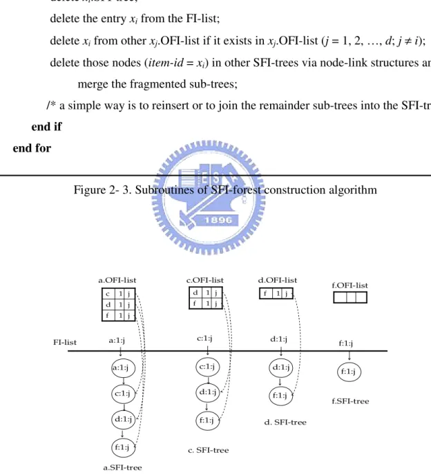
Figure 2- 3. Subroutines of SFI-forest construction algorithm
a:1:j c:1:j f:1:j d:1:j c:1:j f:1:j d:1:j f:1:j d:1:j f:1:j a:1:j c:1:j d:1:j f:1:j a.SFI-tree c. SFI-tree d. SFI-tree f.SFI-tree a.OFI-list f.OFI-list d.OFI-list c.OFI-list FI-list j 1 f j 1 d j 1 c j 1 f j 1 d f 1 j
19 a:2:j c:1:j f:1:j d:1:j c:1:j f:1:j d:1:j f:1:j d:1:j f:1:j e:1:j a:2:j c:1:j d:1:j f:1:j e:1:j a.SFI-tree c.SFI-tree d.SFI-tree e.SFI-tree f.SFI-tree a.OFI-list f.OFI-list e.OFI-list d.OFI-list c.OFI-list FI-list j 1 b j 1 e j 1 f j 1 d j 1 c j 1 f j 1 d f 1 j b:1:j e:1:j b:1:j b.SFI-tree j 1 e b.OFI-list b:1:j e:1:j
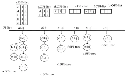
Figure 2- 5. SFI-forest construction after processing the second transaction < abe >
(a) First transaction < acdf >: First of all, DSM-FI algorithm reads the first transaction and calls the Transaction-Projection(< acdf >). Then, DSM-FI inserts four item-prefix transactions: <acdf>, <cdf>, <df>, and <f> into the FI-list, [a.SFI-tree, a.OFI-list], [c.SFI-tree, c.OFI-list], [d.SFI-tree, d.OFI-list], and [f.SFI-tree, f.OFI-list], respectively. The result is shown in Figure 2-4. In the following steps, the head-links of each
item-prefix.OFI-list are omitted for concise presentation.
(b) Second transaction <abe>: DSM-FI algorithm reads the second transaction and calls the Transaction-Projection(<abe>). Next, DSM-FI inserts three item-prefix transactions: <abe>, <be>, and <e> into the FI-list, [a.SFI-tree, a.OFI-list], [b.SFI-tree, b.OFI-list], and [e.SFI-tree, e.OFI-list], respectively. The result is shown in Figure 2-5. After processing all the transactions of window Wj, the SFI-forest generated so far is shown in Figure 2-6.
2.3.2
Pruning Infrequent Information from SFI-forest
According to the Apriori principle, only the frequent 1-itemsets are used to construct candidate k-itemsets, where k ≥ 2. Thus, the set of candidate itemsets containing the
20
infrequent items stored in the summary data structure is pruned. The pruning is usually performed periodically or when it is needed.
Let the maximum support error threshold be ε in the range of [0, s], where s is a user-defined minimum support threshold in the range of [0, 1]. The space pruning method of DSM-FI is that the item x and its supersets are deleted from SFI-forest if x.esup < ε⋅x.CL. For each entry (x, x.esup, x.window-id, x.head-link) in the FI-list, if its x.esup is less than ε⋅x.CL, it can be regarded as an infrequent item. In this case, three operations are performed in sequence. First, DSM-FI deletes the x.OFI-list, x.SFI-tree, and the infrequent entry x from the FI-list. Second, DSM-FI removes the infrequent item x of other OFI-lists by traversing the FI-list. Third, DSM-FI deletes the infrequent item x from other SFI-trees, and reconstructs these SFI-trees. After pruning all infrequent items from SFI-forest, SFI-forest contains the set of all frequent itemsets and significant itemsets of the data stream generated so far.
a:3:j c:2:j e:1:j d:2:j f:1:j c:4:j e:1:j d:2:j f:1:j e:1:j d:3:j f:1:j f:5:j e:4:j f:3:j a:3:j c:4:j d:3:j f:5:j e:4:j a.SFI-tree c.SFI-tree d.SFI-tree e.SFI-tree f.SFI-tree f.OFI-list e.OFI-list d.OFI-list c.OFI-list FI-list j 1 b j 2 e j 2 f j 2 d j 2 c j 3 e j 4 f j 2 d j 1 e j 3 f j 3 f b:1:j e:1:j b:1:j b.SFI-tree j 1 e b.OFI-list b:1:j e:1:j e:2:j f:2:j f:1:j f:1:j f:2:j a.OFI-list
21 a:3:j c:2:j e:1:j d:2:j f:1:j c:4:j e:1:j d:2:j f:1:j e:1:j d:3:j f:1:j f:5:j e:4:j f:3:j a:3:j c:4:j d:3:j f:5:j e:4:j a.SFI-tree c.SFI-tree d.SFI-tree e.SFI-tree f.SFI-tree
a.OFI-list c.OFI-list d.OFI-list f.OFI-list e.OFI-list
FI-list j 2 f j 2 e j 2 d j 2 c j 4 f j 3 e j 2 d j 3 f j 1 e f 3 j e:1:j e:2:j f:2:j f:1:j f:1:j f:2:j
Figure 2- 7. SFI-forest after pruning all infrequent items
Example 2-2: Let the maximum support error threshold ε be 0.2. Hence, an itemset X is infrequent in Figure 2-6 if X.esup < ε⋅X.CL. Note that ε⋅X.CL = 0.2⋅6 = 1.2. After computing the current window Wj, the next step of DSM-FI is to prune all the infrequent items from the
current SFI-forest. At this time, DSM-FI deletes the b.SFI-tree, b.OFI-list, and item b itself from the FI-list, since item b is an infrequent item; that is, b.esup = 1 < 1.2. Then, DSM-FI updates the a.OFI-list and reconstructs a.SFI-tree, because a.OFI-list and a.SFI-tree contains the infrequent item b. The result is shown in Figure 2-7.
The next step of DSM-FI is to determine the set of all frequent itemsets from SFI-forest constructed so far. The step is performed only when the current results of the data stream is requested. Note that the number of candidate 2-itemsets is a performance bottleneck in the Apriori-based frequent itemset mining algorithms [3, 35]. DSM-FI algorithm can avoid this performance problem. This is because DSM-FI can generate all frequent 2-itemsets immediately by combining the frequent items in the FI-list with the frequent items in the corresponding OFI-list.
22
2.3.3
Determining Frequent Itemsets from Current SFI-forest
Once SFI-forest containing all the frequent items of the data stream generated so far is constructed, we can derive all the frequent itemsets by traversing the SFI-forest according to the Apriori principle. Therefore, we propose an efficient mechanism called top-down frequent
itemset selection (todoFIS), as shown in Figure 2-8, for mining frequent itemsets. It is especially useful in mining long frequent itemsets. The method is described as follows.
Assume that there are k frequent items, namely e1, e2, …, ek, in the current FI-list, and
each item ei, ∀i = 1, 2, …, k, has an associated ei.OFI-list, where the size of ei.OFI-list is
denoted by |ei.OFI-list|. Note that the items, namely o1, o2, …, oj, within the ei.OFI-list are
denoted by ei.o1, ei.o2, …, ei.oj, respectively, where the value j equals to |ei.OFI-list|. For each
entry ei, ∀i = 1, 2, …, k, in the current FI-list, DSM-FI algorithm first generates a maximal
candidate itemset with (j+1) items, i.e., (eiei.o1ei.o2 …ei.oj) by combining the item-prefix ei
with all frequent items in ei.OFI-list. Then, DSM-FI uses the following scheme to count its
estimated support.
First, we start with a specific frequent item ei.ol (1 ≤ l ≤ j), whose estimated support is
smallest, and traverse the paths containing ei.ol via node-links of ei.SFI-tree to count the
estimated support of the candidate (eiei.o1ei.o2 …ei.oj). If the estimated support of the
candidate is greater than or equal to (s−ε)⋅ ei.CL, then it is a frequent itemset. All subsets of
this frequent itemset are also frequent itemsets according to the Apriori principle. Hence, the complete set of the frequent itemsets stored in the ei.SFI-tree can be generated by enumeration
of all the combinations of the subsets of frequent (j+1)-itemset, (eiei.o1ei.o2 …ei.oj). On the
other hand, if the estimated support of the candidate (j+1)-itemset is less than the threshold (s−ε)⋅ ei.CL, then it is not a frequent itemset. Now, we need to use the same mechanism to test
all the subsets of the (j+1)-itemset until the candidate 3-itemsets. This is because all frequent 2-itemsets can be generated by combining the item ei and the frequent items of the ei.OFI-list.
23
Note that a (j+1)-itemset can be decomposed into C(j+1, j) j-itemsets. We decompose one candidate j-itemset from the (j+1)-itemset at a time, and use the same scheme described above to count the estimated support of this candidate j-itemset. Finally, all the maximal frequent itemsets are maintained in a temporal MFI-list, called MFItemp-list, for efficient generation of
the set of all frequent itemsets. If such a MFItemp-list is obtained, all the frequent itemsets can
be generated efficiently by enumerating the set of all maximal frequent itemsets in the current MFItemp-list without any candidate generation and support counting. Note that if the user
request is just to find the set of all maximal frequent itemsets so far, DSM-FI algorithm can output all maximal frequent itemsets efficiently by scanning the MFItemp-list.
Example 2-3. Let the minimum support threshold s be 0.5. Therefore, an itemset X is frequent
in Figure 2-7 if X.esup ≥ s⋅X.CL. Note that s⋅X.CL = 0.5⋅6 = 3 in this case. The online mining steps of DSM-FI algorithm are described as follows.
(1) First of all, DSM-FI starts the frequent itemset mining scheme from the first frequent item
a (from left to right). At this moment, only item a is a frequent itemset, since the estimated support of items c, d, e, and f in the a.OFI-list are less than s⋅a.CL, where s⋅a.CL = 3. Now, DSM-FI stores the maximal frequent 1-itemset (a) into the MFItemp-list.
(2) Next, DSM-FI starts on the second entry c for frequent itemset mining. DSM-FI generates a candidate maximal 3-itemset (cef), and traverses the c.SFI-tree to count its estimated support. As a result, the candidate (cef) is a maximal frequent itemset, since its estimated support is 3 and it is not a subset of any other frequent itemsets in the MFItemp-list. Now,
DSM-FI stores the maximal frequent itemset (cef) into the MFItemp-list.
(3) Next, DSM-FI starts on the third entry d and generates a candidate maximal 2-itemset (df). DSM-FI stores the itemset (df) into the MFItemp-list without traversing d.SFI-tree because
(df) is a frequent 2-itemset and is not a subset of any other maximal frequent itemsets stored in the MFItemp-list.
24
(4) On the fourth entry f, DSM-FI algorithm generates one frequent 1-itemset (f) directly, since the f.OFI-list is empty. DSM-FI does not store it into the MFItemp-list, because (f) is a
subset of a generated maximal frequent itemset (cef).
Finally, on the fifth entry e, DSM-FI generates a frequent 2-itemset (ef) directly. However, the frequent 2-itemset (ef) is a subset of a maximal frequent itemset (cef) stored in the MFItemp-list.
DSM-FI algorithm does not store it into the MFItemp-list.
Algorithm todoFIS
Input: A current SFI-forest, the current window identifier N, a minimum support threshold s,
and a maximum support error threshold ε.
Output: A set of all frequent itemsets.
1: MFItemp-list = ∅;
/* MFItemp-list is a temporary list used to store the set of maximal frequent itemsets */
2: foreach entry e in the current FI-list do
3: construct a maximal candidate itemset E with size |E| /* |E| = 1+|e.OFI-list| */ 4: count E.esup by traversing the e.SFI-tree;
5: if E.esup ≥ (s−ε) ⋅⋅⋅⋅E.CL then
6: if E ⊄ MFItemp-list and E is not a subset of any other patterns in the
MFItemp-list
then
7: add E into the MFItemp-list;
8: remove E’s subsets from the MFItemp-list;
9: end if
10: else /* if E is not a frequent itemset */
11: enumerate E into itemsets with size |E|−1; 12: end if
13: until todoFIS finds the set of all frequent itemsets with respect to entry e; 14: end for
25
After processing all the entries in the FI-list, the MFItemp-list generated by DSM-FI
algorithm contains the set of current maximal frequent iemsets: {(a), (cef), (df)}. Therefore, the set of all frequent itemsets can be generated by enumerating the set: {(a), (cef), (df)}. Consequently, the set of all frequent itemsets in Figure 2-7 are {(a), (cef), (ce), (cf), (ef), (c), (e), (f), (df), (d)}.
2.4 Theoretical Analysis
In this section, we discuss the upper bound of estimated support error of frequent itemsets generated by DSM-FI algorithm, and the space upper bound of prefix-tree-based summary data structure.
2.4.1
Maximum Estimated Support Error Analysis
In this section, we discuss the maximum estimated support error of all frequent itemsets generated by DSM-FI algorithm. Let X.wid be the window-id of itemset X stored in the current SFI-forest. Assume that the window contains k transactions. Let the maximum support error threshold be ε. Let the current window-id of the incoming stream be wid(N). Now, we have the following theorem of maximum estimated support error guarantee of frequent itemsets generated by the proposed algorithm.
Theorem 2-1 X.tsup − X.esup ≤ ε⋅(X.wid −1)⋅k.
Proof: We prove by induction. Base case (X.wid = 1): X.tsup = X.esup. Thus, X.tsup − X.esup
≤ ε⋅(X.wid −1)⋅k.
Induction step: Consider an itemset of the form (X, X.esup, X.wid) that gets deleted for some wid(N) > 1. The itemset is inserted in the SFI-forest when wid(N+1) is being processed. The itemset X whose window-id is wid(N+1) in the FI-list could possibly have been deleted as