國 立 交 通 大 學
電信工程研究所
碩 士 論 文
在 HCCA 架構下是否使用負載式運送
To Piggyback or Not to Piggyback in HCCA
研究生:劉永祥
在 HCCA 架構下是否使用負載式運送
To Piggyback or Not to Piggyback in HCCA
研 究 生:劉永祥 Student:Yung-Hsiang Liu
指導教授:李程輝 Advisor:Tsern-Huei Lee
國 立 交 通 大 學
電信工程研究所
碩 士 論 文
A ThesisSubmitted to Institute of Communication Engineering College of Electrical and Computer Engineering
National Chiao Tung University in partial Fulfillment of the Requirements
for the Degree of Master
in
Communication Engineering June 2010
Hsinchu, Taiwan, Republic of China
在 HCCA 架構下是否使用負載式運送
學生:劉永祥
指導教授
:李程輝 教授
國立交通大學電信工程研究所碩士班
摘
要
負載式運送(piggyback)能有效的減少 MAC 層的在協定上耗費的時間. 然而,
它並不是所有情況皆適用. 在某些情況下, 它會受到”重傳”與”負載式運送問題”
的影響而減少頻帶使用的效能. 針對資料(data)訊框,確認(Ack)訊框與免競爭輪詢
( C F - p o l l ) 訊框有多種負載式運送的方式 . 為了追求最高的效能, 我們想找
出不同情況下最佳的作法.
首先, 我們只專注在資料訊框與確認訊框是否需要合併運送的問題上.接著討
論在 HCCA 的架構下, 是否需要將免競爭輪詢訊框也一起合併的問題. 在考慮有
位元錯誤率與不同的傳輸速率的情況下, 我們分別計算各種情況的平均有效傳
送量(throughput)來選出最好的方式傳送. 根據我們研究發現,在某些情況下這種
做法可以改善高達 50% 的效能.
To Piggyback or Not to Piggyback in HCCA
student:Yung-Hsiang Liu
Advisors:Dr. Tsern-Huei Lee
Institute of Communication Engineering
National Chiao Tung University
ABSTRACT
Piggyback is an effective way to reduce the MAC protocol overhead. However, it
is not always useful in every environment. In some cases, it may decrease the channel
efficiency due to the retransmissions and the piggyback problem. There are some rules
to piggyback with data frame, ack frame and CF-poll frame. In order to maximize the
throughput, we have to find out which way has the best efficiency. First, we focus
only on piggybacking data and Ack frame or not. Second, we also discuss the CF-poll
frame in HCCA. Considering the transmission bit error and transmission rate, we
estimate the average throughput then choose a way to transmit. The improvement of
piggyback can reach 50% in some case.
誌
謝
經過兩年來的研究所生活,時間過的很快也很充實,雖然在研究過程中難免
遇到一些挫折,但是總能找出方法克服。能夠順利完成這篇論文,要感謝的人太
多了。首先感謝我的指導老師 – 李程輝教授。感謝這段時間以來對我的指導與
照顧,以及讓我有公開發表與參與校內外研討的機會。感謝郭耀文教授,在每次
開會討論時總能提出重要的建議,給予我們很多很好的研究方向。感謝同實驗室
的郁文學長、景融學長、啟賢學長,還有不同實驗室的柏宇,在我遇到無法解決
的問題時陪我討論尋找答案。感謝所有實驗室裡的成員,讓我這兩年的研究所生
活充滿了歡笑。
當然更要感謝我的父親 – 劉福龍先生,母親 – 黃珀玲女士,以及家人對我
的關心,在他們的全力支持下,我才能專注於我的研究上。還有我的女朋友秀秀,
雖然唸的是不同領域,但仍能在許多挫折中互相扶持。感謝大家~
謹將此論文獻給身邊所有愛我的人及我愛的人
2010 新竹交大
目
錄
中文提要
... i
英文提要
... ii
誌謝
... iii
目錄
... iv
表目錄
... v
圖目錄
... vi
Chapter 1
Introduction... 1
Chapter 2
System Model... 3
2.1
To piggyback Ack with data frame or not... 3
2.2
To piggyback or not in HCCA... 4
Chapter 3
Mathematical Analysis... 6
3.1
To piggyback Ack with data frame or not... 6
3.1.1 No
piggyback
Case... 7
3.1.2
Piggyback Case... 8
3.2
To piggyback or not in HCCA... 10
Chapter 4
Numerical Results... 15
4.1
To piggyback Ack with data frame or not... 15
4.2
To piggyback or not in HCCA... 18
Chapter 5
Conclusion... 21
Reference ... 22
表目錄
Table 1-
Valid type and subtype combinations... 2
Table 2- The notations used for 3.1... 6
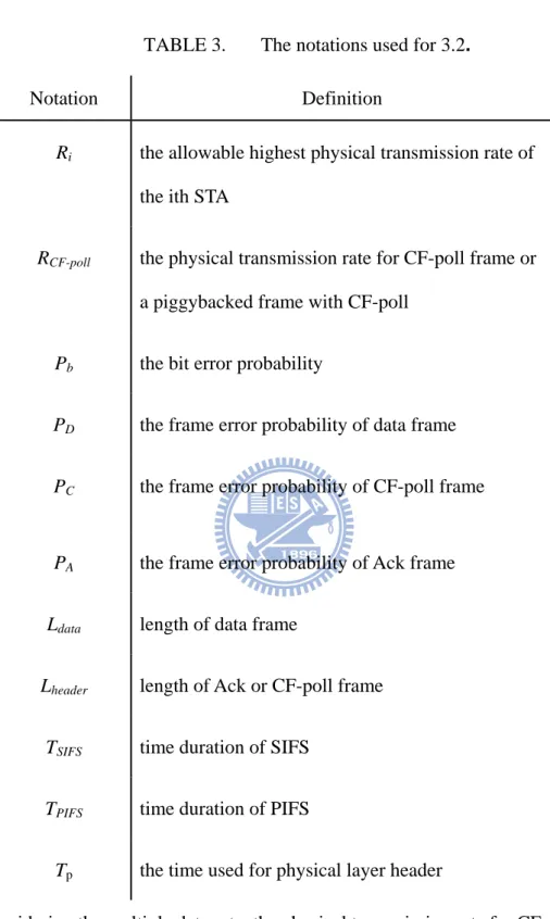
Table 3- The notations used for 3.2... 10
圖目錄
Figure 1. “To piggyback Ack or not” scenario...4
Figure 2. The scenario in contention-free period...4
Figure 3. Two cases for computing F
p... 9
Figure 4. Two cases for computing G
i,I...9
Figure 5. The case 1 scheme...11
Figure 6. The case 2 scheme...12
Figure 7. The case 3 scheme...13
Figure 8. The case 4 scheme...14
Figure 9. Throughput comparison for R
d=12Mbps and P
b=10
-5...16
Figure 10. Throughput comparison for R
d=54Mbps and P
b=10
-5...16
Figure 11. Throughput comparison for R
d=54Mbps and P
b=10
-4...17
Figure 12. Throughput comparison for R
d=36Mbps and P
b=10
-5...17
Figure 13. Throughput comparison for R1=6, R2=9, R3=12, R4=18, R5=24, R6=24,
R7=54, R8=54, R9=54, R10=54Mbps and the Pb=10
-4...18
Figure 14. Throughput comparison for Ri =54Mbps, i = 1~10 and Pb= 10
-6...19
Figure 15. Throughput comparison for R1=24, Ri =54Mbps, i = 2~10 and Pb= 10
-6...19
Chapter 1
Introduction
IEEE 802.11 wireless LAN is used for a long time and accepted for different environment with many generations such as 11a, 11b, 11g, etc. In 802.11a/g, it provides eight different transmission rates from 6Mbps to 54Mbps by different modulation and coding. In order to maximizing the throughput, RBAR (receiver based auto rate) and ARF (auto rate fallback) are used for choosing a proper transmission rate. In RBAR, the receiver has to estimate the channel quality and feedback to the transmitter and the transmitter can adapt for the next time. But in ARF, the STA increases the transmission rate after ten consecutive successful transmissions and decreases after two consecutive retransmissions without the channel information sending from the receiver.
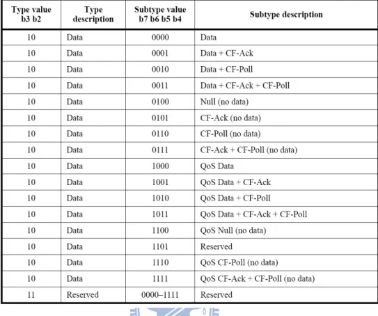
IEEE 802.11e HCF controlled channel access (HCCA) supports the reservation-based QoS, and provides many combination rules for the different types of frames. (table 1) Such as a CF-poll frame is used to allow a station (STA) to use the wireless channel and set the network allocation vector (NAV) for the other stations. An acknowledgement (Ack) frame is sent to the transmitter which transmitted the previous data frame by the receiver when the data frame is received successfully. These two frames can be piggybacked in a data frame to reduce the MAC overhead and increase the channel efficiency because the piggyback only needs to modify the header but not increases the length of data frame. The wireless station can perform piggyback according to the table 1 and no complex computation is required.
TABLE 1. Valid type and subtype combinations.
However, in some cases, it may decrease the channel efficiency due to the retransmissions [1] and the piggyback problem [2]. If an Ack frame which is piggybacked in a data frame failed to be received, the previous data frame needs to be retransmitted again although it was received successfully. A CF-poll frame and a data frame which is piggybacked with CF-poll should be transmitted in the minimum transmission rate of the allowable rate for all STAs to make sure that all STAs can receive the CF-poll and set their NAV. In [2], the author defined the piggyback problem as : The channel efficiency is decreased when the CF-poll frame is piggybacked in the data frame when any STA has the low physical transmission rate.
In this paper, we divide into two parts. First, we focus only on piggybacking Ack with data frame or not. Second, we also discuss the CF-poll frame. We want to maximize the throughput and choose the best way to transmit Ack, data, and CF-poll frames for the transmitter by evaluating the cost of time and efficiency for all cases.
C
HAPTER2
System Model
To improve the throughput, the transceiver will use the best achievable rate for the data frames. Because of the uncertainty of wireless communication, this is an error-prone environment such that frames may be corrupted during the transmission. We assume that the system has error detection code for detecting the corrupted frames.
2.1 To piggyback Ack with data frame or not
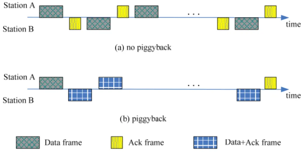
We consider a pair of wireless network, say station A and B. They have frames to each other and transmit frames as shown in figure 1(a). The minimum interval between two successive frames is the short inter frame space (SIFS). If the STA which transmitted the data frame does not receive the Ack frame from the receiver STA within a timeout interval, it will retransmit the same data frame again in its next round. The timeout interval is PCF inter frame space (PIFS).
For an Ack frame sent by a receiver, it is usually transmitted at the basic rate such that the bit error rate is extremely low. Therefore, in this case, the error probability of Ack frames is assumed to be negligible.
The Ack frame can be also piggybacked with data frame as shown in figure 1(b). If this is an error-free environment, the efficiency increases in this way. However, it may also decreases in some cases. In error-prone environment, it is possible fail to transmit or receive the “data+Ack” frame and the frame has to be retransmitted again.
Figure 1. “To piggyback Ack or not” scenario.
2.2 To piggyback or not in HCCA
We consider a wireless network. There are one access point (AP) and n STAs.
The AP has one data frame to each STA, and polls every STA in sequence. The STAs also have one data frame to AP during their Transmission Opportunity (TXOP). Besides, they will s e n d a n A c k b a c k i f n e c e s s a r y. We a s s u m e t h a t t h e l e n g t h o f d a t a frames and the bit error rate are fixed. The scheme shows in figure 2.
In figure 2, there are piggybacked frames “Ack + data + CF-poll” from STA2 to STAn. In order to find out how to piggyback this frame or not that can maximize the throughput, we divided into four cases 1 , 2 , 3 and 4.
In case 1, the piggybacked frame “Ack , data , CF-poll” will be transmitted individually. In case 2 and 3, we separate it into two frames “Ack + data, CF-poll” and “Ack, data +CF-poll”. And in case 4, we just piggyback together but not separate it. But there is no “Ack + CF-poll, data”. If the AP polled the next STA before it transmitted the data frame, there will be a collision. There is no “data, Ack + CF-poll”, too. Because after AP transmitted the data frame, the Ack will be time-out and the previous data frame will be retransmitted again in the next TXOP. In this four cases, if a STA did not receive the CF-poll or CF-poll in a piggybacked data frame successfully, then the AP should poll again after PIFS. The other intervals between two frames are defined as SIFS.
Chapter 3
Mathematical Analysis
3.1 To piggyback Ack with data frame or not
In order to discussing the “piggyback Ack or not” issue, the queue length at both STAs must be equal. We assume that there are i equal-length frames in each queue of STAs. The notations used in this part are listed as follows.
TABLE 2. The notations used for 3.1.
Notation Definition
R the basic physical rate used for Ack frames
Rd the physical rate used for data frames
Pb the bit error probability with physical rate Rd
P the frame error probability of data frame
TSIFS time duration of SIFS
TPIFS time duration of PIFS
L length of data frame
La length of Ack frame
Tp the time used for physical layer header
Td the time spent when a data frame is successfully
transmitted
Ta the time spent to transmit an Ack frame
Ta= Tp+8 ×La/R+TSIFS
Tr the time spent when a data frame is corrupted
Tr= Tp+8 ×L/Rd+TSIFS+TS
Fx the average time spent to successfully transmit the
considered data frames to their destination under a specific operation. Fn and Fp are for the normal case
and the piggyback case respectively.
3.1.1 No piggyback case
In this case, each frame is transmitted separately. A STA needs to retransmit the data frame if the Ack frame is not received. Let M be the random variable representing the number of retransmission times before a data frame is successfully transmitted. The probability mass function can be calculated by
(
)
i(1
),
p M
= =
i
P
× −
P
(1) which is a geometric distribution with mean M equal to P/(1-P).Therefore, the time used to successfully transmit a data frame can be calculated by
.
r d
T
=
M
×
T
+
T
(2)3.1.2 Piggyback case
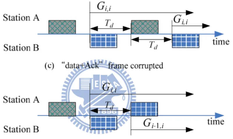
We assume that there are i data frames at station A and j frames at station B when a station receives a data or a “data+Ack” frame successfully. Let Gi,j be the average time spent
to service (i+j) frames. After the first data frame is transmitted, there are two cases for the destined station as shown in figure 3(a) and 3(b). If the frame is corrupted, the whole process restarts. On the other hand, the data frame is received successfully, and the time spent to deliver the rest frames is equal to Gi,i. Therefore, we have
,
(
) (1
)
.
p d s p i i
F
=
T
+ ×
P
T
+
F
+ −
P
×
G
(5)If it is corrupted as shown in figure 4(c), the source station will retransmit again and the time required is equal to Td+ Gi,i. As shown in figure 4(d), the time required is equal to Gi-1,i .
,
(
,) (1
)
1,.
i i d d i i i iG
=
T
+ ×
P
T
+
G
+ −
P
×
G
− (6) 1,(
1,)
(1
)
1, 1,
i i d d i i i iG
−=
T
+ ×
P
T
+
G
−+ −
P
×
G
− − (7) 1,1 d(
d 1,1) (1
)
0,1,
G
=
T
+ ×
P
T
+
G
+ −
P
×
G
(8) 0,1 a.
G
=
T
(9) ,1
(2
1)
,
1
i i d aP
G
i
T
T
P
+
= × −
×
+
−
(10)(2
2
)
,
1
d s p ai
i P
P T
PT
F
T
P
× + × × −
+
=
+
−
(11) 2 8 (1 ) Throughupt lim 8. (1 ) i p d i L P L F P T →∞ × × × − ≈ = × × + × (12) ․․․Figure 3. Two cases for computing Fp.
Figure 4. Two cases for computing Gi,i.
The frame error probability P can be computed by 8
1 (1
b)
L.
3.2 To piggyback or not in HCCA
TABLE 3. The notations used for 3.2.
Notation Definition
Ri the allowable highest physical transmission rate of
the ith STA
RCF-poll the physical transmission rate for CF-poll frame or
a piggybacked frame with CF-poll
Pb the bit error probability
PD the frame error probability of data frame
PC the frame error probability of CF-poll frame
PA the frame error probability of Ack frame
Ldata length of data frame
Lheader length of Ack or CF-poll frame
TSIFS time duration of SIFS
TPIFS time duration of PIFS
Tp the time used for physical layer header
Considering the multiple data rate, the physical transmission rate for CF-poll frame or a piggybacked frame with CF-poll is
CF.Poll 1
R
= min{ }
ii n
R
≤ ≤ , (14) where the n means the number of STAs.
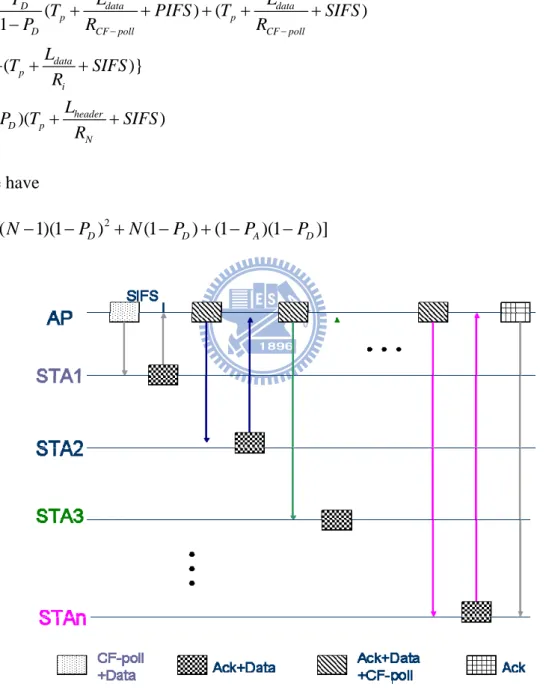
Case 1.
In case 1, the frames will be transmitted separately. The scheme shows in figure 5. The cost of time in case 1, T can be calculated by 1
(15) And we have the average bits successfully transmitted P 1
(16) 1 1 1 [ ( ) ( )] ( ) 1 {[(1 )( )] 0 ( ) [(1 )( )] 0 ( ) ( 1
data data data
D
p p p
D CF poll CF poll
header data header
D p D p D p D i i i C header p p C CF poll L L L P
T T PIFS T SIFS T SIFS
P R R R
L L L
P T SIFS P T SIFS P T SIFS P
R R R P L T PIFS T P R − − − − = + + + + + + + + − − + + + × + + + + − + + + × + + + + + + − 2 ) ( )} (1 )( ) N i header data p CF poll i header D p N L L SIFS T SIFS R R L P T SIFS R = − + + + + + − + +
∑
1[(1
D)(1
A)(2
1) (1
D)]
P
=
L
−
P
−
P
N
− + −
P
2
2 [(1 D)(1 A) (1 D) (1 D) ( 1)]
P =L −P −P N+ −P + −P N −
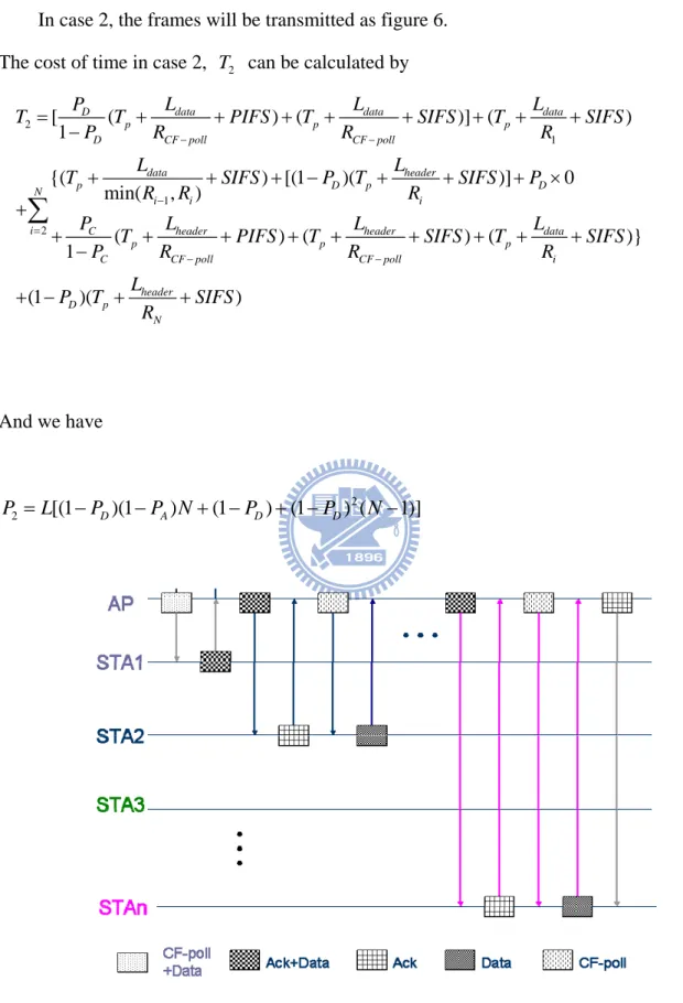
Case 2.
In case 2, the frames will be transmitted as figure 6. The cost of time in case 2, T can be calculated by 2
(17)
And we have
(18)
Figure 6. The case 2 scheme.
2 1 1 [ ( ) ( )] ( ) 1 {( ) [(1 )( )] 0 min( , ) ( ) ( ) ( 1
data data data
D p p p D CF poll CF poll data header p D p D i i i C header header p p p C CF poll CF poll L L L P
T T PIFS T SIFS T SIFS
P R R R L L T SIFS P T SIFS P R R R P L L T PIFS T SIFS T P R R − − − − − = + + + + + + + + − + + + − + + + × + + + + + + + + − 2 )} (1 )( ) N i data i header D p N L SIFS R L P T SIFS R = + + + − + +
∑
Case 3.
In case 2, the frames will be transmitted as figure 7. The cost of time in case 3, T can be calculated by 3
(19) And we have (20) 3 1 1 2 [ ( ) ( )] ( ) 1 {[(1 )( )] 0 ( ) ( ) ( )} 1 (1 )(
data data data
D p p p D CF poll CF poll header D p D N i
i D data data data
p p p
D CF poll CF poll i
D p
L L L
P
T T PIFS T SIFS T SIFS
P R R R L P T SIFS P R L L L P
T PIFS T SIFS T SIFS
P R R R P T − − − = − − = + + + + + + + + − − + + + × + + + + + + + + + + − + −
∑
) header N L SIFS R + + 3 [(1 D)(1 A) (1 D) ] P =L −P −P N+ −P NCase 4.
In case 4, the frames will be transmitted as figure 8. The cost of time in case 4, T can be calculated by 4
(21) And we have
(22)
Figure 8. The case 4 scheme.
4 1 2 [ ( ) ( )] ( ) 1 { ( ) ( ) 1 ( )} (1 )( )
data data data
D p p p D CF poll CF poll data data D p p N D CF poll CF poll i data p i header D p N L L L P
T T PIFS T SIFS T SIFS
P R R R L L P T PIFS T SIFS P R R L T SIFS R L P T SIFS R − − − − = = + + + + + + + + − + + + + + − + + + + + − + +
∑
2 4 [( 1)(1 D) (1 D) (1 A)(1 D)] P =L N− −P +N −P + −P −PChapter 4
Numerical Results
In this section, we present some numerical results about the benefit of piggyback. We use different bit error rate and the data rate to calculate the throughput for each case. In figure 9~16, the horizontal axis means the length of data frames and the vertical axis is the average throughput. We calculate the average throughput for different bit-error-rate and the transmission rates of STAs.
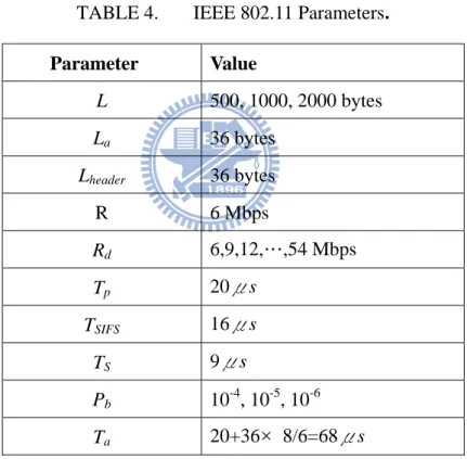
The parameters used in this section are listed in table 4. TABLE 4. IEEE 802.11 Parameters.
Parameter Value L 500, 1000, 2000 bytes La 36 bytes Lheader 36 bytes R 6 Mbps Rd 6,9,12,…,54 Mbps Tp 20μs TSIFS 16μs TS 9μs Pb 10-4, 10-5, 10-6 Ta 20+36 × 8/6=68μs
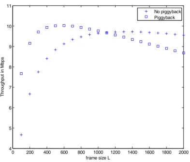
0 200 400 600 800 1000 1200 1400 1600 1800 2000 4 5 6 7 8 9 10 11 frame size L Th ro ughp ut in M bp s No piggyback Piggyback
Figure 9. Throughput comparison for Rd=12Mbps and Pb=10-5.
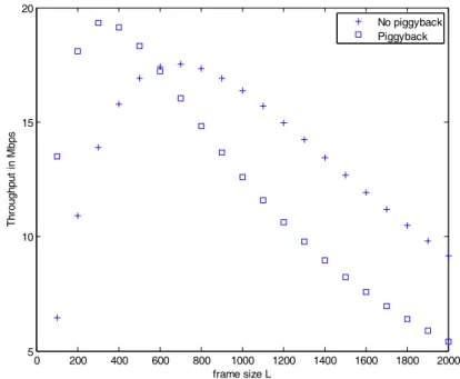
Figure 10 shows the results for 54Mbps under the same bit error rate. The crossover point moves to over 2000 bytes. That is, it is better to piggyback all the time for high data rate because the time wasted in retransmitting the “data+Ack” frames is reduced. The throughput improvement by piggyback in the best case is about 40%.
0 200 400 600 800 1000 1200 1400 1600 1800 2000 5 10 15 20 25 30 35 40 frame size L Th ro ughp ut in M bp s No piggyback Piggyback up 40%
Figure 10. Throughput comparison for Rd=54Mbps and Pb=10-5.
Figure 11 shows the results for Rd=54Mbps and Pb=10-4. With larger bit error rate, the
throughput decreases due to lots of retransmission, especially for large data frames.
0 200 400 600 800 1000 1200 1400 1600 1800 2000 5 10 15 20 frame size L T hr oughpu t i n M bps No piggyback Piggyback
Figure 11. Throughput comparison for Rd=54Mbps and Pb=10-4.
Assume that we can have Pb=10-5 with Rd =36Mbps. The results are plotted in Figure 12.
It is interesting to check what happens if the bit error rate is reduced. We can see that the throughput is over 20Mbps for most cases. Therefore, one should trade off between bit error rate and physical data rate to achieve best performance. The way to perform link adaptation affects the effective throughput.
15 20 25 30 oughput in Mbps
4.2 To piggyback or not in HCCA
With the formulas we derived in previous section3.2 the effect of piggyback in four cases can be evaluated in terms of the average throughput.
Figure 13 shows the throughput in four cases for R1=6, R2=9, R3=12, R4=18, R5=24,
R6=24, R7=54, R8=54, R9=54, R10=54Mbps and the Pb=10-5. We can see that the line for case
1 is better than the others all the time, which means the AP should not piggyback. The improvement of piggyback can reach 50% in this case. Besides, the throughput is very low for the short length of data frames.
Figure 13. Throughput comparison for R1=6, R2=9, R3=12, R4=18, R5=24, R6=24, R7=54,
Figure 14 shows the result for Ri =54Mbps, i = 1~10 and Pb= 10-6. The case 4 gets the
lead and the case 1 is the worst now. The AP should piggyback the Ack and CF-poll in the data frame because there are not so many disadvantages of piggyback such as retransmission or “piggyback CF-poll” problem.
Figure 14. Throughput comparison for Ri =54Mbps, i = 1~10 and Pb= 10-6.
Figure 15 shows the result for R1=24, Ri =54Mbps, i = 2~10 and Pb= 10-6.
Figure 16 shows the result for Ri =54Mbps, i = 1~10 and Pb= 2*10-5.
The case 3 is the best about 1100-1500 bytes.
Figure 16. Throughput comparison for Ri =54Mbps, i = 1~10 and Pb= 2*10-5.
In summary, piggyback is not always the best choice to transmit this frame. Under some conditions, the best way is to transmit all separately or use two frames “Ack + data, CF-poll” and “Ack, data +CF-poll”.
If the bit-error-rate is large and the RCF-poll is low, it is definitely better not to use
piggyback for avoiding the excessive retransmissions and “piggyback CF-poll” problem. On the contrary, if the bit-error-rate is small and all the transmission rate of STAs are high enough, the AP should piggyback the Ack and CF-poll in the data frame to increase the throughput.
When the bit-error-rate is small and the RCF-poll is low but not too low, the case 2 will get
the lead. We should mind the RCF-poll here. If it is too low, the throughput of case 2 will
decrease and be worse than case 1 because the slowest STA slow down the total transmission rate. If it is too high, the throughput of case 2 will be worse than case 4 for the reason above.
We can hardly find out a condition that the case 3 is the best. Only when the RCF-poll is
high and the bit-error-rate is large but not too large, the case 3 is the best. If the bit-error-rate is too large, the CF-poll piggybacked in data frame suffers from too many retransmissions so the case 3 is worse than case 1. If too small, the case 3 is worse than case 4.
Chapter 5
Conclusions
In some case, we can use piggyback to improve our system efficiency and the improvement of piggyback can reach 50%. However, piggyback is not always effective in
every environment. Sometimes we should transmit separately instead of piggybacking. Moreover, the length of data frame has a great effect on the frame error rate. In principle, when the bit-error-rate is high, the length should choose not too large in order to decreasing retransmissions. But when the bit-error-rate is low, using a small frame has a worse throughput because of the effect of protocol overhead. With the influence of transmission rate, the length of data frames also can be chosen by the formulas to have a better throughput. However, we just bring up the principle to remind the effect of length. We don’t maximize the throughput by choosing the best length of data frame, because the length of data frame isn’t only determined by AP or STAs but also determined by arrival-rate, type of data(ex: video, voice ). The tradeoff between data rate and bit error is still an open issue and we will also focus on it.
Reference
[1] T. H. Lee, Y. W. Kuo, Y. W. Hung, and Y. H. Liu, “To Piggyback Or Not to Piggyback Acknowledgement?” , in Proc. IEEE VTC’10, pp. 76-87990, May. 2010.
[2] H. J. Lee, J. H. Kim, and S. Cho, “A Novel Piggyback Selection Scheme in IEEE 802.11e HCCA”, in Proc. IEEE ICC’07, pp. 4529-4534, Jun. 2007.
[3] IEEE Standard for Information technology-Telecommunications and information exchange between systems-Local and metropolitan area networks-Specific requirements – “Part 11: Wireless LAN Medium Access Control (MAC) and Physical Layer (PHY) Specifications,” 2007.
[4] IEEE Draft Standard for Information Technology-Telecommunications and information exchange between systems--Local and metropolitan area networks--Specific requirements – “Part 11: Wireless LAN Medium Access Control (MAC) and Physical Layer (PHY) specifications Amendment 5: Enhancements for Higher Throughput,” Mar. 2009.
[5] G. Holland, N. Vaidya, and P. Bahl, “A Rate-Adaptive MAC Protocol for Multi-hop Wireless Networks,” in Proc. of MOBICOM 2001, Rome, Italy, Jul., 2001, 236-251. [6] A. Kamerman and L. Montean, “WaveLan-II: A High-Performance Wireless LAN for
the Unlicensed Band,” Bell Labs Technical Journal, pp.118-133, Summer, 1997. [7] Y. Xiao, “IEEE 802.11 performance enhancement via concatenation and piggyback
mechanisms,” IEEE Trans. on Wireless Commun., vol. 4, no.5, pp. 2182-2192, Sep. 2005.