An Efficient Algorithm for Mining Frequent Itemests
over the Entire History of Data Streams
Hua-Fu Li1, Suh-Yin Lee1 and Man-Kwan Shan2 1
Department of Computer Science and Information Engineering, National Chiao-Tung University, No. 1001 Ta Hsueh Road, Hsinchu, Taiwan 300, R.O.C.
{hfli, sylee}@csie.nctu.edu.tw
2
Department of Computer Science, National Chengchi University, No. 64, Sec. 2, Zhi-nan Road, Wenshan, Taipei, Taiwan 116, R.O.C.
Abstract. A data stream is a continuous, huge, fast changing, rapid, infinite sequence of data elements. The nature of streaming data makes it essential to use online algorithms which require only one scan over the data for knowledge discovery. In this paper, we propose a new single-pass algorithm, called DSM-FI (Data Stream Mining for Frequent Itemsets), to mine all frequent itemsets over the entire history of data streams. DSM-FI has three major features, namely single streaming data scan for counting itemsets’ frequency information, extended prefix-tree-based compact pattern representation, and top-down frequent itemset discovery scheme. Our performance study shows that DSM-FI outperforms the well-known algorithm Lossy Counting in the same streaming environment.
1 Introduction
Mining frequent itemsets is an essential step in many data mining problems, such as mining association rules, sequential patterns, closed patterns, maximal pattern, and many other important data mining tasks. The problem of mining frequent itemsets in large databases was first proposed by Agrawal et al. [2] in 1993, and the problem can be defined as follows. Let Ψ = {i1, i2, …, in} be a set of literals, called items. Let database DB be a set
of transactions, where each transaction T consists of a set of items, such that T ⊆ Ψ. Each
transaction is also associated with a unique transaction identifier, called TID. A set X ⊆ Ψ
is also called an itemset, where items within an itemset are kept in lexicographic order. A
k-itemset is represented by (x1, x2, …, xk), where x1 < x2 < …< xk. The support of an
itemset X, denoted sup(X), is the number of transactions in which that itemset occurs as a subset. An itemset X is called a frequent itemset if sup(X) ≥ ms*|DB|, where ms ∈ (0, 1) is a user-specified minimum support threshold and |DB| is the size of the database. Hence, the problem of mining frequent itemsets is to mine all itemsets whose support is no less than ms*|DB| in a large database.
Recently, database and data mining communities have focused on a new data model, where data arrives in the form of continuous streams. It is often referred to data streams or
streaming data. Many applications generate large amount of data streams in real time,
Web record and click streams in Web applications, performance measurement in network monitoring and traffic management, call records in telecommunications, etc. Mining such streaming data differs from traditional data mining in following aspects [3]: First, each data element in streaming data should be examined at most once. Second, memory usage for mining data streams should be bounded even though new data elements are continuously generated from the data stream. Third, each data element in data streams should be processed as fast as possible. Fourth, the results generated by the online algorithms should be instantly available when user requested. Finally, the frequency errors of the outputs generated by the online algorithms should be constricted as small as possible. Hence, the nature of streaming data makes it essential to use online algorithms which require only one scan over the data for knowledge discovery. Moreover, it is not possible to store all the data in main memory or even in secondary storage. This motivates the design for in-memory summary data structure with small memory footprints that can support both one-time and continuous queries. In other words, data stream mining algorithms have to sacrifice the correctness of its analysis result by allowing some
counting errors. Consequently, previous multiple-pass data mining techniques studied for
traditional datasets cannot be easily solved for the streaming data domain.
In this paper, we discuss the problem of mining frequent itemsets in data streams [8, 6, 9, 4, 5]. According to the data stream processing model [10], the research of mining frequent itemsets in data streams can be divided into three fields: landmark windows model [8],
sliding windows model [9,5], and damped windows model [6, 4], as described briefly as
follows. The first scholars to give much attention to mining all frequent itemsets over the entire history of the streaming data were Manku and Motwani [8]. The proposed algorithm Lossy Counting is a first single-pass algorithm based on a well-known Apriori-property [2]: if any length k pattern is not frequent in the database, it length (k+1) super-patterns
can never be frequent. Lossy Counting uses a specific array-representation to represent the
lexicographic ordering of the hash tree, which is the popular method for candidate counting [2]. Teng et al. [9] proposed a regression-based algorithm, called FTP-DS, to find frequent itemsets in sliding windows. Chang and Lee [4] develop an algorithm estDec for mining frequent itemsets in streaming data in which each transaction has a weight and it decrease with age. In other words, older transactions contribute less toward itemset frequencies. Moreover, Chang and Lee [5] also proposed a single-pass algorithm for mining recently frequent itemsets based on the estimation mechanism of the algorithm Lossy Counting. Giannella et al. [6] developed a tree-based algorithm [7], called FP-stream, to mine frequent itemsets at multiple time granularities by a novel titled-time windows technique.
In this paper, we present an efficient algorithm DSM-FI for mining all frequent itemsets by one scan of the streaming data. DSM-FI has three major features, namely single streaming data scan for counting itemsets’ frequency information, extended prefix-tree-based compact pattern representation, and top-down frequent itemset discovery scheme. The experiments show that DSM-FI is efficient on both sparse and dense data streams. Furthermore, DSM-FI outperforms the well-known algorithm Lossy Counting for mining all frequent itemsets over the entire history of the data streams.
2 Problem Definition
Based on the estimation mechanism of the Lossy Counting algorithm [8], we propose a new single-pass algorithm for mining all frequent itemsets in data streams based on a
landmark windows model when a user-specified minimum support threshold ms ∈ (0, 1),
and a user-defined maximal estimated support error threshold ε ∈ (0, ms) are given. For
mining all frequent itemsets, a data stream can be defined as follows.
Let Ψ = {i1, i2, …, im} be a set of literals, called items. Let data stream DS = B1, B2, …,
BN, …, be an infinite sequence of blocks, where each block is associated with a block
identifier i, and N is the identifier of the “latest” block BN. Each block Bi consists of a
timestamp tsi, and a set of transactions; that is, Bi =[tsi, T1, T2, …, Tk], where k ≥ 0. Hence,
the current length (CL) of the data stream is defined as CL = |B1|+|B2|+…+|BN|. A
transaction T consists of a set of items, such that T ⊆ Ψ. Moreover, each transaction is
also associated with a unique transaction identifier, called TID. A set of items X is also
called an itemset and an itemset X with k items is denoted as (x1x2…xk), such that X ⊆ Ψ.
Due to the unique characteristics of streaming data, any one-pass algorithms have to sacrifice the correctness of their analysis results by allowing some errors. Hence, the True
support of an itemset X, denoted by Tsup(X), is the number of transactions seen so far in
which that itemsets occurs as a subset, and the Estimated support of the itemset X, denoted as Esup(X), is the estimated true support of X stored in the summary data structure constructed by the one-scan approaches, where Esup(X) ≤ Tsup(X). An itemset X is called
a frequent itemset if Tsup(X) ≥ ms*CL. An itemset is called a sub-frequent itemset if
ms*CL > Tsup(X) ≥ ε * CL. Furthermore, an itemset is called an infrequent itemset if ε*CL
> Tsup(X). An itemset is called a maximal frequent itemset if it is not a subset of any other frequent itemsets generated so far.
Hence, given a user-defined minimum support threshold ms ∈ (0, 1), a user-specified
maximal estimated support error threshold ε ∈ (0, ms) and a data stream DS, our goal is to
develop a single-pass algorithm to mine all frequent itemsets in the landmark windows model of the streaming data using as little main memory as possible.
3
Algorithm DSM-FI
Algorithm DSM-FI is composed of four steps: reading a block of transactions (step 1), constructing the summary data structure (step 2), pruning the infrequent information from the summary data structure (step 3), and top-down frequent itemset discovery scheme (step 4). Step 1 and step 2 are performed in sequence for a new block. Step 3 and step 4 are usually performed periodically or when it is needed.
3.1 Efficient Mining Frequent Itemsets in Data Streams by DSM-FI
First of all, we define an in-memory summary data structure called IsFI-forest, and describe the construction of ISFI-forest. Then we use a running example to explore it.
Definition 1: An Item-suffix Frequent Itemset forest (or IsFI-forest in short) is an
extended prefix-tree-based summary data structure defined bellow.
1. IsFI-forest consists of a Dynamic Header Table (or DHT in short) and a set of
Candidate Frequent Itemset trees of item-suffixes (or CFI-trees(item-suffixes)in
short).
2. Each entry in the DHT consists of four fields: item-id, support, block-id, and
head-link, where item-id registers the identifier of item, support records the number of
transactions containing the item carrying the item-id, the value of block-id assigned to a new entry is the identifier of current block, and head-link points to the root node of
the CFI-tree(item-id). Notice that each entry e, for example, of DHT is an item-suffix and it is also the root node of the CFI-tree(e).
3. Each node in the CFI-tree(item-suffix) consists of four fields: item-id, support,
block-id, and node-link, where item-id is the identifier of the inserting item, support
registers the number of transactions represented by a portion of the path reaching the node with item-id, the value of block-id assigned to a new node is the identifier of current block, and node-link links to the next node carrying the same item-id in the IsFI-forest. If no such node, the node-link is null.
4. Each CFI-tree(item-suffix) has a specific Dynamic Header Table with respect to the
item-suffix (denoted as DHT(item-suffix)); moreover, the DHT(item-suffix) is
composed of four fields, namely item-id, support, block-id, and head-link. The DHT(item-suffix) operates the same as DHT except that node-link links to the first node carrying the item-id in the CFI-tree(item-suffix). Notice that |DHT(item-suffix)| = |DHT| in worst case, where |DHT| denotes the total number of entries in the DHT. The construction of IsFI-forest is described as follows. First of all, algorithm DSM-FI reads a transaction T from the current block. Then, DSM-FI projects this transaction into small transactions and inserts these transactions into DHT and IsFI-forest. In details, each
transaction, such as T = (x1x2…xk), in the current block BN is projected into the IsFI-forest
by inserting k item-suffix transactions in it. In other words, transaction T is converted into
k small transactions; that is, (x1x2x3…xk), (x2x3…xk), …, (xk-1xk) and (xk). In this paper, these
small transactions are called item-suffix transactions, since the first item in each transaction is an item-suffix of original transaction T. We called this step Item-suffix
Projection, and denoted it as IsProjection(T) = {x1|T, x2|T, …, xk|T}, where x1|T =
(x1x2…xk), x2|T = (x2x3…xk), …, xk-1|T = (xk-1xk), xk|T = (xk)}, and T = (x1x2…xk). Algorithm
DSM-FI drop the original transaction T after IsProjection(T). Next, the set of items in these item-suffix transactions are inserted into these CFI-trees(item-suffixes) as a branch and updates these DHT(item-suffixes) according to the item-suffixes. If an itemset (i.e., item-suffix transaction) share a prefix with an itemset already in the tree, the new itemset will share a prefix of the branch representing that itemset. In addition, a support counter is associated with each node in the tree. The counter is updated when the next item-suffix transaction causes the insertion of a new branch. After pruning all infrequent information from the DHT, CFI-tree(item-suffix) and its corresponding DHT(item-suffix), and those CFI-trees containing this item-suffix, current IsFI-forest contains all essential information about all frequent itemsets of the stream seen so far. Let us examine an example as follows.
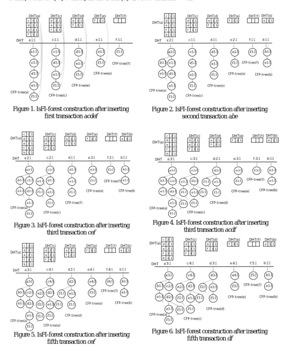
Example 1. Let the first block B1 of the data stream DS be (acdef), (abe), (cef), (acdf),
(cef), (df), the second block B2 be (def), (bef), (be), ms = 30%, and ε = 25%, where a, b, c,
d, e, f are items in the stream. Hence, there are six transactions in B1, and four transactions
in B2. Algorithm DSM-FI constructs the IsFI-forest with respect to the incoming block,
and prunes all infrequent information from the current IsFI-forest in the following steps.
Step 1. DSM-FI reads first block into main memory for constructing the IsFI-forest.
(a) First transaction acdef: First of all, DSM-FI reads the first transaction acdef and calls the IsProjection(acdef). Then, DSM-FI inserts these item-suffix transactions, acdef,
cdef, def, ef and f, into DHT, tree(a), DHT(a)], tree(c), DHT(c)],
[CFI-tree(d), DHT(d)], [CFI-tree(e), DHT(e)] and [CFI-tree(f), DHT(f)] respectively. The result is shown in Figure 1. In the following steps, from Figure 2 to Figure 6, we omit the head-links of each DHT(item-suffix) for concise representation.
(b) Second transaction abe: First, DSM-FI reads the second transaction abe and calls the
IsProjection(abe). Next, DSM-FI inserts these item-suffix transactions abe, be and e
into DHT, [CFI-tree(a), DHT(a)], [CFI-tree(b), DHT(b)] and [CFI-tree(e), DHT(e)] respectively. The result is shown in Figure 2.
(c) Third transaction cef: DSM-FI reads the third transaction cef and calls the
IsProjection(cef). Afterward, DSM-FI inserts the item-suffix transactions cef, ef and f
into DHT, [CFI-tree(c), DHT(c)], [CFI-tree(e), DHT(e)] and [CFI-tree(f), DHT(f)] respectively. The result is shown in Figure 3.
(d) Fourth transaction acdf: DSM-FI reads the fourth transaction acdf and calls the
IsProjection(acdf). Then, DSM-FI inserts these item-suffix transactions acdf, cdf, df
and f into DHT, [CFI-tree(a), DHT(a)], [CFI-tree(c), DHT(c)], [CFI-tree(d), DHT(d)] and [CFI-tree(f), DHT(f)] respectively. The result is shown in Figure 4.
(e) Fifth transaction cef: At this time, DSM-FI reads the fifth transaction cef and calls the
IsProjection(cef). Then, DSM-FI inserts the item-suffix transactions cef, ef and f into
DHT, [CFI-tree(c), DHT(c)], [CFI-tree(e), DHT(e)] and [CFI-tree(f), DHT(f)] respectively. The result is shown in Figure 5.
(f) Sixth transaction df: At this time, DSM-FI reads the sixth transaction df and calls the
IsProjection(df). Then, DSM-FI inserts the item-suffix transactions df and f into DHT,
[CFI-tree(d), DHT(d)] and [CFI-tree(f), DHT(f)] respectively. The result is shown in Figure 6.
Step 2. DSM-FI prunes all infrequent itemsets from the current IsFI-forest after processing
the first block B1. At this time, DSM-FI deletes the CFI-tree(b) and its corresponding
DHT(b), and prunes the entry b from the DHT, since item b is an infrequent item; that is,
Esup(b) < ε * CL. Then DSM-FI reconstructs the CFI-tree(a) by eliminating the
information about item b. The result is shown in Figure 7.
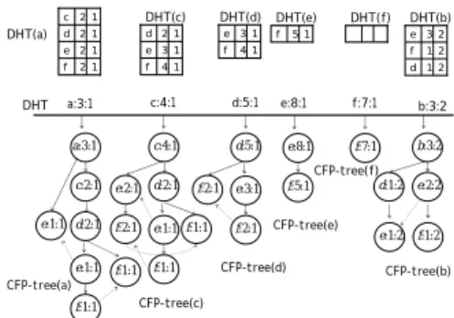
Step 3. DSM-FI reads second block into main memory for constructing the IsFI-forest.
The construction process of IsFI-forest with respect to block B2 is the same as Step 1 and
Step2. The result is shown in Figure 8.
The description, as stated above, is the construction process of IsFI-forest with respect to two incoming blocks over a continuous stream of transactions. From this process, we can see that one needs exactly one streaming data scan. Now, let us consider the frequent itemset discovery principle of DSM-FI discussed below.
First of all, given an item i (from left to right) in the current DHT, DSM-FI generates candidates by a “top-down” approach for minimum enumerating the combination of frequent itemsets within the item range of DHT(i). Then DSM-FI checks these candidates whether they are frequent ones or not by traversing the CFI-tree(i). The CFI-tree traversing principle is described as follows. First, DSM-FI generates a candidate maximal frequent itemset, k+1-itemset, containing all items within the DHT(i) (assume that |DHT(i)| = k). Second, DSM-FI traverses the CFI-tree via the node-links of the frequent item whose support is minimal for counting the estimated support of the maximal candidate. After that if the candidate is not a frequent itemset, DSM-FI generates some sub-candidates with k items. Next, DSM-FI executes the same CFI-tree traversing for
itemset counting, until it finds that these sub-candidates, j-itemsets where j ≥ 3, are
frequent ones. Notice that we can find the set of frequent 2-itemsets by combining the item-suffix i with the frequent items within the DHT(i).
Example 2. Let us mine the frequent itemsets from the current IsFI-forest in Figure 8. Let
ms be 0.3; that is, minimum support threshold of frequent itemsets from B1 to B2 is 3, but
in B2 is only 1.2. Now, we start the top-down frequent itemset discovery scheme from
frequent item a. At this moment, the frequent itemset is only (a), since the support of items, such as c, d, e and f, in the DHT(a) are less than ms * CL.
a:1:1 c:1:1 e:1:1 d:1:1 f:1:1 c:1:1 e:1:1 d:1:1 f:1:1 e:1:1 d:1:1 f:1:1 f:1:1 e:1:1 f:1:1 a:1:1 c:1:1 d:1:1 e:1:1 f:1:1 CFP-tree(a) CFP-tree(c) CFP-tree(e) CFP-tree(e) CFP-tree(f) DHT(a) DHT(c) DHT(d) DHT(e) DHT(f) DHT 1 1 f 1 1 e 1 1 d 1 1 c 1 1 f 1 1 e 1 1 d 1 1 f 1 1 e f 11
Figure 1. IsFI-forest construction after inserting first transaction acdef
a:2:1 c:1:1 e:1:1 d:1:1 f:1:1 c:2:1 e:1:1 d:1:1 f:1:1 e:1:1 d:1:1 f:1:1 f:2:1 e:3:1 f:2:1 a:2:1 c:2:1 d:1:1 e:3:1 f:2:1 CFP-tree(a) CFP-tree(c) CFP-tree(f) CFP-tree(e) CFP-tree(f) DHT(f) DHT(e) DHT(d) DHT(c) DHT 1 1 f 1 1 b 1 2 e 1 1 d 1 1 c 1 2 f 1 2 e 1 1 d 1 1 f 1 1 e f 21 b:1:1 e:1:1 b:1:1 CFP-tree(b) 1 1 e DHT(b) b:1:1 e:1:1 e:1:1 f:1:1 DHT(a)
Figure 3. IsFI-forest construction after inserting third transaction cef
a:3:1 c:2:1 e:1:1 d:2:1 f:1:1 c:4:1 e:1:1 d:2:1 f:1:1 e:1:1 d:2:1 f:1:1 f:4:1 e:4:1 f:3:1 a:3:1 c:4:1 d:2:1 e:4:1 f:4:1 CFP-tree(a) CFP-tree(e) CfP-tree(d) CFP-tree(e) CFP-tree(f) DHT(a) DHT(f) DHT(e) DHT(d) DHT(c) DHT 1 2 f 1 1 b 1 2 e 1 2 d 1 2 c 1 4 f 1 3 e 1 2 d 1 2 f 1 1 e f 31 b:1:1 e:1:1 b:1:1 CFP-tree(b) 1 1 e DHT(b) b:1:1 e:1:1 e:2:1 f:2:1 f:1:1 f:1:1 f:1:1
Figure 5. IsFI-forest construction after inserting fifth transaction cef
a:2:1 c:1:1 e:1:1 d:1:1 f:1:1 c:1:1 e:1:1 d:1:1 f:1:1 e:1:1 d:1:1 f:1:1 f:1:1 e:2:1 f:1:1 a:2:1 c:1:1 d:1:1 e:2:1 f:1:1 CFP-tree(a) CFP-tree(c) CFP-tree(e) CFP-tree(e) CFP-tree(f) DHT(a) DHT(f) DHT(e) DHT(d) DHT(c) DHT 1 1 f 1 1 b 1 2 e 1 1 d 1 1 c 1 1 f 1 1 e 1 1 d 1 1 f 1 1 e f 11 b:1:1 e:1:1 b:1:1 CFP-tree(b) 1 1 e DHT(b) b:1:1 e:1:1
Figure 2. IsFI-forest construction after inserting second transaction abe
a:3:1 c:2:1 e:1:1 d:2:1 f:1:1 c:3:1 e:1:1 d:2:1 f:1:1 e:1:1 d:2:1 f:1:1 f:3:1 e:3:1 f:2:1 a:3:1 c:3:1 d:2:1 e:3:1 f:3:1 CFP-tree(a) CFP-tree(c) CFP-tree(d) CFP-tree(e) CFP-tree(f) DHT(a) DHT(f) DHT(e) DHT(d) DHT(c) DHT 1 2 f 1 1 b 1 2 e 1 2 d 1 2 c 1 3 f 1 2 e 1 2 d 1 2 f 1 1 e f 21 b:1:1 e:1:1 b:1:1 CFP-tree(b) 1 1 e DHT(b) b:1:1 e:1:1 e:1:1 f:1:1 f:1:1 f:1:1 f:1:1
Figure 4. IsFI-forest construction after inserting third transaction acdf
a:3:1 c:2:1 e:1:1 d:2:1 f:1:1 c:4:1 e:1:1 d:2:1 f:1:1 e:1:1 d:3:1 f:1:1 f:5:1 e:4:1 f:3:1 a:3:1 c:4:1 d:3:1 e:4:1 f:5:1 CFP-tree(a) CFP-tree(c) CFP-tree(d) CFP-tree(e) CFP-tree(f) DHT(f) DHT(e) DHT(d) DHT(c) DHT 1 2 f 1 1 b 1 2 e 1 2 d 1 2 c 1 4 f 1 3 e 1 2 d 1 3 f 1 1 e f 31 b:1:1 e:1:1 b:1:1 CFP-tree(b) 1 1 e DHT(b) b:1:1 e:1:1 e:2:1 f:2:1 f:1:1 f:1:1 f:2:1 DHT(a)
Figure 6. IsFI-forest construction after inserting fifth transaction df
a:3:1 c:2:1 e:1:1 d:2:1 f:1:1 c:4:1 e:1:1 d:2:1 f:1:1 e:1:1 d:3:1 f:1:1 f:5:1 e:4:1 f:3:1 a:3:1 c:4:1 d:3:1 e:4:1 f:5:1 CFP-tree(a) CFP-tree(c) CFP-tree(d) CFP-tree(e) CFP-tree(f) DHT(a) DHT(f) DHT(e) DHT(d) DHT(c) DHT 1 2 f 1 2 e 1 2 d 1 2 c 1 4 f 1 3 e 1 2 d 1 3 f 1 1 e f 31 e:1:1 e:2:1 f:2:1 f:1:1 f:1:1 f:2:1
Figure 7. Current IsFI-forest after pruning any infrequent information with respect to infrequent
item b a:3:1 c:2:1 e:1:1 d:2:1 f:1:1 c:4:1 e:1:1 d:2:1 f:1:1 e:3:1 d:5:1 f:2:1 f:7:1 e:8:1 f:5:1 a:3:1 c:4:1 d:5:1 e:8:1 f:7:1 CFP-tree(a) CFP-tree(c) CFP-tree(d) CFP-tree(e) CFP-tree(f) DHT(a) DHT(f) DHT(e) DHT(d) DHT(c) DHT 1 2 f 1 2 e 1 2 d 1 2 c 1 4 f 1 3 e 1 2 d 1 4 f 1 3 e f 51 e:1:1 e:2:1 f:2:1 f:1:1 f:1:1 f:2:1 b:3:2 e:2:2 b:3:2 CFP-tree(b) f:1:2 d:1:2 e:1:2 DHT(b) 2 1 d 2 1 f 2 3 e
Figure 8. IsFI-forest construction after inserting the second incoming block B2 = {def, bef, bde, be}
Next, we start the top-down frequent itemset discovery scheme on the frequent item c. DSM-FI generates a candidate maximal 3-itemset (cef), and traverses the CFI-tree(c) for counting its support. At a result, the candidate (cef) is a (maximal) frequent itemset, since its support is 3. Now, DSM-FI generates frequent itemsets {(c), (e), (f), (ce), (cf), (ef), (cef)} directly based on the frequent itemset (cef), and stores the maximal frequent itemset (cef) in memory for further performance improvement.
Moreover, we start on the frequent item d, and generate a candidate maximal 3-itemset (def). By traversing the CFI-tree(d) using e’s node-link, we find that the candidate (def) is not a frequent itemset, since its support is 2. Then we directly generate two frequent 2-itemsets, (de) and (df), based on the DHT(d). At this moment, DSM-FI generates three frequent itemsets {(d), (de), (df)} in CFI-tree(d).
Furthermore, on item e and f, since their candidate maximal itemsets are subsets of previous maximal frequent itemset cef, we do not start the top-down frequent itemset mining process. This is because these frequent itemsets are already found by DSM-FI in previous phases.
Finally, we start the top-down frequent itemset mining on item b. DSM-FI directly generates a maximal frequent itemset (be), since be is a 2-itemset in CFI-tree(b).
3.2 Upper Bound of Space Requirement for Mining Data Streams
For a given DHT generated by DSM-FI, let the number of frequent items in the DHT be k.
Therefore, we know there are at most C⎣ ⎦k 2k/ maximal frequent itemsets in the data stream
seen so far. If we construct an IsFI-forest for all these maximal frequent itemsets, the tree
has height ⎣k/2⎦. In the first level, there are C⎣ ⎦/21
1 + k
nodes, in the second level, there are
C⎣ ⎦/2 2 2
+
k nodes, in the i-th level, there are C⎣ ⎦k i
i + 2
/ nodes, and in the last level, the ⎣k/2⎦ level,
there are C⎣ ⎦k 2k/ nodes. Thus, the total number of nodes is
C⎣ ⎦/2 1 1 + k + C⎣ ⎦/2 2 2 + k + C⎣ ⎦k i i + 2 / +…+ C⎣ ⎦k k 2/ = ⎣ ⎦ ∑ = 2 / 1 k i C⎣ ⎦k i i + 2 / □
The space requirement of DSM-FI consists of three parts: the working space needed to create a DHT, and the storage space needed for the set of CFI-trees(i) and their
corresponding DHT(i), where i =1, 2, …, k. In worst case, the working space for DHT
requires k entries. For storage, there are at most ∑ ∑⎣ ⎦ ⎣ ⎦
= = + K j j i i j i C 1 2 / 1 2 /
nodes of the set of CFI-trees,
and (k2−k)/2 nodes for all DHT(i). Hence, the upper bound of space requirement of
DSM-FI for mining frequent itemsets over the entire history of data streams is ½(k2+k)+∑ ∑⎣ ⎦ ⎣ ⎦ = = + K j j i i j i C 1 2 / 1 2 / .
Although the worst-case space complexity, as proved above, of DSM-FI is worse, DSM-FI performs better than Lossy Counting algorithm [7] in practice.
3.3 Maximal Estimated Support Error Analysis
In this section, we discuss the maximal supprot error of the frequent itemsets generated by DSM-FI. Let X.block-id is the block-id of itemset X stored in the current IsFI-forest. Moreover, we assume that the average size of each block is a constant value k for simplify discussion, that is, each block contains k transactions. Let current block-id of the incoming stream be block-id(N). Now, we have the following theorem of maximal error guarantee for DSM-FI’s outputs.
Theorem 1 Tsup(X) − Esup(X) ≤ ε * (X.block-id −1) * k.
Proof: We prove by induction. Base case (X.block = 1): Tsup(X) = Esup(X). Thus, Tsup(X)
− Esup(X) ≤ ε * (X.block-id −1) * k.
Induction step: Consider an itemset (X, X.support, X.block-id) that get deleted for some
block-id(N)> 1. This pattern was inserted in the IsFI-forest when block-id(N+1) was being
processed. The pattern X whose block-id is block-id(N+1) in the DHT could possibly have
been deleted as late as the time when Esup(X) ≤ ε * (block-id(N+1) − X.block-id + 1)*k.
Therefore, Tsup(X) of X when that deletion occurred was no more than ε * (block-id(N+1)
− X.block-id + 1) * k. Furthermore, Esup(X) is the estimated true support of X since it was inserted. It follows that Tsup(X) which is the true support of X in first block though current
block, is at most Esup(X) + ε * (block-id(N) −1) * k. Thus, we have Tsup(X) − Esup(X) ≤ ε
* (X.block-id −1) * k. Hence, there are no false negatives in DSM-FI.
4 Performance
Evaluation
All the experiments are performed on a 1GHz IBM X24 with 384MB, and the program is written in Microsoft Visual C++6.0. To evaluate the performance of algorithm DSM-FI, we conduct the empirical studies based on the synthetic datasets. In Section 4.1, we report the scalability study of algorithm DSM-FI. In Section 4.2, we compare the memory and execution time requested by DSM-FI with Lossy Counting algorithm. The parameters of synthetic data generated by IBM synthetic data generator [2] are described as follows. IBM Synthetic Dataset: T10.I5.D1M and T30.I20.D1M. The first synthetic dataset
T10.I5 has average transaction size T with 10 items and the average size of frequent
itemset I is 5-items. It is a sparse dataset. In the second dataset T30.I20, the average transaction size T and average frequent itemset size I are set to 30 and 20, respectively. It is a dense dataset. Both synthetic datasets have 1,000,000 transactions. In the experiments, the synthetic data stream is broken into blocks with size 50K (i.e., 50,000) for simulating
the continuous characteristic of streaming data, where 1K denotes 1,000. Hence, there are total 20 blocks in these experiments.
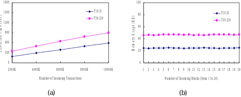
4.1 Scalability Study of DSM-FI
In this experiment, we examine the two primary factors, execution time and memory usage, for mining frequent itemsets in a stream environment, since both should be bounded online as time advances. Therefore, in Figure 9 (a), the execution time grows smoothly as the dataset size increases from 2,000K to 10,000K. The default value of minimum support threshold ms is 0.01%. The memory usage in Figure 9 (b) for both synthetic datasets is stable as time progresses, indicating the scalability and feasibility of algorithm DSM-FI. Notice that, the synthetic data stream used in Figure 9 (b) is broken into 20 blocks with size 50K. 0 300 600 900 1200 1500 1800 2000K 4000K 6000K 8000K 10000K
Number of Incoming Transactions
E xe cu ti on T im e (S ec .) T10.I5 T30.I20 (a) 0 20 40 60 80 100 1 2 3 4 5 6 7 8 9 10 11 12 13 14 15 16 17 18 19 20 Number of Incoming Blocks (from 1 to 20)
Me m or y U sa ge ( K B ) T10.I5 T30.I20 (b)
Figure 9. Required resources of DSM-FI for IBM synthetic datasets: (a) execution time, (b) memory usage 1 10 100 1000 10000 100000 2000K 4000K 6000K 8000K 10000K
Number of Incoming Transactions
E xec u ti on T im e ( sec .) DSM-FI Lossy Counting (a) 0 50 100 150 200 250 300 1 2 3 4 5 6 7 8 9 10 11 12 13 14 15 16 17 18 19 20 Number of Incoming Blocks (from 1 to 20)
Me m or y Us ag e (KB ) DSM-FI Lossy Counting (b)
4.2 Comparison with algorithm Lossy Counting
In this experiment, we examine the execution time and memory usage between DSM-FI and Lossy Counting by dataset T30.I20.D1M. In Figure 10 (a), we can see that the execution time incurred by DSM-FI is quite steady and is shorter than that of Lossy Counting. The experiment shows that DSM-FI performs more efficiently than Lossy Counting. In Figure 10 (b), the memory usage of DSM-FI is more stable and smaller than that of Lossy Counting. This is because DSM-FI does not need to enumerate all subsets of each incoming transaction. The amount of all subsets is an enormous exponential number for long transaction. Hence, it shows that DSM-FI is more suitable for mining long frequent itemsets in data streams.
5 Conclusions
In this paper, we proposed an efficient algorithm DSM-FI to find all frequent itemsets in data streams based on a landmark windows model. A new summary data structure IsFI-forest is developed for storing essential information about frequent itemsets of the streaming data seen so far. Experiments with synthetic data datasets show that DSM-FI is efficient on both sparse and dense datasets, and scalable to very long data streams. Furthermore, DSM-FI outperforms the well-known single-pass algorithm Lossy Counting for mining frequent itemsets over the entire history of the data streams.
References
1. R. Agrawal, T. Imielinski, and A. Swami. Mining Association Rules between Sets of
Items in Large Databases. In ACM SIGMOD Conf. Management of Data, 1993.
2. R. Agrawal and R. Srikant. Fast Algorithms for Mining Association Rules. In Conf. of the
20th VLDB conference, pages 487-499, 1994.
3. B. Babcock, S. Babu, M. Datar, R. Motwani, and J. Widom. Models and Issues in Data
Stream Systems. In Proc. of the 2002 ACM Symposium on Principles of Database Systems (PODS 2002), ACM Press, 2002.9.
4. J. Chang and W. Lee. Decaying Obsolete Information in Finding Recent Frequent
Itemsets over Data Stream. IEICE Transaction on Information and Systems, Vol. E87-D, No. 6, June, 2004.
5. J. Chang and W. Lee. A Sliding Window Method for Finding Recently Frequent Itemsets
over Online Data Streams. Journal of Information Science and Engineering, Vol. 20, No. 4, July, 2004.
6. C. Giannella, J. Han, J. Pei, X. Yan and P. S. Yu. Mining Frequent Patterns in Data
Streams at Multiple Time Granularities. In Proc. of the NSF Workshop on Next
Generation Data Mining, 2002
7. J. Han, J. Pei, and Y. Yin. Mining Frequent Patterns without Candidate Generation. In
Proc. of 2000 ACM SIGMOD, pages 1-12, 2000.
8. G. S. Manku and R. Motwani. Approximate Frequency Counts Over Data Streams. In
Proc. of the 28th VLDB conference, 2002.
9. W.G. Teng, M.-S. Chen, and P. S. Yu. A Regression-Based Temporal Pattern Mining
Scheme for Data Streams. In Proc. of the 29th VLDB Conference, 2003.
10. Y. Zhu and D. Shasha. StatStream: Statistical Monitoring of Thousands of Data Streams in Real Time. In Proc. 28th Int. Conf. on Very Large Data Bases, 2002.