生化資料的結構方程式模式分析; Analysis of Biochemical Data Using Structural Equation Model

全文

(1)Chapter 1 Introduction 1.1 Background From 1999 to 2000, a regular screening program was executed at Hsin-Yi rural area of Nantou County of Taiwan. This program targeted at several purposes. First, potential chronic disease patients could be traced and followed- up through this program since the resources and accompanied medical care are not well established in this area. Second, health-related interventions could be implemented via face-to-face interview and physical examinations. Third, an epidemiologic cohort of a health promotion plan and consecutive researches could be built on the basis of this cross-sectional sample. In this program, physical examinations, collection of serum and urine samples, as well as a questionnaire, were administrated on each person. The risk factors of several chronic diseases, including GOUT, hyperuricemia,..etc., have already been reported in Lai (2002).. Physiological phenomena and the motivation problem As we know that many chronic diseases are related with each other in that there might be one or even several common factors or latent variables involve in the mechanism of these diseases. Investigation of the relationship between factors is thus appealing in several aspects. (1) A further causal structure can be clarified if prospective data are available. (2) Prediction models (for early detection and treatment) of diseases can be set-up. (3) Confounding and/or variance component structure of an extra variable, the genetic factor for example, can be readily added. With this concern, we implemented a structural equation model (SEM) to explore the interrelations of physiological indices since they are closely related to each other group-by-group, along with a set of ‘baseline’ variables.. 1.

(2) Structural equation modeling Structural equation model ( SEM) is often used in psychometrics. It allows one to. evaluate causal hypotheses on a set of inter-correlated non-experimental data. Mathematically, SEM can be thought of as a combination of classical path analysis (possibly with latent variables) and the ‘confirmatory factor analysis (‘CFA’, or ‘measurement model’). Recently, the CFA have been proved suitable for evaluating the quality of blood pressure measurements other than the psychiatric data in early researches.( Batista-Foguet) It summarizes the relationships between latent. variables in a standard model or between risk factors and outcomes in ‘nonstandard model’. SEM techniques are distinguished by two characteristics: estimation of multiple and interrelated dependence relationships, and, more importantly, the ability to represent unobserved, conceptualized variables in these relationships and account for measurement errors in the estimation process.. 1.2. Goal of this study The collected data, which is described and explored in the ne xt chapter, contains various serum indices (including urine, GOT, GPT,… , etc.), physiological variables (including systolic pressure, diastolic pressure, WBC, RBC, … , etc.), the baseline variables, and some variables representing personal lifestyle in cigarette smoking, drinking, and betel nut eating. (In addition, genetic factors including family data are being collected.) If further information about the status of several chronic diseases such as GOUT, hypertention, DM, was available, these variables/risk factors can be used as predictors of disease under the follow- up study framework. To this end, a number of linear regression or prospective logistic regression models are usually used. That is, the physiological and biochemical measurement of an individua l may have power of prediction on several diseases. In the present study, however, no specific diseases status was diagnosed. So the main purpose of this article is to construct a primary model, an SEM, to build a possible inter-relation structure among these 2.

(3) variables.. This thesis is organized as follows. Chapter 2 reviews the role and characteristics of the serum biochemical measurements, and the notations and expressions of structural equation model (SEM). Motivations contrasting with the conventio nal analysis procedure are also addressed. Chapter 3 gives exploratory data analyses for the whole dataset. The results of univariate analyses and pair-wise correlations are reported. Note that the preliminary correlation matrix offers a naïve perspective of the multi-collinearity structure among the covariables, it paves way to a later factor analysis with latent variables. Chapter 4 gives the main result of this thesis, which suggests a two-stage algorithm of model construction. First, The ‘measurement model’ is constructed using a data-dependent exploratory factor analysis (EFA). Second, the structure of measurement model is employed in a construction of the entire structural equation model. In this procedure, goodness-of- fit (GOF) indices are the main criteria to give a valid, or at least, reliable modeling. The complexity of model building task always involves the inclusion and elimination of some variable(s) and/or factor(s). As a first step, we use a multivariate regression analysis for each primary ‘univariate’ variables or for each secondary factor score consisting of several primary variables in the same factor. Different rules for the assessment of contribution to the significance of a ‘factor’ can be used to select some possible models. As a final step, the marginal correlation structure of all observed variables serves as a tool to give a ‘final’ model, in terms of the GOF indices. In Chapter 5, we give some discussion about our results.. 3.

(4) Chapter 2 Notations and Literature Review 2.1 On the biochemical values In the natural history of a chronic disease, pre-clinical symptoms are usually not apparent to be diagnosed. In spite of this, a public-health concern is to seek for suitable indicators obtained from serum samples in regular examinations. Laboratory tests are then used as overall physical assessments to detect some abnormal results. Routinely performed tests include hemoglobin, red blood cell count, cholesterol, triglycerides, total lymphocyte count, serum albumin, etc. Other tests such as pla telet, globulin, glucose, AST, ALT, BuN, creatinine, and uric acid also provide non- ignorable information. In this thesis, all these values are called physiological or biochemical indices. They are used as variables to be classified into several groups or factors. In a general classification, white blood cell, red blood cell, hemoglobin, platelet are usually grouped together and treated as being related to the “function of blood manufacturing ”. A group of “cardiovascular function” includes systolic and diastolic blood pressures, cholesterol level, triglycerides, HDL-C/LDL-C. Another group related to “liver function” includes the synthesis of albumin and globulin, AST, and ALT. The other group of “kidney function” is composed of nitrogen balance, creatinine, serum uric acid and one about metabolism and nephritic absorption, blood sugar. In the following, we describe some characteristics and functions of these indicators.. Specific indicators (1) Uric acid is synthesized in liver, and excreted from kidney and intestine. In blood, a part of ion of uric acid combine with albumin, some exists with an ion type, and most of them exist in body fluid outside of vessel. The rates of decomposition and synthesis of protein balance each other. (2) Blood pressure (BP) is the force of the blood pushing against the side of 4.

(5) vessel wall. The systolic pressure is the maximum pressure felt on the artery during left ventricular contraction. The diastolic pressure is the elastic recoil, or resting, pressure that the blood exerts constantly between each contraction. These variations come from age, sex, race, rhythm, weight, exercise, emotions, stress, and so on. (3) Red blood cell count is the total number of hemoglobin per cubic millimeter in blood. The hemoglobin is an important part in red blood cell, and carries oxygen around our bodies. If a person suffers from anaemia, their red blood cell count and hemoglobin will always be under a normal level. (4) White blood cell count and type are the most commonly used tests of immune function. The number of white blood cells increases as a result of bacterial infection, bleeding, fever, inflammation, metabolism, and smoking and decreases due to antibodies which induce the autoimmune response. (5) Platelets are very small cells in the blood, and their major function is blood clotting. The decrease of platelets number will increase the chance of bleeding, even without injury. The mechanism involves autoimmune, chemotherapy, leukemia, viral infection, anaemia. An increase of number will make more blood clots, this involves bone marrow, splenectomy, etc. (6) Serum albumin and globulin make up most of proteins and their major functions are to provide nutrition for our body tissues. Hyperproteinemia is the major result of globulin. The albumin and globulin major synthesize in liver. In clinical aspects, decreases in concentration of albumin may due to hunger, malnutrition, synthesis velocity, liver cirrhosis, kidney syndrome, and infection, etc. (7) In human body, there are two important kinds of aminotransferase: aspartate oxaloacetate. transaminase. (GOT/AST),. and. alanine. pyruvate. transaminase. (GPT/ALT). They are used to detect the damage in liver. Note that GOT also exists in brain, heart, and blood cell, the increase in GOT- value may imply health problems of related organs. The major function of a liver relates to metabolism, storage, phagocytosis, and maintain plasma capacity and concentration. (8) Glycogen is the important part of sugar, and it stored by high concentration in 5.

(6) liver and muscle, and supplies the large number of energy for all body tissue by blood circulation. The glucose dissolution produces most of energy for the demand of human body. A greater part of the glucose in lipocyte will become lipide and be stored in lipidic tissues. Insulin can promote the glucose to form lipide. A part of the glucose in lipocyte changes to glycogen in the muscle tissues, and the process is also affected by insulin. As what is known, diabetes-status is a risk factor for the cardiovascular disease, and the cardiovascular disease can also lead to diabetes. A high level of blood sugar thus indicates problems in these organs or in hormone. (9) The lipids of human body contains triglyceride and cholesterol. Clinically, many diseases relate to lipoprotein change. Lipoprotein is a combination of lipid and protein (for example, triglyceride combines with alpha-globulin). Most of lipids combine with globulin. The sources of triglyceride and cholesterol are food and synthesized by liver. The causes of a high triglyceride level are due to diabetes, arteriosclerosis, kidney syndrome, hypothyroidism, hungry, diet, obesity, obstructive jaundice, acute/chronic pancreatitis, uremia, alcohol, hormone. The reasons for a low level are beta- lipoprotein deficiency, liver diseases, absorption deficiency syndrome, heparin use, or the problems in metabolism function. The value of serum triglyceride is age-dependent, and can be used for a screening of hyperlipidemia and to determine the risk of coronary artery disease. Moreover, total cholesterol is measured to evaluate fat metabolism and to assess the risk of cardiovascular disease. The normal range of a cholesterol level varies with age and gender. (10) Nitrogen balance (BuN) is a basic item of kidney examination, it is also an index of protein nutritional status. Nitrogen is released with the metabolism of amino acids, and the final production is urea. The concentration of BuN in blood is determined by protein ingestion and excretive rate of kidney. (11) Creatinine is derived from the breakdown of creatine through the synthesis of liver. It is not affected by protein ingestion and excreted unchanged in the urine at a constant rate. Thus the increase of concentration of creatinine in blood indicates the kidney function deficiency. The level of creatinine depends on individual weight, 6.

(7) height, gender, and age. It is sometimes viewed as an indicator of ageing. (12) Uric acid is released with metabolism of amino acid through purine. A high level of uric acid is due to hungry, obesity, hyperlipide ingestion, and alcohol. Hyperlipide produces ketone and alcohol restrains the excretive function of uric acid in kidney. Furthermore, diuretic, adrenalin, Niacin, Ethambutol, L-DOPA affect the uric acid le vel. The complication of hyperuricemia is an increase in red blood cell, leukemia, kidney function deficiency, or hypertension. The value of uric acid is also age-dependent.. The common ranges of the biochemical data Blood pressure : 120 ~ 159mmHg in SBP; 80 ~ 90mmHg in DBP. WBC (white blood cell) : 5000 ~9000/ul. RBC (red blood cell) : 4.5 ~ 5.5×106 /ul for male; 4.0 ~ 5.0×106 /ul for female. Hb (hemoglobin) : 14 ~ 18g/dl for male; 12 ~ 16g/dl for female. PLA (platelet) : 140 ~ 350×103 /ul. ALB (albumin) : 3.7 ~ 5.2 mg/dl. GLO (globulin) : about 2.4 mg/dl. Liver function: AST or ALT is higher than 40 U/ml and it is defined abnormal. BS (fasting blood sugar): 60 ~ 120 mg/dl. CHO (cholesterol level) : 130 ~ 225 mg/dl. Triglyceride is 25 ~ 150 mg/dl. The definition of hypertriglyceridemia is higher than 200mg/dl. In kidney function blood urea nitrogen is higher than 22mg/dl or creatinine is higher than 1.2mg/dl. Uric acid is 3.5 ~ 7.2mg/dl. It is abnormal when UA is higher than 7mg/dl for male or 6mg/dl for female.. 2.2 Notations Structural equation model (SEM) 7.

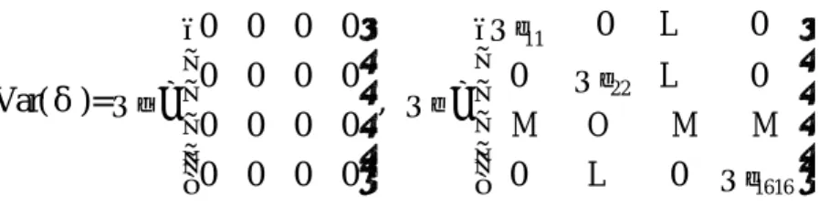
(8) Notations adopted in this thesis are the ‘LISREL notation’ system. The SEM is composed of two primary components: a structural model and a measurement model. The structural model is ? = G?+?. Two equations for the measurement model are y =? y ?+e and x =? x ?+d. There are two kinds of variables: endogenous variables and exogenous variables. ‘Endogenous ’ refers to variables that are influenced by other variables in SEM and ”exogenous ” describes variables that are determined outside of the model system. The ‘matrix’ expression of the SEM structure include three parts: the structural model, the measurement model, and the covariance matrices. In this section, we take Figure 2.1 as an illustration of our notations. Structural model:.  η1   γ 11     η2  =  0  η3   γ13  η   γ  4   14. γ 21 γ 31 0   ξ1  ς 1      0 0 γ 42   ξ2  ς 2  + 0 0 0   ξ3  ς 3      0 0 γ 44   ξ4  ς 4 . Measurement model:.  x1   1     x2  =  0  x3   0  x   0  4   y1   λ11     y2   M  y3   0     y4  =  M y   0  5   M  M y   0  16  . 0 1 0 0. 0 0 1 0. 0   ξ1  δ 1      0   ξ2  δ 2  + (ds can be equal to zero.) 0   ξ3  δ 3      1   ξ4  δ 4 . 0 0 M M λ52 0 M M λ83 0 M 0. M 0. 0   ε1     M ε2  η1    0    ε3    η M  2  + ε4  η  0   3   ε 5   η   M   4   M ε  λ164   16 . Covariance matrices:.  φ11  φ Var(X)= Φ =  21  φ31  φ  41. φ12. φ13. φ22 φ23 φ32 φ33 φ42 φ43. φ14  ψ 11  ψ φ 24  21 , Ψ = ψ 31 φ34    ψ φ 44   41 8. ψ12 ψ13 ψ 14  ψ 22 ψ 23 ψ 24  ψ 32 ψ 33 ψ 34   ψ 42 ψ 43 ψ 44 .

(9) 0 0 Var(δ)= Θδ =  0  0 . 0 0 0 0. 0 0 0 0. 0 L 0  0  Θε11    0 0 Θε 22 L 0   , Θε =  M O 0 M M       0 L 0 Θε1616   0. The y- variables are the 16 observed (measured) physio logical/biochemical indices which are expressed as y=?×?+e. The ?-variables are the latent endogenous variables with errors ?s. The x-variables are the exogenous variables obtained with or without errors. If there is no error (d) in x, then ?=x. The parameters of major interests to be estimated are ? (the factor loading of a ‘y’ with respect to an ’?’) and ? (the effect of an ‘x’ or ‘?’ on a factor ’?’). In order to obtain valid estimates, the covariance parameters are usually solved simultaneously with the parameters of interests. Finally, F and ? are covariances of ? and ?, respectively.. Fig. 2.1 An illustration of notations using an SEM structure obtained in Chapter 4.. 2.3 Literature review The SEM approach to statistical analysis is largely studied in econometrical and 9.

(10) psychometrical literatures as well as in behavioral sciences, clinical researches in nursing, and the field of hospital management, etc. General studies of development of SEM methodology include Bollen (1989), Mueller (1996), and Wan (2002). Bollen (2001) also provided a simple introduction to the theory, notations, and statistical issues of SEM. With SEM method, several systems of analysis packages (among others) have been developed: (1) SAS PROC CALIS (SAS Inc., Version 8.2) contains unconstrained estimation of measurement model (CFA) as well as the entire SEM. It provides generalized least squares (GLS option), weighted least squares (ADF option), and maximum likelihood estimates (ML option) in the MODEL statement. (2) LISREL (Jöreskog and Sörbom, 1992, LISREL 8) offers constrained estimation of CFA and SEM components. It is user friendly but suffers for convergence problem (in our experience!) if data analyzed is not suitably standardized in some situation. (3) EQS (Bentler, 1989) is developed as a simple version of LISREL.. In order to obtain a final structural model, first one has to obtain a measurement model based on a confirmatory factor analysis (CFA). The CFA framework is usually executed with the knowledge of which variable(s) should be grouped together and which should not. And then, based on the construct of the measurement model obtained from CFA, an SEM is fitted. There are two scenarios played in the procedures of constructing an SEM: the one -stage and two -stage approaches. In a one-stage approach (or simultaneous estimation), parameters are estimated through maximum likelihood method, for example, in a simultaneous estimation procedure, in which, however, a problem of non-convergence is often encountered. In a two-stage approach, on the other hand, the parameter in a measurement model (CFA) is firstly estimated and the entire part is then used as fixed to undergo the construct of a likelihood in the coming estimation. In our problem, however, there is no confirmatory part based on physiological 10.

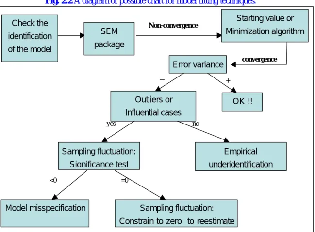
(11) reasons. It is thus appealing to use an exploratory factor analysis (EFA) and its corresponding result to build a measurement model. A question arises since the errors or residuals of an EFA are not correlated but those of a CFA are correlated. This induces a concern about the procedure of constructing a full SEM. In this thesis, we suggest a hybrid approach to the construction of the SEM by the following three steps: (I) To give an EFA analysis for the observed variables (y) in order to obtain a primary measurement model; (II) to construct the SEM according to some preliminary analyses on the inter-relations between the observed/latent variables; and (III) since the previous step introduces some correlations between the errors (or residuals), a correlation structure of the observed variables (y) is considered in a stepwise manner to improve the fit. We call this hybrid procedure a two-stage construct of SEM with a ‘simultaneous’ (rather than ‘two-stage’) estimation. For our dataset and whole research structure, population and family data of disease status, genotype, and other variables are still in collection. Before we can try to implement an SEM analysis on a future (more complete) dataset, an application of the SEM method to the present cross-sectional data serves as a premise to further statistical analysis. For example, on the stand of population-level, heritability estimation based on population and/or family data is of interest. (Pausova et al.2001). On a lower but more structured level, Province et al.(2001) use path analysis modeling to estimate familial aggregation and heritability; and Williams (1999) use a variance component analysis, along with the knowledge of genetic segregation, to give a linkage analysis. These also motivate our present study of SEM (using our present and future datasets).. For the techniques of implementing a system of structural equations, several aspects of data characteristics need to be checked. For example, if the observed variables are seriously skewed, a robust approach via transformation of variables can be considered (K.H.Yuan et al.2000). Second, if non-convergence problem and/or improper solution are encountered, guidelines of a model-building procedure have to be taken. 11.

(12) In what follows, we use the suggestion of Chen et al. (1999), which is summarized and expressed in the following diagram (Figure 2.2).. Fig. 2.2 A diagram of possible chart for model fitting techniques. Starting value or. Check the. Non-convergence. SEM. identification. Minimization algorithm. package. of the model. convergence. Error variance －. +. Outliers or. OK !!. Influential cases yes. no. Sampling fluctuation:. Empirical. Significance test. underidentification. <0. Model misspecification. =0. Sampling fluctuation: Constrain to zero to reestimate. 12.

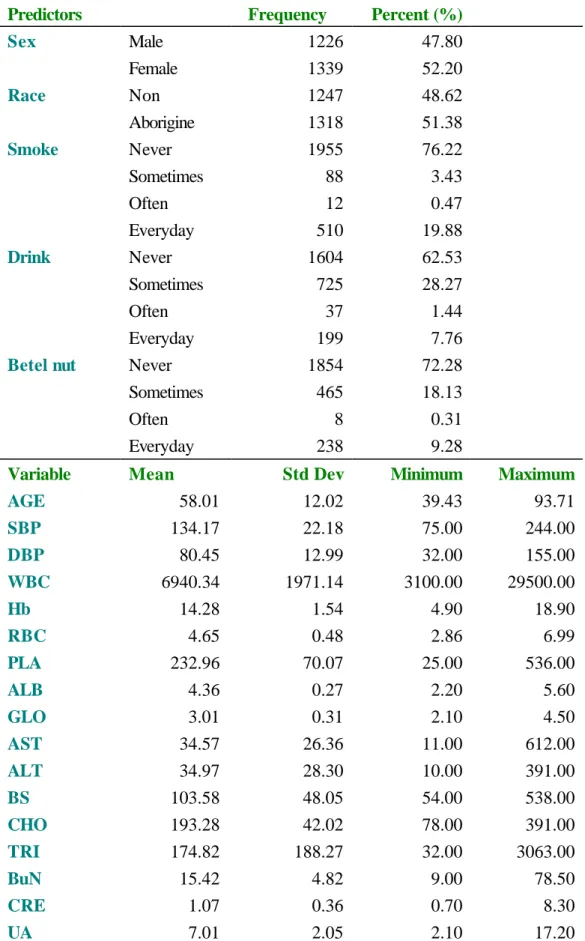
(13) Chapter 3 Materials and Preliminary Analyses 3.1 Dataset Our dataset is collected and offered by Dr. Li-Hsin Lai and his staff of health section of Hsin-Yi township, Nantou County of Taiwan. A cross-sectional community-based survey and screening program was conducted on 2,565 adult participants (aged 40 or older) during a health examination. Demographic data and variables concerning life-style are obtained from questionnaire; biochemical values are from blood extraction. The screening rate (or participation proportion) was 45.8%. There was no significant difference between the participants and non-participants in terms of the age, sex, and race structure/distributions of the whole township. In the sample, there were 1226 (47.8%) males and 1339 (52.2%) females, and 1318 (51.4%) aborigines and 1247 (48.6%) non-aborigines.. Covariables and measurements In our study, we used age, life-style (smoking, drinking, betel nut chewing) and as risk factors. In particular, they were treated as exogenous variables in the SEM context. Endogenous variables mainly consisted of the physiological and biochemical measurements such as systolic blood pressure (SBP), diastolic blood pressure (DBP), white blood cell (WBC), red blood cell (RBC), hemoglobin (Hb), platelet (PLA), albumin (ALB), globulin (GLO), AST (GOT), ALT (GPT), blood sugar (BS), cholesterol (CHO), triglyceride (TRI), blood urea nitrogenk (BuN), creatinine (CRE), and uric acid level (UA). These instruments included Sysmex-100 in blood examination, Hitach 704 in biochemical examination, UA by enzymatic-color method, blood sugar by oxidase method and cholesterol and triglyceride by oxidase--peoxidase method and glycorokinas- glycerophosphate-oxidase-peroxidase method, respectively. For all of the above measurements, they was performed by a standard checkout of lab condition.. 13.

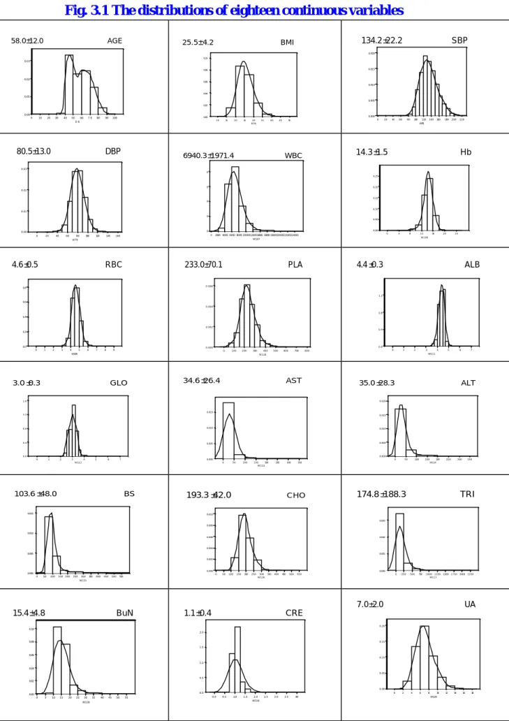
(14) 3.2 A preliminary of data analysis procedure As the first step of exploratory data analysis (EDA), the characteristics of all variables/covariables should be analyzed. There were three types of variables in our data: continuous variables (age and all physiological/biochemical measurements), indicator variables (sex and race), and ordinal variables (concerning life-style). Basically, all these variables are ‘primary’ or ‘directly observed’. In some researches, ‘secondary’ variable such as BMI is also considered as a confounder which is defined by other primary variables. In our analysis, we only study the linear relationship among all these directly observable variables so the secondary variables are not included in the analysis. For discrete variables, we presented frequencies; for continuous variables, sample means and standard deviations are calculated and histograms (with smoothing loess curve estimates) are plotted. Because the relationships among these physiological/biochemical value s are of interests, we presented the pairwise correlation matrix.. The second step is to construct the measurement model of an SEM. According to a previous context, there is no clear and evident classification for functional target of all the physiological/biochemical measurements of human body in clinical test, we used exploratory factor analysis (EFA) for the purpose of classification. The 16-item physiological/biochemical values were subjected to an exploratory factor analysis using the squared multiple correlations as prior communality estimates (L. Hatcher,. 1998). The maximum likelihood (ML) method was used to extract the factors, and ploted the factor pattern before rotation. The scree test and the rule of ‘eigenvalu-one’ suggested a solution of four factors that will be retained for further analysis ( L. Hatcher, 1998 ). As a result, factors 1 to 4 accounts for nearly 100% of the total sum of squares. This classification was then treated as being useful for further development of confirmatory factor analysis (CFA). The measurement model comprised of latent endogenous variable and observed endogenous variables; it was 14.

(15) tested and renewed until a statistically acceptable model, in terms of ‘good fits’, was obtained. In order to select a construct of SEM, we compared factor scores in EFA and CFA and carried out multiple linear regression analysis for each factor score. However, there were different choices of factor scores. For examples, Bartlett (1937,1938) and ˆ -1 Λˆ ( Λˆ ′ Ψ ˆ -1 Λˆ )-1 and Y=X Ψ ˆ -1 Λˆ (I+ Λˆ ′ Ψ ˆ -1 Λˆ )-1, Thomson (1951) suggested Y=X Ψ. respectively. The Bartlett’s score is hereafter referred to as a naïve method since ˆ -1/2 , Λˆ 0 = Ψ ˆ -1/2 Λˆ , Ψ ˆ is symmetric.) So the factor scores Y=V Λˆ 0 ( Λˆ ’0 Λˆ 0 )-1 . (V= X Ψ. produced by the naïve method could be compared to the Thomson’s scores. Next, we carried out multiple regressions for factor score each in individual. That means we only considered one response (dependent variable) at a time, and the response variable can be the unobserved latent factor or the observed physiological or biochemical measurements. From the analysis, we recorded significant level and used some criteria to produce a construct of measurement model. In the procedure of model fitting, several goodness-of-fit indices were employed as indices of model adequacy.. 3.3 Exploratory data analysis. Descriptive statistics Descriptive statistics, as well as the distributions, of all exogenous and endogenous variables are reported in Table 3.1 and Figure 3.1. The joint distribution of sex and race of this sample is not significantly different from the distribution of the entire Hsin-Yi area for those aged 40 or older. Concerning the life-style variables, there are 76.22% of nonsmoking, 62.53% of non-drinking, and 72.28% of people without chewing betel nut. The mean age is 58.01 years old (standard deviation= 12.02); the mean and standard deviation for physiological/biochemical values are 134.17±22.18 mmHg (SBP), 80.45±12.99 mmHg (DBP), 6940.34±1971.14 /ul (WBC), 14.28±1.54 g/dl (Hb), 4.65±0.48 ×106 µl (RBC), 232.96±70.07 (PLA), 4.36±0.27 mg/dl (ALB), 3.01±0.31 mg/dl (GLO), 34.57±26.36U/ml (AST), 15.

(16) 34.97±28.30 U/ml (ALT), 103.58±48.05 mg/dl (BS), 193.28±42.02 mg/dl (CHO), 174.82±188.27 mg/dl (TRI), 15.42±4.82 mg/dl (BuN), 1.07±0.36 mg/dl (CRE), 7.01±2.05 mg/dl (UA), respectively. To compare with the common range, we found that most of the observations falls into the common range except for uric acid. The uric acid level is obviously higher than the general population. Health-related problems of this community such as hyperuricemia and gout are thus important.. Pairwise correlation matrix Conventional factor analysis and principal component analysis rely heavily on the structure of inter-correlations among the variables studied. By calculating the pairwise correlations of physiological/biochemical data, it offers insight into the factor analysis. For example, SBP and DBP are both used to check the blood pressure and they surely have a high correlation. Similarly, AST and ALT, Hb and RBC, BuN and CRE, are used to check the liver function, blood function/anemia, and kidney function respectively. All pairs have high correlations. We draw the color with dark or light to represent different levels of correlations. By a suitable alignment, the pattern of clusters could be determined from the correlation matrix. Nonetheless, some mathematical techniques is yet developed (at least in this thesis) and compared to the conventional principal component analysis (PCA) or factor analysis. From this matrix, on the other hand, we only distinguished (roughly) four clusters from PCA (Table 3.2). The variables SBP, DBP, WBC, and CHO are treated as from a factor connected with cardiovascular function; the variables GLO, AST, and ALT are grouped and thought to be associated with liver function. We continued this process to group Hb, RBC, PLA, ALB, and TRI, connected with manufacture blood function, or quality of blood. Finally, BS, BuN, CRE, and UA are combined into one group correlated with metabolism, excrete, and kidney function. These groupings will be further checked and confirmed by exploratory factor analysis reported in the next chapter.. 16.

(17) Table 3.1 Descriptive statistics of the exogenous and endogenous variables Predictors Sex Race Smoke. Drink. Betel nut. Variable AGE SBP DBP WBC Hb RBC PLA ALB GLO AST ALT BS CHO TRI BuN CRE UA. Male Female Non Aborigine Never Sometimes Often Everyday Never Sometimes Often Everyday Never Sometimes Often Everyday Mean 58.01 134.17 80.45 6940.34 14.28 4.65 232.96 4.36 3.01 34.57 34.97 103.58 193.28 174.82 15.42 1.07 7.01. Frequency 1226 1339 1247 1318 1955 88 12 510 1604 725 37 199 1854 465 8 238. Percent (%) 47.80 52.20 48.62 51.38 76.22 3.43 0.47 19.88 62.53 28.27 1.44 7.76 72.28 18.13 0.31 9.28. Std Dev 12.02 22.18 12.99 1971.14 1.54 0.48 70.07 0.27 0.31 26.36 28.30 48.05 42.02 188.27 4.82 0.36 2.05. Minimum 39.43 75.00 32.00 3100.00 4.90 2.86 25.00 2.20 2.10 11.00 10.00 54.00 78.00 32.00 9.00 0.70 2.10. 17. Maximum 93.71 244.00 155.00 29500.00 18.90 6.99 536.00 5.60 4.50 612.00 391.00 538.00 391.00 3063.00 78.50 8.30 17.20.

(18) Fig. 3.1 The distributions of eighteen continuous variables 58.0±12.0. AGE. 25.5±4.2. 134.2± 22.2. BMI. SBP. 0.020 0.10. 0.03 0.015. 0.08. 0.02 0.06. 0.010. 0.04. 0.01 0.005 0.02. 0.00 0. 10. 20. 30. 40. 50. 60. 70. 80. 90. 0.000. 0.00. 100. 10. E6. 80.5± 13.0. DBP. 15. 20. 25. 30 B76. 35. 40. 45. 0. 50. 20. 40. 60. 80. 100. 120. 140. 160. 180. 200. 220. W78. 6940.3±1971.4. 14.3± 1.5. WBC. Hb. 0.03. 0 0.25. 0. 0.20. 0.02 0.15. 0 0.10. 0.01. 0 0.05. 0.00. 0. 0.00 0. 20. 40. 60. 80. 100. 120. 140. 0. 160. 0. 2000 4000 6000 8000 100001200014000 16000 18000200002200024000. 4. 8. 12. 4.6± 0.5. 233.0±70.1. RBC. 16. 20. 24. W108. W107. W79. PLA. 4.4± 0.3. ALB. 0.006. 0.8. 1.2 0.6. 0.004 0.8 0.4. 0.002 0.4 0.2. 0.0. 0.0. 0.000 0. 1. 2. 3. 4. 5. 6. 7. 8. 9. 0. 100. 200. 300. 400. W109. 500. 600. 700. 0. 800. 1. 2. 3. 3.0± 0.3. GLO. 4. 5. 6. 7. W111. W110. 34.6± 26.4. AST. 35.0± 28.3. ALT. 0.020. 1.6. 0.015 1.2. 0.015. 0.8. 0.010. 0.010. 0.4. 0.005. 0.005. 0.000. 0.0 0. 1. 2. 3. 4. 5. 6. 0.000. 7. 0. 0. W112. 103.6±48.0. BS. 50. 100. 150 200 W113. 250. 300. 193.3± 42.0. 0.015. 50. 100. 150. 350. CHO. 200 W114. 250. 300. 174.8± 188.3. 350. TRI. 0.010. 0.003 0.008. 0.010 0.002. 0.006. 0.004. 0.005. 0.001 0.002. 0.000. 0.000. 0.000. 0. 0. 50. 100. 150. 200. 250. 300. 350. 400. 450. 500. 50. 100. 150. 200. 250. 550. 300 W116. 350. 400. 450. 500. 0. 550. 250. 500. 750. 1000 1250 W117. 1500. 1750. 2000. 2250. W115. 7.0±2.0. 15.4±4.8. BuN. 1.1±0.4. UA. CRE 0.20. 0.10 2.0. 0.08. 0.15. 1.5. 0.06 0.10. 1.0. 0.04 0.05. 0.5. 0.02 0.00. 0.0. 0.00 0. 5. 10. 15. 20. 25. 30. 35. 40. 45. 50. 55. 0. 0.0. 0.5. 1.0. 1.5. 2.0 W119. W118. 18. 2.5. 3.0. 3.5. 4.0. 2. 4. 6. 8. 10 W120. 12. 14. 16. 18.

(19) Table3.2 Pairwise correlation matrix for 16 physiological/biochemical variables variables SBP. SBP. DBP. WBC. CHO. GLO. AST. ALT. Hb. RBC. PLA. ALB. TRI. BS. BuN. CRE. DBP. 0.7695 <.0001 0.1095 <.0001 0.1009 <.0001 0.0907 <.0001 0.0205 0.2996 0.0336 0.0889 0.0575 0.0036 0.0304 0.1234 -.0294 0.1360 0.0353 0.0743 0.0849 <.0001 0.0762 0.0001 0.0557 0.0048 0.0726 0.0002 0.1008 <.0001. 0.1195 <.0001 0.0934 <.0001 0.0780 <.0001 0.0143 0.4680 0.0356 0.0712 0.1228 <.0001 0.0940 <.0001 0.0154 0.4360 0.0667 0.0007 0.1263 <.0001 0.0576 0.0035 0.0049 0.8058 0.0668 0.0007 0.1410 <.0001. 0.0970 <.0001 0.1046 <.0001 -.0161 0.4153 0.0573 0.0037 0.1116 <.0001 0.0871 <.0001 0.2075 <.0001 0.0603 0.0022 0.0744 0.0002 0.0415 0.0357 0.1629 <.0001 0.0870 <.0001 0.2197 <.0001. 0.0337 0.0882 -.0631 0.0014 -.0051 0.7947 0.1243 <.0001 0.0903 <.0001 0.1125 <.0001 0.1953 <.0001 0.3105 <.0001 0.0759 0.0001 0.1383 <.0001 0.0506 0.0103 0.0401 0.0424. 0.2267 <.0001 0.1830 <.0001 -.0316 0.1098 -.0914 <.0001 0.0136 0.4918 -.0338 0.0872 0.1643 <.0001 0.1094 <.0001 0.0227 0.2496 0.0031 0.8768 0.1981 <.0001. 0.7549 <.0001 0.0729 0.0002 -.0660 0.0008 -.0982 <.0001 -.0921 <.0001 0.1267 <.0001 0.0462 0.0193 -.0712 0.0003 -.0175 0.3761 0.1752 <.0001. 0.1487 <.0001 0.0403 0.0411 -.0787 <.0001 0.0225 0.2552 0.1233 <.0001 0.0933 <.0001 -.0497 0.0118 -.0189 0.3396 0.1605 <.0001. 0.6044 <.0001 -.1423 <.0001 0.2713 <.0001 0.1287 <.0001 0.0509 0.0099 -.1474 <.0001 -.0235 0.2347 0.2028 <.0001. -.0286 0.1477 0.3096 <.0001 0.0072 0.7163 0.0140 0.4774 -.1286 <.0001 -.0485 0.0140 0.0699 0.0004. 0.0994 <.0001 0.0751 0.0001 -.0363 0.0658 -.0256 0.1949 -.0330 0.0950 0.0653 0.0009. 0.0805 <.0001 0.0115 0.5622 -.0125 0.5267 -.0227 0.2503 -.0010 0.9592. 0.2709 <.0001 -.0034 0.8653 0.0305 0.1220 0.2496 <.0001. 0.0696 0.0004 0.0541 0.0062 -.0132 .5043. 0.5837 <.0001 0.1751 <.0001. 0.2061 <.0001. WBC CHO GLO AST ALT Hb RBC 19. PLA ALB TRI BS BuN CRE UA. UA.

(20) Chapter 4 Statistical Analysis and Main Results In sociological researches, often there is a hypothetical structure, which is referred to as a ‘model’, and data or information collection is processed through a (structured) questionnaire and accompanied statistical analysis to validate the model. The most common adopted statistical method is the structural equation modeling (SEM). However, it should not be a paradigm since this ‘model’ or ‘procedure’ a priori of scientific research tells no more story than a result obtained from that without a model assumption. That means, a scientific model could also be set-up by a procedure with a ‘meta’-sense in that we can still build a posterior model after the analysis is completed, if there is some interpretability concerning the results.. For our health-related data, it is still lack of theoretical support and physiological/pathological evidence or reasons that which variables should be grouped together and, likewise, the mechanism and causal results of a variables/index on the other(s) and their recursive relationships are also unknown. For a set of variables collected from a cross-sectional sample consisted of aged people, the inter-relations between variables may have different pattern from the reasoning of physiological/pathological aspects. For example, SBP, DBP, and WBC grouped in a factor cannot be over- interpreted in that they do have causal relationship in the formation of chronic diseases. On the other hand, they should be viewed as being common results related to an unknown, unobservable pathway through a latent factor. In this regard, a confirmatory factor based on medical knowledge and an exploratory factor reflected from a ‘prevalence data’give no confliction.. 4.1 The measurement model in SEM There is a question about the ‘adequacy’ of giving a factor analysis before it is executed. To this end, a Kaiser’s pre-analysis measure can serve to judge the ‘level’ 20.

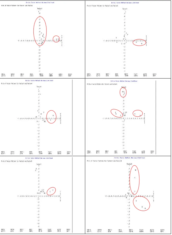
(21) of adequacy. For our data, the overall MSA (measure of sampling adequacy) is 0.563 and variable-specific measures are: SBP DBP WBC CHO. GLO AST ALT Hb. 0.52. 0.58. 0.77. RBC PLA ALB. TRI. BS. 0.60. 0.59. 0.52. 0.53. 0.44. 0.63. 0.71. 0.53. 0.54. 0.58. BuN CRE UA 0.52. 0.55. 0.65. As an usually experience, the level of 0.5 is recognized as an lowest acceptable threshold; and the level of 0.7 or above as being promising for a good factor analysis (H-J Chiou). It is noted from the above result that most of the ‘adequacy’ level lie within 0.5 to 0.6, the level of PLA is 0.44, and those of GLO and ALB are greater than 0.7. It is treated as being feasible to undergo a factor analysis. Another measure of sampling adequacy is the communality, which will be discussed later for specific models. In an exploratory factor analysis, each observed variable y1 , y2 , … , yp of a centered random vector y is assumed to be a linear combination of m factors f1 , f2 , … , fm : y1 -μ 1 =λ 11 f1 +λ 12 f2 + … +λ 1m fm +ε 1 y2 -μ 2 =λ 21 f1 +λ 22 f2 + … +λ 2m fm +ε 2 … … … … yp-μ p=λ p1 f1 +λ p2 f2 + … +λ pm fm +ε p. The coefficientsλij is referred to as the loading of factor j (fj) on the i-th observed variable yi. Ifλi1 is close to zero, for example, it means that the level of yi which is attributable to factor 1 (f1 ) is nearly zero or at least very non-significant. Moreover, with the above expressions, each yi represents a ‘point’ in the space spanned by factors (f1 ,f2 ,… ,fm). A suitable presentation of the ‘position’ of the point with respect to an (fi,fj)-pair can reveal comparative factor loadings between fi and fj of the variable concerned. If one plots the point of a variable yk in the fi-fj plane, for example, and if the position of yk is very close to the fi-axis, then the factor loading of yk with respect to fi is much larger than that of fj. In this case we believe that the ‘path’ from fi. 21.

(22) to yk should be considered, and the path from fj to yk may not be an important one. However, if the location of yk is just between the two axes (or lies around the line fi=fj), it means that both of the pathways from the two factors to the variable yk should be considered. The exploratory factor analysis (EFA) suggested four factors according to at least one of the following four criteria: eigenvalue -one criterion, the scree-plot diagnostics, the attributable proportion of (centered) sum of squares, and the ‘interpretability’ criterion. Of course, more factors also could be considered if the ‘interpretability’ criterion is greatly emphasized. In an analysis not reported in the context, most of measurement models based on more factors with a great physiological assortment and interpretability do not converge even under a low decimal criterion. The resultant classification of the 16 physiological/biochemical values into four factors is as follows. Table 4.1 A classification according to exploratory factor analysis. Variables (y) Factor 1 (f1 ). GLO, AST, ALT. Factor 2 (f2 ). SBP, DBP, WBC, CHO. Factor 3 (f3 ). Hb, RBC, PLA, ALB, TRI. Factor 4 (f4 ). BS, BuN, CRE, UA. The plots of each ‘y’-variables on various fi- fj planes are shown in Figure 4.1. By careful examinations, one can check the above classification through the six plots in that which variable (y) is reasonably classified into which factor (f), as well as the co-influence of two or more factors on the same variable (y). For example, the points A and B (SBP and DBP) are almost no doubt to be classified as Factor 2 (f1 ), but the point C (WBC) can be attributed by Factor 2 (f1 ) and Factor 4 (f4 ). The latter suggested a possible path from Factor 4 to WBC in the measurement model or SEM analysis. Similarly, the points D and E (Hb and RBC) both can be co-attributed by Factors 3 and 4, and so paths from Factor 4 to Hb and RBC are then possible.. 22.

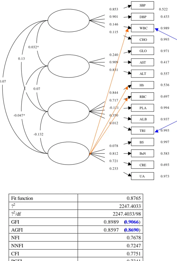
(23) Unfortunately, however, later analyses of measurement model and SEM with these ‘inter- factor relationship’ usually resulted in improper solutions, non-convergence estimates, and/or worse fits. At a request of parsimony when improper solutions are encountered (Chen, Bollen, et al., 1999), hereafter we will not take the case of ‘inter- factor relationship’ into consideration in our presentation and analysis. Figure 4.2 gives the estimates associated with the EFA of Table 4.1. When the biggest marginal correlation (CHO and TRI) among the observed variables is considered, goodness-of- fit indices (GFI and AGFI) were improved to a satisfactory level; though, substantial changes in the estimates of each factor loadings are not observed. This construct will be used as an initial ‘guess model’ for later modeling of SEM except for that more of the inter-variable correlations could be included to improve the fits. Finally, it is worth noting that the pairwise correlation matrix of Table 3.2 gives a contrast with the results of exploratory factor analysis of Table 4.1. [Put Figures 4.1 and 4.2 about here.]. 4.2 The structural model in SEM As a primary hypothesis, we assumed that the physiological/biochemical mechanism is not different between races and genders. With this assumption, we did not take race and gender as exogenous variables to make things simple and then the whole dataset was used to pursuit a reasonable model-building procedure in SEM. When it is believed that there is different among genders and/or races, however, more complicated fitting can be considered. For example, a ‘stratification’ on gender or race is possible.. Full model Since the inter-relationship between the four factors, reduced from 16 observed variables, and four risk factors or risk taking behaviors is of major concern, first we draw all possible paths as an initial construct of SEM. It is hereafter referred to as the full model. The fit of full model is not a good one (GFI=0.6808, NFI=0.0452, 23.

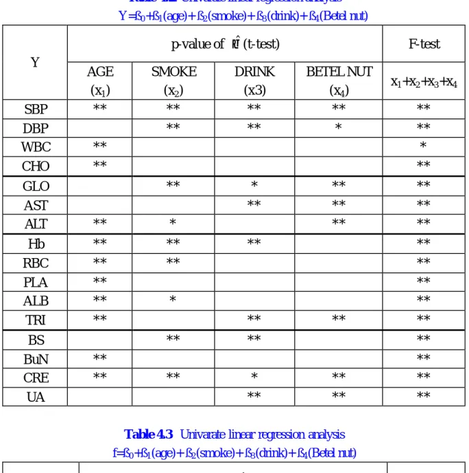
(24) CFI=0.0424). Standardized parameter estimates are presented in Figure 4.3. In order to improve the fit (in terms of goodness-of-fit indices), significant paths from the exogenous variables to the latent factors (terms as the γ-path) need to be identified and non-significant paths to be deleted. Traditional method concerning this ‘model-selection’ procedure is to use the Lagrange multiplier test (a parallel of Rao’s score test in regression set-up when there exists a likelihood) or the Wald test in a stepwise manner. However, when the likelihood of an SEM is written, it involves the whole structure of the SEM, including all the covariance parameters, γ-paths, and λ-paths (from factors to the observed y variables). This implies that the stepwise procedure involves a simultaneous estimation of all parameters, not only theγ-paths (orγ-parameters). In this thesis, we propose that the construct of an SEM as a two-stage procedure, but the estimation is a simultaneous one. In this regard, an alternative (but naïve) algorithm based on the two-stage thinking is proposed based on the building stone of univariate-multiple linear regression. ‘Univariate’ means that the outcome can be (i) the univariate observed variable, y, or (ii) a combined factor score; ‘multiple’ indicates that the explanatory variables are the set of risk factors (AGE, SMK, DRI, and PEA). For (ii), we use the naïve score proposed by Bartlett (1937) in which factor loadings are substituted by those parameter estimates obtained from the ML estimation of measurement model. There is another factor score suggested by the SAS system and, for the current dataset, scatter-plots (Figure 4.4) of these two factor scores shows that these two scores are high surrogates to each other. [Put Figures 4.3 and 4.4 about here.]. Univariate linear regression with observed dependent variables We used the physiological/biochemical variables as outcome variables and risk factors as predictors and proceeded regression analyses. In this process, we considered one responser (dependent variable) at a time, and the model could have many predictors (independent variables), so it is called a univariate multiple regression analysis. According to the analysis, we recorded the significant level and 24.

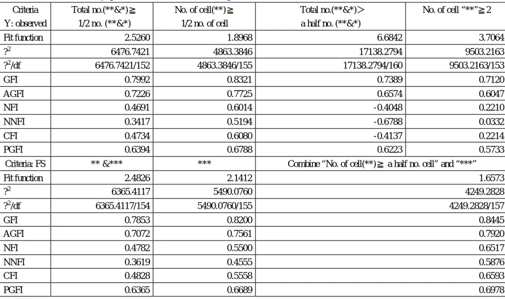
(25) provided some criteria to decide the structural model. The double asterisks represented the p-value less than 0.01, and one asterisk indicated a p-value within 0.01 to 0.05. In each cell, a ‘double asterisks’ is treated as being a full mark. The result of univariate multiple regression analysis was reported in Table 4.2. Next, total numbers of asterisks of x’s (age, smoking, drinking, and betel nut eating) on every observed variable (y) were counted for each factors (f). After this, various criterion rules can be used. (Note that each criterion rule corresponds to a construct.) Examples of considerations on the rules and their interpretation are as follows. (1) Additive-1/2 rule : The total number of asterisks is greater than or equal to a half of the possible number of asterisks. In this case, the corresponding γ-path is identified as being important. For example, from Table 4.2, since Factor 1 (f1 ) consisted of 4 variables, thus there must be 8 possible asterisks in 4 cells for each of the 4 risk factors. As a result, the age-f1 relation has 6 asterisks, reveals that the γ-path from AGE to Factor 1 should be considered. Similarly, theγ-paths from SMOKE and DRINK to Factor 1 are both important, but that from BETEL NUT to Factor 1 is not. This criterion relies on the additive effect of significance attributed from the relationship between risk factors (x) and distinct observed variables (y). (2) Relative significance rule: If the number of cells (which equals the number of variables related to a factor) with two-asterisks significance level exceeds, or equals to, the total number of cells, the γ-path is considered. This rule is very strict in asking for parsimony in the construct ofγ-path. (3) Strict additive-1/2 rule : Like the rule of (1) except for that the ‘equal to’-requirement is cancelled. (4) Absolute significance rule : When the number of cells with two-asterisks significance level exceeds 2, it is also reasonable to treat the factor to be highly attributable to the x variables in the sense that there are genuine contributions from x to the combined observed variables (y) which consisted of the factor (f). It is important to note that some variants of (1)~(4) or their configurations are also possible. (For details, please refers to the results of Table 4.4.) 25.

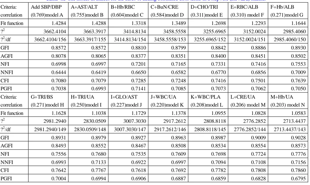
(26) Univariate linear regression with latent factor scores When the naïve factor scores were used as outcome variables, the case of p-value less than 0.01 were further partitioned into two sub-cases: 0.001<p< 0.01 and p< 0.001. We set 3 asterisks to the case of p- value<0.001, 2 asterisks to the case of 0.001<p< 0.01, and 1 asterisk to tha t of 0.01<p< 0.05. The result was presented in Table 4.3. [Put Tables 4.2 and 4.3 about here.]. According to the results of multiple regression analyses, we borrowed the criterion of relative significance rule. (i) If the number of cells (which equals the number of variables related to a factor) with 2 or more asterisks, or, (ii) if, in a more restrict sense, the number of cells with 3 asterisks exceeds or equals to the total number of cells, the γ -path is considered. The first consideration gives the following goodness-of- fit indices: GFI=0.7853, NFI=0.4782, CFI=0.4828; The second one gives GFI=0.8200, NFI=0.5500, CFI=0.5558.. As a final construct by combining the above results, we obtained an SEM shown in Figure 4.5 with the best goodness-of-fit indices with GFI=0.8445 and AGFI=0.7920. [Put Table 4.4 and Figure 4.5 about here.]. Adding/deleting correlated error terms stepwisely In order to obtain a satisfactory fit, in terms of goodness-of-fit indices, we tried to add the path of correlations between error terms of observed variables (y) in the order from high to low level of marginal correlations (though partial correlation also could be considered). We had the following order of correlations: SBP/DBP (0.769), AST/ALT (0.755), Hb/RBC (0.604), BuN/CRE (0.584), CHO/TRI (0.311), RBC/ALB (0.310), Hb/ALB (0.271), TRI/BS (0.271), TRI/UA (0.250), GLO/AST (0.227), 26.

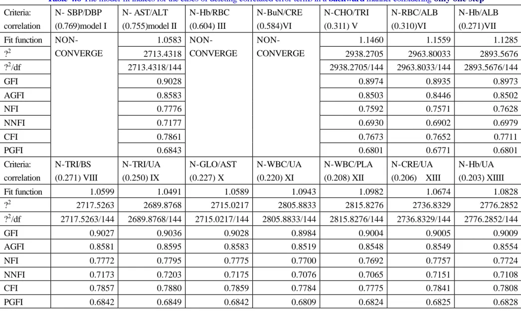
(27) WBC/UA (0.220), WBC/PLA (0.208), CRE/UA (0.206), Hb/UA (0.203). According to this order, we added the path between variables (y) one at a time. This is why we called it a ‘stepwise’ manner. It is very different from the standard procedure suggested by most of the statistical packages that the selection of path is decided by a Wald test or a Lagrange multiplier test. The reason is, as stated previous ly, we seek to add the path(s) by a ‘two-stage’ manner. After the global structure is constructed, we can add the correlation terms by considering the ‘correlations’ between the observed variables (y) to raise the goodness-of- fit indices (GFI or AGFI, etc.) to a acceptable level. As suggested by this thesis, the primary pairwise (marginal) correlations can be used in a descending order. The result is shown in Table 4.5, in which adding the marginal correlation greater than 0.2 will finally give a GFI index greater than 0.90. On the other hand, if the Lagrange multiplier test is used from this stage (as suggested by the statistical packages) without regards to the parts other than the correlations between error terms, a model-building procedure can also be adopted. We contrasted these two procedures, in terms of the GFI/AGFI index, by Figures 4.6 and 4.7, respectively. It demonstrates the growth rate of GFI/AGFI and tells the betterment of our procedure at the early inclusion of higher correlations. Nonetheless, the Lagrange multiplier test still gives better fits from some step although it still falls into the framework of ‘two-stage’ modeling. Before a ‘final’ model is obtained, we can still investigate the ‘lack-of-fit’problem in what the change is when deleting a correlation between the observed variables (y). The results are reported in Table 4.6 and Figure 4.8. Finally, the magnitude of GFI-change when deleting one path of correlation in a ‘backward’ manner is shown in Figure 4.8; and a ‘final’ model is given in Figure 4.9. [Put Tables 4.5 and 4.6 about here.] [Put Figures 4.6, 4.7, 4.8, and 4.9 about here.]. 27.

(28) 4.3 Enhancing the model As stated in a previous context, there may be sex and/or race difference in the distributions of indicator variables of serum sample, but the mechanism or structure among all variables discussed is believed to be the same. There are at least two ways to deal with the effect of causal or confounding effect introduced by sex and race. They are very similar to the discussion in regression setting of statistical and epidemiological fields in which we consider two ways of treating confounding effect. Hereafter, we will further consider variables age and race to enhance the power and feasibility of an SEM model. That is, to add the sex/race variable into the structure as an exogenous variable or to use sex/race as a stratification variable. We illustrate the case of using race as an exogenous variable and sex as a stratification variable. Model building procedure follows what has been taken in this chapter except for the third step of adding correlations between observed variables (y) is neglected. The results are shown in Figures 4.10 and 4.11. Comparison of parameter estimates of different genders are attached at the end of these two figures using SAS PROC CALIS (unconstrained estimates). [Put Figures 4.10 and 4.11 about here.]. 28.

(29) Table 4.2. Univarate linear regression analysis Y=ß0 +ß1 (age)+ ß2 (smoke)+ ß3 (drink)+ ß4 (Betel nut). p-value of βˆ (t-test) Y. SBP DBP WBC CHO. AGE (x1) **. SMOKE (x2) ** **. DRINK (x3) ** **. BETEL NUT (x4) ** *. **. * **. ** ** **. ** ** **. **. ** ** ** ** **. ** **. ** ** ** **. ** **. GLO AST ALT. **. *. Hb RBC PLA ALB TRI. ** ** ** ** **. ** **. BS BuN CRE UA. F-test. **. * **. ** **. **. **. **. * **. x1+x2+x3+x4 ** ** * **. Table 4.3 Univarate linear regression analysis f=ß0 +ß1 (age)+ ß2 (smoke)+ ß3 (drink)+ ß4 (Betel nut). p-value of βˆ (t-teast) Y. FACTOR1 FACTOR2 FACTOR3 FACTOR4. AGE (x1) *** *** ***. SMOKE (x2) *** ** ***. DRINK (x3) *** ***. F-test BETEL NUT (x4) * *** ***. ***：p<0.001 ** ：0.001<p<0.01 * ：0.01<p<0.05. 29. x1+x2+x3+x4 *** *** *** ***.

(30) Table 4.4 To determine theγ-paths based on univariate linear regressions and several rules Criteria Y: observed. Total no.(**&*)≧ 1/2 no. (**&*). Fit function. No. of cell(**)≧ 1/2 no. of cell. Total no.(**&*)＞ a half no. (**&*). No. of cell “**”≧2. 2.5260. 1.8968. 6.6842. 3.7064. 6476.7421 6476.7421/152. 4863.3846 4863.3846/155. 17138.2794 17138.2794/160. 9503.2163 9503.2163/153. GFI. 0.7992. 0.8321. 0.7389. 0.7120. AGFI NFI. 0.7226 0.4691. 0.7725 0.6014. 0.6574 -0.4048. 0.6047 0.2210. NNFI. 0.3417. 0.5194. -0.6788. 0.0332. CFI PGFI. 0.4734 0.6394. 0.6080 0.6788. -0.4137 0.6223. 0.2214 0.5733. 2. ? ?2 /df. 30. Criteria: FS Fit function ?2. ** &***. ***. Combine “No. of cell(**)≧ a half no. cell” and “***”. 2.4826 6365.4117. 2.1412 5490.0760. 1.6573 4249.2828. 6365.4117/154. 5490.0760/155. 4249.2828/157. GFI AGFI. 0.7853 0.7072. 0.8200 0.7561. 0.8445 0.7920. NFI. 0.4782. 0.5500. 0.6517. NNFI CFI. 0.3619 0.4828. 0.4555 0.5558. 0.5876 0.6593. PGFI. 0.6365. 0.6689. 0.6978. ?2 /df.

(31) Table 4.5 The model-fit indices for the cases of adding correlated error terms in a stepwise (forward) manner Criteria: correlation Fit function. Add SBP/DBP (0.769)model A. A+AST/ALT (0.755)model B. B+Hb/RBC (0.604)model C. C+BuN/CRE (0.584)model D. D+CHO/TRI (0.311)model E. E+RBC/ALB (0.310) model F. F+Hb/ALB (0.271)model G. 1.4284. 1.4288. 1.3318. 1.3489. 1.2698. 1.2293. 1.1644. 3662.4104 3662.4104/156. 3663.3917 3663.3917/155. 3414.8134 3414.8134/154. 3458.5558 3458.5558/153. 3255.6965 3255.6965/152. 3152.0024 3152.0024/151. 2985.4060 2985.4060/150. GFI. 0.8572. 0.8572. 0.8810. 0.8799. 0.8842. 0.8886. 0.8930. AGFI NFI. 0.8078 0.6998. 0.8065 0.6997. 0.8377 0.7201. 0.8351 0.7165. 0.8400 0.7331. 0.8451 0.7416. 0.8502 0.7553. NNFI. 0.6444. 0.6419. 0.6650. 0.6582. 0.6770. 0.6856. 0.7009. CFI PGFI. 0.7080 0.7038. 0.7079 0.6993. 0.7285 0.7141. 0.7248 0.7085. 0.7416 0.7073. 0.7501 0.7062. 0.7639 0.7050. 2. ? ?2 /df. 31. Criteria: correlation Fit function ?2. G+TRI/BS (0.271)model H. H+TRI/UA (0.250)model I. I+GLO/AST (0.227)model J. J+WBC/UA (0.220)model K. K+WBC/PLA (0.208)model L. L+CRE/UA M+Hb/UA (0.206) model M (0.203) model N. 1.1628 2981.2940. 1.1038 2830.0509. 1.1729 3007.3030. 1.1378 2917.2612. 1.0955 2808.8118. 1.0828 2776.2852. 1.0583 2713.4437. 2981.2940/149. 2830.0509/148. 3007.3030/147. 2917.2612/146. 2808.8118/145. 2776.2852/144. 2713.4437/143. GFI AGFI. 0.8931 0.8493. 0.8979 0.8552. 0.8927 0.8467. 0.8963 0.8508. 0.8987 0.8534. 0.9009 0.8554. 0.9028 0.8573. NFI. 0.7556. 0.7680. 0.7535. 0.7609. 0.7698. 0.7724. 0.7776. NNFI CFI. 0.6993 0.7642. 0.7133 0.7767. 0.6922 0.7618. 0.6997 0.7692. 0.7094 0.7782. 0.7108 0.7808. 0.7156 0.7860. PGFI. 0.7004. 0.6994. 0.6906. 0.6887. 0.6859. 0.6828. 0.6795. ?2 /df.

(32) Table 4.6 The model-fit indices for the cases of deleting correlated error terms in a backward manner considering only one step Criteria: correlation. N- SBP/DBP (0.769)model I. Fit function. NONCONVERGE. N- AST/ALT (0.755)model II. N-Hb/RBC (0.604) III. N-RBC/ALB (0.310)VI. N-Hb/ALB (0.271)VII. 1.1559. 1.1285. 2713.4318/144. 2938.2705 2938.2705/144. 2963.80033 2963.8033/144. 2893.5676 2893.5676/144. GFI. 0.9028. 0.8974. 0.8935. 0.8973. AGFI NFI. 0.8583 0.7776. 0.8503 0.7592. 0.8446 0.7571. 0.8502 0.7628. NNFI. 0.7177. 0.6930. 0.6902. 0.6979. CFI PGFI. 0.7861 0.6843. 0.7673 0.6801. 0.7652 0.6771. 0.7711 0.6801. ? ?2 /df. 32. Criteria: correlation Fit function ?2. N-TRI/BS (0.271) VIII. N-TRI/UA (0.250) IX. N-GLO/AST (0.227) X. NONCONVERGE. N-CHO/TRI (0.311) V 1.1460. 2. 1.0583 NON2713.4318 CONVERGE. N-BuN/CRE (0.584)VI. N-WBC/UA (0.220) XI. N-WBC/PLA (0.208) XII. N-CRE/UA (0.206) XIII. N-Hb/UA (0.203) XIIII. 1.0599 2717.5263. 1.0491 2689.8768. 1.0589 2715.0217. 1.0943 2805.8833. 1.0982 2815.8276. 1.0674 2736.8329. 1.0828 2776.2852. 2717.5263/144. 2689.8768/144. 2715.0217/144. 2805.8833/144. 2815.8276/144. 2736.8329/144. 2776.2852/144. GFI AGFI. 0.9027 0.8581. 0.9036 0.8595. 0.9028 0.8583. 0.8984 0.8519. 0.9004 0.8548. 0.9005 0.8549. 0.9009 0.8554. NFI. 0.7772. 0.7795. 0.7775. 0.7700. 0.7692. 0.7757. 0.7724. NNFI CFI. 0.7173 0.7857. 0.7203 0.7880. 0.7175 0.7859. 0.7076 0.7784. 0.7065 0.7775. 0.7151 0.7841. 0.7108 0.7808. PGFI. 0.6842. 0.6849. 0.6842. 0.6809. 0.6824. 0.6825. 0.6828. ?2 /df.

(33) Criteria: correlation Fit function 2. ? ?2 /df. SBP/DBP, Hb/RBC, BuN/CRE. N-TRI/UA, AST/ALT. 1.3489. 1.0491. N-TRI/UA, TRI/BS. N-TRI/UA, GLO/AST. 1.0507. N-AST/ALT, TRI/BS. 1.0496. N-AST/ALT, GLO/AST. 1.0599. N-TRI/BS GLO/AST. 1.0589. 1.0402. 3458.5586 2689.8872 2693.9674 2691.1847 2717.5759 2714.9895 2667.0988 3458.5586/154 2689.8872/145 2693.9674/145 2691.1847/145 2717.5759/145 2714.9895/145 2667.0988/145. 33. GFI. 0.8799. 0.9036. 0.9035. 0.9036. 0.9027. 0.9028. 0.9049. AGFI NFI. 0.8362 0.7165. 0.8604 0.7795. 0.8602 0.7792. 0.8604 0.7794. 0.8591 0.7772. 0.8593 0.7775. 0.8623 0.7814. NNFI. 0.6605. 0.7223. 0.7219. 0.7222. 0.7193. 0.7196. 0.7248. CFI PGFI. 0.7248 0.7132. 0.7881 0.6896. 0.7878 0.6895. 0.7880 0.6896. 0.7858 0.6889. 0.7860 0.6890. 0.7900 0.6906. Criteria: correlation Fit function ?2. N-TRI/UA AST/ALT, TRI/BS. N-TRI/UA, AST/ALT, GLO/AST. N-AST/ALT, TRI/BS, GLO/AST. N- TRI/BS, AST/ALT, GLO/AST, TRI/UA. 1.0507 2693.9418. 1.0487 2688.9534. 1.0605 2719.1212. 1.0512 2695.2408. ? 2 /df. 2693.9418/146. 2688.9534/146. 2719.1212/146. 2695.2407/147. GFI AGFI. 0.9035 0.8612. 0.9036 0.8613. 0.9027 0.8600. 0.9035 0.8622. NFI. 0.7792. 0.7796. 0.7771. 0.7791. NNFI CFI. 0.7239 0.7878. 0.7244 0.7883. 0.7212 0.7857. .0.7258 0.7878. PGFI. 0.6943. 0.6943. 0.6937. 0.6990.

(34) Fig. 4.1 The factor-to-factor position of each variable (y). 34.

(35) Fig. 4.2 The measurement model obtained from EFA. The inter-factor paths (orange arrows) are not included in later analyses. The attached table gives model-fit indices for measurement model based on EFA of Figure 4.2 and Table 4.1 SBP 0.853 0.901. 0.522 DBP. 0.433. WBC. 0.989. CHO. 0.993. GLO. 0.971. AST. 0.417. ALT. 0.557. Hb. 0.536. RBC. 0.697. PLA. 0.994. ALB. 0.937. TRI. 0.993. BS. 0.997. BuN. 0.583. CRE. 0.693. UA. 0.973. 0.146 0.115. 0.032* 0.240 0.13 0.909 0.831 0.07 0.07 0.844 0.717 -0.111 -0.047*. 0.350 0.012 -0.132 0.078 0.812 0.721 0.233. Fit function. 0.8765. 2. ? ?2 /df. 2247.4033 2247.4033/98. GFI. 0.8989. (0.9066). AGFI NFI. 0.8597. (0.8690) 0.7678. NNFI. 0.7247. CFI PGFI. 0.7751 0.7341. 35.

(36) Fig. 4.3 The full structural model estimates and model-fit indices for the full structural model in SEM without correlations among observed (y) variables D1. SBP. 1.000. DBP. 0.495. WBC. 0.988. CHO. 0.922. GLO. 1.000. AST. 0.193. ALT. 0.640. Hb. 0.323. RBC. 0.926. PLA. 1.000. ALB. 0.999. TRI. 0.981. BS. 0.858. BuN. 0.869 E14. CRE. 0.579*. UA. 0.971. 1.034 0.869. AGE. ?11 0.157 ?21. C12. ?12. 0.386. ?41 ?31. D2. C13 ?13. SMK. -0.029*. ?22. 0.981 ?14. ?32. 0.769. ?42 C23. ?24. C14 D3. 0.947. ?23 -0.377. DRI. ?33. 0.029 -0.044. C24. ?43 0.194 C34 D4 ?34. NUT. 0.514 ?44 0.494 0.815* 0.241*. Fit function ?2 ?2/df GFI AGFI NFI NNFI CFI PGFI. 4.5432 11648.8043 11648.8043/148 0.6808 0.5470 0.0452 -0.2294 0.0424 0.5303. ?11. = -0.218 ?12 = -0.055 ?13 = 0.057 ?14 = 0.026 D1 = 0.969 ?21 = -0.014* ?22 = -0.024* ?23 = 0.028* ?24 = 0.185*. 36. D2. = 0.980* ?31 = -0.052* ?32 = 0.151* ?33 = 0.403 ?34 = -0.289* D3 = 0.908 ?41 = -0.057* ?42 = 0.101 ?43 = -0.110. ?44. = -0.044 = 0.991 C12 = -0.043 C13 = -0.245 C14 = -0.255 C23 = 0.332 C24 = 0.303 C34 = 0.482 D4.

(37) Figure 4.4 The comparison of the standardized factor scores in factor analysis with. naïve Bartlett factor scores and the factor scores used by SAS System. 18. 0.974(<.0001). 5. 3. FH2. FH1. 13. 0.992(<.0001). 8. 1. -1. 3. -3. -2. 0. 5. 10. 15. -3. 20. -1. 1. 3. 5. Factor2. Factor1. 18. 0.977(<.0001). 0.957(<.0001). 2. 13. FH4. FH3. 0. 8. -2. -4. 3. -6. -2. -6. -4. -2. 0. 2. -2.5. Factor3. 0.0. 2.5. 5.0 7.5 Factor4. The x-axis shows Bartlett’s score and y-axis shows score of SAS .. 37. 10.0. 12.5. 15.0.

(38) Fig. 4.5 The SEM obtained from a combination of the constructs corresponding with criteria in Table 4.4 (without considering error-covariance of y-variables.) 0.973. SBP. 1.000. DBP. 0.705. WBC. 0.988*. CHO. 0.997. GLO. 0.973. AST. 0.193*. ALT. 0.639. Hb. 1.000. RBC. 0.920. PLA. 1.000. ALB. 0.995. TRI. 0.991. BS. 1.000. BuN. 0.855 E14. CRE. 1.000*. UA. 0.982. 1.116. AGE. 0.710 0.237 0.156 0.073. -0.043. -0.036. 0.986. -0.245 0.054. 0.230. SMK. 0.981 0.769. 0.332 -0.255 1.000 -0.022*. 1.529 0.392. DRI. 0.020* 0.104. 0.041. 0.303. 0.165. 0.173. 0.482 0.983. PEA. 0.013* -0.172 0.518 1.074 0.187. Fit function ?2 ?2/df GFI AGFI NFI NNFI CFI PGFI. 1.6573 4249.2828 4249.2828/157 0.8445 0.7920 0.6517 0.5876 0.6593 0.6978. 38.

(39) Fig.4.6 and Fig. 4.7 A comparison of the trend in GFI (the upper panel) and AGFI (the bottom panel) at the step of adding covariance path in a forward manner based on marginal correlations (blue) and Lagrange Multiplier test (red) GFI Variation trend with increasing the error covariance. GFI. GFI 0.915 0.91 0.905 0.9 0.895 0.89 0.885 0.88 0.875 0.87 0.865 0.86 0.855 0.85 0.845 0.84 0.835 0.83. GFI(LM) 0.9077 0.9045. 0.9007. 0.9041. 0.8978. 0.8963 0.8987. 0.8874. 0.8979. 0.8927. 0.8931. 0.8915. 0.8886. 0.9028 0.9009. 0.8914 0.893. 0.881. 0.9075. 0.9057. 0.8842 0.8799. 0.8663 0.8572. 0.8619 0.8637 0.8572. 0.8572. 1. 2. 3. 4. 5. 6. 7. 8. 9. 10. 11. 12. 13. 14. The number of error covariances. AGFI Variation trend with increasing the error covariances AGFI. AGFI(LM). 0.87 0.86 0.85. 0.849. 0.8444. AGFI. 0.8377. 0.8641 0.8554. 0.8467. 0.8508 0.8534. 0.84 0.8351. 0.8129. 0.81. 0.8653 0.8573. 0.8552. 0.8482. 0.8451. 0.82. 0.8. 0.8502. 0.8611. 0.8636. 0.8493. 0.84 0.83. 0.8644. 0.8591. 0.8559. 0.8166. 0.8078. 0.8141. 0.8078 0.8065. 0.79 0.78 0.77 1. 2. 3. 4. 5. 6. 7. 8. 9. 10. 11. The number of error covariances. 39. 12. 13. 14.

(40) Fig. 4.8 The model fit index, GFI, of deleting a covariance path from a ‘final’ Model (Model N) with error covariance paths in Figure 4.6 with GFI=0.9028. 0.05 -0.05. -0.0294. 0. -0.0088 -0.0054 -0.0093 -0.0055. -0.1 GFI. -0.15 -0.2 -0.25 -0.3 -0.35 -0.4 -0.45. -0.397. fit the error variance. 40. Hb/UA. CRE/UA. WBC/PLA. WBC/UA. GLO/AST. TRI/UA. -0.0001 0.0008. 0. 0. TRI/BS. Hb/ALB. RBC/ALB. CHO/TRI. BuN/CRE. Hb/RBC. AST/ALT. SBP/DBP. GFI different from Model N. -0.0044 -0.0024 -0.0023 -0.0019.

(41) Fig. 4.9 An ‘final’construct of SEM with covariance paths 0.990. SBP. 1.000. DBP. 1.000. WBC. 0.984. CHO. 0.998. GLO. 0.973. AST. 0.193. ALT. 0.639. Hb. 0.992. RBC. 1.000. PLA. 0.989. ALB. 0.993. TRI. 0.805. BS. 1.000. BuN. 0.969. 1.009 1.038. AGE. 0.115. 0.181 0.067. -0.075. -0.042. 0.986 0.118. -0.245. 0.231. SMK. 0.981 0.769. 0.332 0.940 -0.256. -0.341*. 0.123 0.030*. DRI. 0.146 0.115*. 0.302. 0.165* 0.593. 0.482. 1.001. 0.022. -0.021*. PEA. 0.003. 0.249* 0.108* -0.061*. Fit function 2. ? ?2 /df GFI AGFI NFI NNFI CFI PGFI. 1.6573 Add correlated errors： 4249.2828 SBP/DBP(0.000), AST/ALT(-0.001), 4249.2828/157 Hb/RBC (0.602), WBC/PLA (0.196), 0.8445 Hb/ALB (0.263), RBC/ALB (0.308), 0.7920 CHO/TRI(0.287), BuN/CRE (0.566), 0.6517 WBC/UA (0.179), Hb/UA (0.130), 0.5876 TRI/UA (0.047), CRE/UA (0.098) . 0.6593 0.6978. CRE. 0.994. UA. 0.998. 1.0402 2667.0988 2667.0988/145 0.9049 0.8623 0.7814 0.7248 0.7900 0.6906. 41.

(42) Fig. 4.10.. An ‘final’construct of SEM for male with race as an exogenous variable but without considering covariance paths 0.983. RACE. 0.149. SBP. 1.000*. DBP. 1.000*. WBC. 0.992. CHO. 0.998. GLO. 0.966. AST. 0.601. ALT. 0.470. Hb. 0.984. RBC. 0.999. PLA. 0.982. ALB. 0.996*. TRI. 0.920. BS. 1.005. BuN. 1.006 E14. CRE. 1.042*. UA. 1.625*. 1.001* 1.006*. -0.240. 0.110. -0.228. 0.125 0.084. 0.057* 0.974*. 0.183*. AGE. 0.139* 0.260 0.799. -0.073. -0.011*. 0.883. 0.215. 0.679* 0.361. SMK. -0.274. 0.178 -0.558* 0.022*. -0.022*. 0.189 0.265 0.086* 0.392 -0.310. -0.500. 1.000. DRI 0.154* 0.247 3.691 0.427 -0.381 -0.069*. NUT. Fit function 2. ? ?2 /df GFI AGFI NFI NNFI. 2.009*. 1.5905 Add correlated errors： SBP/DBP(0.000), 1948.4221 Hb/RBC (0.571), WBC/PLA (0.189), 1948.4221/159 Hb/ALB (0.316), RBC/ALB (0.360*), 0.8789 CHO/TRI(0.303), BuN/CRE (0.534), 0.8240 WBC/UA (0.130), Hb/UA (0.040), 0.6816 CRE/UA (-0.131*) .GLO/AST (0.051) 0.6001. 42.

(43) CFI. 0.6972. PGFI 0.6654 Fig. 4.11. An ‘final’construct of SEM for female with race as an exogenous variable but without considering covariance paths 0.946. RACE. 0.192. SBP. 0.398. DBP. 0.582. WBC. 0.985. CHO. 0.995. GLO. 0.980. AST. 1.000. ALT. 0.615. Hb. 0.998. RBC. 0.999. PLA. 0.998. ALB. 0.999*. TRI. 0.618. BS. 0.989. BuN. 0.845 E14. CRE. 0.967*. UA. 0.917*. 0.918 0.813*. -0.124. 0.268. 0.063*. 0.175 0.094. 0.102 0.989*. 0.345. AGE. 0.099 * 0.199 1.001. 0.002*. 0.424. 0.789. 0.311*. 0.971 -0.238. 0.194. SMK. 0.059* -0.116* -0.023*. 0.011. 0.059 0.172* 0.047* 0.786 -0.208. 0.370. 0.850. DRI 0.082 * 0.132* 0.149 0.491 0.535 0.254*. NUT. Fit function ?2 ?2 /df GFI AGFI NFI. 0.400*. 1.1272 Add correlated errors： SBP/DBP(0.040), 1508.1554 Hb/RBC (0.516), WBC/PLA (0.215), 1508.1554/159 Hb/ALB (0.249*), RBC/ALB (0.277), 0.9052 CHO/TRI(0.301), BuN/CRE (0.619), 0.8623 WBC/UA (0.117), Hb/UA (0.103), 0.7821. 43.

(44) NNFI. 0.7345. CFI PGFI. 0.7990 0.6854. CRE/UA (0.082) .GLO/AST (0.000). 44.

(45) Parameters. All. Male. Female. Parameters. All. Male. Female. 11. ? ? 21. 1.006 1.037. 1.001* 1.006*. 0.918 0.813*. E1 E2. 1.000 1.000. 1.000* 1.000*. 0.398 0.582. ? 31. 0.091. 0.125. 0.175. E3. 0.996. 0.992. 0.985. ? ? 52. 0.071* 0.249. 0.057* 0.260. 0.102 0.199. E4 E5. 0.998 0.968. 0.998 0.966. 0.995 0.980. ? 62. 0.981. 0.799. 1.002. E6. 0.193. 0.601. 1.000. 73. ? ? 83. 0.770 0.092. 0.883 0.178. 0.789 0.059*. E7 E8. 0.638 0.996. 0.470 0.984. 0.615 0.998. ? 93. -0.049*. 0.022* -0.023*. E9. 0.999. 0.999. 0.999. ? 103 ? 113. 0.126 0.054*. 0.189 0.086*. 0.059 0.047*. E10 E11. 0.992 0.999. 0.982 0.996. 0.998 0.999*. ? 123. 0.604. 0.392. 0.786. E12. 0.797. 0.920. 0.618. ? 134 ? 144. 0.125 0.369. 3.691 -0.381. 0.149 0.535. E13 E14. 0.992 0.929. 1.005 1.006. 0.989 0.845. ? 154. 0.158*. -0.069*. 0.254*. E15. 0.987. 1.042*. 0.967*. ? 164. 42. 0.335*. 2.009*. 0.400*. E16. 0.942. 1.625*. 0.917*. 11. ? ?12. 0.129 0.124. 0.149 0.110. 0.192 0.268. D1. 0.986. 0.983. 0.946. ?14. 0.046. 0.084. 0.094. ? ?25. 0.102* 0.142*. 0.139* 0.154*. 0.099* 0.082*. D2. 0.981*. 0.974*. 0.989*. ?31. 0.280. 0.361. 0.194. D3. 0.911. 0.679*. 0.971. -0.257* 0.541. -0.558* 0.500. -0.116 0.370. D4. 0.808. 1.000. 0.850. 42. 0.361. -0.011*. 0.424. 43. 0.045. -0.022*. 0.011. 21. 32. ? ?41 ? ?. C12 C13. -0.179 -0.147. -0.240 -0.228. -0.124 0.063. C24 C25. -0.245 -0.255. -0.274 -0.310. -0.238 -0.208. C14. 0.215. 0.183. 0.345. C34. -0.332. 0.265. 0.172*. C15 C23. 0.221 -0.043. 0.215 -0.073. 0.311* 0.002*. C35 C45. 0.303 0.482. 0.247 0.427. 0.132* 0.491. CE1E2 CE3E10. 0.000 0.196. 0.000 0.189. 0.040 0.215. CE8E11 CE8E16. 0.268 0.121. 0.316 0.040. 0.249* 0.103. CE3E16 CE4E12. 0.188 0.287. 0.130 0.303. 0.117 0.301. CE9E11 CE14E15. 0.313 0.567. 0.360* 0.534. 0.277 0.619. CE5E6. -0.096. 0.051. 0.000. CE15E16. 0.126. -0.131*. 0.082. CE8E9. 0.606. 0.571. 0.516 45.

(46) Chapter 5 Discussion Since our data came from a cross-sectional (which may be a biased) survey, it is difficult to check the causal-effect relationship among observed/latent variables. In a population-based study, this may be due to systematic errors and selection biases of the sample. In summary, sample fluctuations may exist and it is not possible to release it. Nevertheless, to embed the analysis into a framework of follow-up study is our forthcoming effort. This research offers a chance to explore a model with prediction ability for disease development, and serves as a statistical tool for screening programs of multiple chronic diseases with considerations on genetic/familial factors.. Our goal of this thesis Since an EFA is used in place of the CFA for a construction of the measurement model, we seek to offer a hybrid algorithm for a cross-sectional dataset without resorts to a confirmatory structure of the observed endogenous variable. There may be some drawbacks in the model building process. It relies too much on the statistical tool of explo ratory factor analysis and thus, sometimes, it is difficult to address the mechanism with physiological feasibility. On the other hand, our study renders a simple and easy treatment of how to build an acceptable model, in terms of the goodness-of-fit indices.. Constrained vs. unconstrained estimates. (SAS PROC CALIS vs. LISREL or EQS) The LISREL software offers constrained estimates for the measurement model and the entire structural equation model (SEM). When improper solutions are encountered, we followed the guidelines of Chapter 2 to solve it. With the present dataset, the factor loading of SBP (with respect to Factor 1) is improper in any case. We have two ways to deal with this problem. First, the error terms may be set to zero. By doing this, since the first factor loading of each factor is reasonably set to be one in LISREL 45.

(47) estimation, it means that in this case Factor 1 is recognized as being totally equal to SBP. This is an unavoidable identification when there are improper solutions appeared in the estimated model. It also reveals that Factor 1 needs more amendment. Second, we considered a possibility to delete the SBP variable and re-estimate the model. The result is coherent in other factors except for Factor 1 in which only three variables are retained. (See Figures 5.1 and 5.2.) [Put Figures 5.1 and 5.2 here.]. 46.

(48) Fig. 5.1 To deal with improper solutions: the error terms set to zero. Fig. 5.2 To deal with improper solutions: to delete the SBP variable. 47.

(49) Reference 1. C. M. Musil, S. L. Jones, C. D. Warner. (1998) Structural equation modeling and its relationship to multiple regression and factor analysis. Research in Nursing & Health, Vol.21 p271-281. 2. D. F. Morrison. (1976) Multivariate Statistical methods 2nd. New York: McGraw-Hill p334-336 3. F. Chen, K. A. Bollen, P. Paxton, P. J. Curran, J. B. Kirby. (2001) Improper Solutions in structural equation models: causes, consequences, and strategies. Sociological Methods & Research, Vol.29 No.4, p468-508. 4. J. M. Batista-Foguet, G. Coenders & M. A. Ferragud. (2001) Using structural equation models to evaluate the magnitude of measurement error in blood pressure. Statistics in Medicine.Vol.20 p2351-2368. John Wiley & Sons, Ltd. 5. J. T. Williams, P. Van Eerdewegh, L. Almasy, & J. Blangero. (1999a) Joint multipoint linkage analysis of multivariate qualitative and quantitative traits. I. Likelihood formulation and simulation results. American Journal of Human Genetics. Vol. 65,p1134-1147. 6. J. T. Williams, H. Begleiter, B. Porjesz, H. J. Edenberg, T. Foroud, T. Reich, A. Goate, P. Van Eerdewegh, L. Almasy, & J. Blangero. (1999b) Joint multipoint linkage analysis of multivariate qualitative and quantitative traits. II. Alcoholism and event-related potentials. American Journal of Human Genetics. Vol. 65, p1148-1160. 7. K. A. Bollen. (1989). Structural Equations with Latent Variables. Wiley, New York. 8. K. A. Bollen. (1998). P. Aruitage & T. Cotton (editors in chief).Structural equation models. Encyclopedia of Biostatistics. Sussex, England. John Wiley. p4363-4372. 9. K-H Yuan, W. Chan, P. M. Bentler. (2000) Robust transformation with applications to structural equation modeling. British Journal of Mathematical and Statistical psychology. Vol. 53, p31-50. 10. K-H Yuan, P. M. Bentler. (1998) Normal theory based test statistics in structural equation modeling. British Journal of Mathematical and Statistical psychology. Vol. 51, p289-309. 11. K. Jöreskog, & D. Sörbom. (1993). LISREL 8: Structural equation modeling with the SIMPLIS command language. Chicago: Scientific Software International. 12. L. Hatcher (1998) A step-by-step approach to using the SAS system for. 48.

(50) factor analysis and structural equation modeling 3th, Cary, NC: SAS Institute Inc. 13. L-H Lai. (2001) Association between blood lead levels and hyperuricemia in Hsin-Yi township, Nautou county (in Chinese). Institute of Environmental Health, China Medical College. (Master’s Thesis:IEH-1212) 14. M. A. Province. (2001) D. C. Rao (editor) Linkage and association with structural relationships. Genetic Dissection of Complex Traits. Academic Press. P183-190. 15. P. M. Bentler & J. A. Stein.(1992) Structural equation models in medical research. Statistical Methods in Medical Research. Vol.1 No.2, p159-181 16. R. O. Mueller. (1996). Basic Principles of Structural Equation Modeling: An Introduction to LISREL and EQS. Springer-Verlag New York, Inc. 17. T. H. Wan, Ph.D.(2002) Evidence-Based Health Care Management: Multivariate Modeling Approaches. Kluwer Academic Publishers. 18. Z. Pausova, F. Gossard, D. Gaudet, J. Tremblay, T. A. Kotchen, A. W. Cowley, P. Hamet. (2001) Hritability estimates of obesity measures in siblings with and without Hypertension. Hypertension. Vol. 38, p41-47. 19. 謝博生著(1982)：臨床數據-判讀與運用(上下冊)。醫文社印行。 20. H-J Chiou(2000)Quantitative research and statistical analysis in social and behavioral sciences p15-4~15-12.( in Chinese) 邱皓政著(2000)：社會與行為科學的量化研究與統計分析：SPSS 中文視窗版資料分析範例與解析. 49.

(51)