Efficient allocation of testing resources for software module testing based on the hyper-geometric distribution software reliability growth model

(1)

Efficient Allocation of Testing Resources for Software Module

Testing Based

on

the Hyper-Geometric Distribution Software

Reliability Growth Model

Rong-Huei Hou

&

Sy-Yen Kuo

Department

of

Electrical Engineering

National Taiwan University

Taipei, Taiwan,

R.O.C.

Email: sykuo@cc.ee.ntu.edu.tw

Abstract

Considerable amount of testing resources is required

during software module testing. I n this paper, based on the Hyper-Geometric Distribution software reliabil- ity growth Model (HGDM) we investigate the follow- ing two optimal resource allocation problems i n soft-

ware module testing: 1) minimization of the number o f

software faults still undetected in the system after test-

ing given a total amount of testing resources, and 2)

minimization of the total amount of testing resources

required given the number of software faults still unde-

tected in the system after testing. Furthermore, based

on the concepts of average allocation and proportional

allocation, two simple allocation methods are also in- troduced. Experimental results show that the optimal allocation method can improve the quality and relia-

bility o f the software system much more significantly

than the simple allocation methods can. Therefore, the optimal allocation method is very eficient for solving the testing resource allocation problem.

1. Introduction

A software system usually consists of many complex software modules, and the software testing phase is di- vided into three successive stages El]: module test>ing, integration testing, and system testing. Considerable amount of testing resources is required during software module testing. These resources are man-power, CPU time, number of test cases, etc. To develop a quality and reliable software system, a project manager has to determine in advance the optimal way to allocate the testing resources for each module [2-41.

In literature, many Software Reliability Growth Models (SRGMs) which describe the relationship between the cumulative number of detected faults and the duration of the testing have been proposed [5-

Yi-Ping

Chang

Department of Business Mathematics

Soochow University

Taipei, Taiwan, R.O.C.

71. The Hyper-Geometric Distribution software reli-

ability growth Model (HGDM) was first proposed by Tohma et al. [8]. A series of studies on the HGDM

have been made recently [9-141.

In this paper, based on the HGDM with logistic learning factor [la] we investigate two optimal resource allocation problems in software module testing: 1) minimization of the number of software fault- s still undetected in the system after testing given a total amount of testing resources, and 2) minimiza-

tion of the total amount of testing resources required given the number of software faults still undetected in the system after testing. Two efficient and novel optimization algorithms based on the Lagrange multiplier method [15] for the above two problems will be proposed, respectively. Furthermore, based on the concepts of average allocation and proportional allocation, two simple allocation methods, the aver- age allocation method and the proportional allocation

method. will also be introduced, respectively. Experi- mental results show that the optimal allocation methods can improve the quality and reliability of the software system much more significantly than the simple allocation methods can. Therefore, the optimal allocation methods are very efficient for solving the testing resource allocation problem.

The organization of this paper is as follows. Section

2 briefly reviews the HGDM with logistic learning fac- tor. Based on this model, two optimal resource allocation problems in software module testing are discussed in Section 3. The relationship between the optimal,

average, and proportional resource allocation methods is investigated in Section 4. Numerical examples are presented for comparison in Section 5 followed by

the conclusions in Section 6 .

Notations

(2)

mj

,

m expected number of initial software faults in module j and the whole system, respectively ti the it” test instance,

i

= 1 , 2 , .

. .

where i rep-

resents the order of application

Wi number of faults newly detected or redetect- ed by ti

q j , Q amount of testing resources allocated t o module j and the whole system during the application of tk, respectively

Q

(q11~2,.

.

. 1 q M ) ; vector of q j

if A occurs

I ( A )

{

;;

otherwise

p,,,, ,ai , b j parameters of the HGDM with logistic

learning factor in module j

p,,,J~(qj>O)/(l+e-q~(a~i+b~)),j=1,2,. . . , M expected number of software faults undetected in module j and the whole system after the application oftl,t2,..

.

, t k , respectively

weighting factor for module j mj -pi,;>

number of faults in module j and the w- hole system detected after the application of t l , t 2 , . .. , t k , respectively a , k + b j , j = 1 , 2 , . . . , A 4 ~ j m ; p , , , ~ ~ ; , j = 1 , 2 , . . .

,

M e - “ J ‘ J f , j = 1 , 2 ,...,it4 Lagrange multiplier Lagrangean

optimal solution of the resource allocation problem

qi #

,

qJ,avg, . q j , p r o p amount of testing resources allocat-

ed t o module j during the application of tk by the optimal, average, and proportional allocation methods, respectively

Z,,,

,

Zavg

,

Zprop number of software faults still unde-

tected in the whole system estimated by the optimal, average, and proportional allocation methods, respectively

Assumptions

A software system is composed of M modules and each module is tested independently.

For each module, faults already detected so far by t l , t 2 ,

.

. .

,

t k - 1 have been collected. Based on these faults, the parameters of each module, mj ,

P , , ~ , a j , and bj for j = 1 , 2 , . . .

,

M , can be esti-

mated [12].

T he manager has to decide how t o allocate the testing resources to each module during the ap-

plication of test instance t k ,

2. HGDM with Logistic Learning Factor

lo].

In this section, we briefly review the HGDM [8- At the beginning of the test/debug stage, m

initial faults are resident in the program. With the application of “test anstances”, faults can be detected by the testers. The collection of test operations performed in a unit of time (one day, one week,

.

.) is called a “test instance”. At the end of a test instance ti, each fault will be classified into one of the following two categories, newly detected faults or re- detected faults. Some of the faults detected by ti may have already been detected by the application of tl,t2,.

.

,ti-l. Therefore, the number of faults newly detected by ti is not necessarily equal to wi.

The exact development of the model in terms of mathematical equations has been shown in [8-lo]. The mean value function of the HGDM is given by

2 2

W ’

ECi

=

m [ l - n(l - L)] = m [ l - n ( 1 -pj )

,

(1) m

j = 1 j = l

with ECo = 0 where p ; = wi/m, i = 1 , 2 , .

.

..

Various functions for the learning factor p; have been proposed in [8-lo]. To make the HGDM more realistic and practical, a logistic learning factor based on the S-shaped learning curve was proposed in [12]. The logistic learning factor is

where ui

>

0 represents the testing resource consumed in t i . Note that if there is no testing resource used in ti (i.e., U ; = 0), obviously no faults can be detected

(i.e., wi = pi = 0). Therefore, it is reasonable that Eq.(2) can be modified to be

i = 1 , 2 ,

. . . .

(3) pi = PL, 1 + e - u , ( a i + b )

I(?&

>

0)

3. Two Optimal Resource Allocation Problems

To improve the quality and reliability of a software system, the manager of software development has to effectively apportion the testing resources among the modules [a-41. In this section, based on the HGDM with logistic learning factor, two optimal resource allocation problems in software module testing are dis-

cussed.

3.1. Minimizing the number of undetected

faults

In this subsection, we study the following problem. Assuming that the total amount of testing resources for software module testing is given, the manager has to allocate these resources t o each module to minimize the number of software faults still undetected in the whole system after the application of t l ,t z , .

. .

,tk [2-41.

(3)

Let the amount of resources allocated to module j during the application of t k be q j , from Eq.(3) it is

obvious that

Let C j , k denote the number of software faults in mod-

ule j already detected so far by t l , t z ,

...,

t k . From

Eqs.(l) and (4), the expected value of C j , k denoted

by E C j , k is [S-101

(5)

{

~ ~ j , k = m j [ 1 - n i " = , ( 1 - p j , i ) ] , j= 1 , 2 , .

.

. , M . ECj,o = 0,

Therefore, the number of software faults still undetected in module j after the application o f t 1 , t 2 , .

. . ,

t k can

be estimated by Eqs.(4) and (5) as:

k - 1

zj = m j

-

E C j , k = {mj n ( 1 - p j , i ) } ( l - P j , k )

d = l

Note that mj. represents the expected number of soft- ware faults still undetected in module j after the appli-

cation of t l , t ? , .

.

, t k - l . Suppose the total amount of

testing resources for module testing is Q, from Eq.(6) this allocation problem can formulated as:

Min

M

subject to q j = Q,

j = 1

q j

2

0, j = 1 , 2

, . . . , IM.

Note that w j is a weighting factor to represent the relative importance of a fault detected from module j in the future. This problem can be easily rewritten in

a more compact formulation (called Problem P l ) :

M

subject to x q j = Q , (9)

j = 1

q j > o , j = 1 , 2 .

, . . ,

M .

Ignoring the constraint q j

2

0 and using the La- grange method 1151, Problem P1 is equivalent t o find the maximum of

For convenience, we consider another problem (called Problem Pl'):

M

subject to Cqj =

Q,

j = 1

qj 2 0 , j = 1 , 2

,.",

M . Ignoring the constraint qj

2

0 and using the Lagrange method [15], Problem P1' is equivalent to find the maximum of

According t o the Kuhn-Tucker conditions [15], the necessary conditions Al-A3 for a maximum of Eq.( 10) to exist are as follows:

A2: X

<

0.

For Condition A l , from Eq.(lO) we have

T hat is,

Since a;

>

0 and q j should be larger than or equal to zero for j = 1 , 2

,...,

M , we have Aj

>

0 and 0

<

Bj

5

1 for j

=

1 , 2 , .

. . ,

M . Therefore, from

Eq.(12) we have X

<

0 (i.e., Condition A2 is satisfied) and

Since 0

<

Bj

5

1, from Eq.(13) we can easily obtain

That is,

(15) - - < < < O , j = 1 , 2 Ai , . . . , M .

(4)

Step 2 . (i) If max S M ( X ) = X > _ - A M / ~

From Eq.(13), we have

(16)

X

-(1+ B j ) 2

+

Bj = 0.

4

Since 0

<

Bj

5

1 and -1/4

5

X/Aj

<

0, the root of Eq.(16) is

Therefore, from Eq.( 17) we have

Let

where

1-J-

2 X / A j

By simple calculation, we have the following lemma.

Lemma 1.

(i) sj(X) is decreasing in A; (ii) lim sj(X) = -CO;

X-0-

(iii) lim sj(X)=O, where sj(X) is given in Eq.(21).

n

A+ - A, 14

U

L

Since SL(X) =

Cjz1

sj(X) and sj(X) is decreasing in A, SL(X) is decreasing in X for L = 1,2, . .

. ,

M . S-

ince X

2

- A j / 4 for j = 1,2,.

. .

,

M , for convenience

we rearrange the indices of A j ' s such that Ai

2

A2

2 .

. . 3

A M . Moreover, from Eq.(21) we have s j ( X )

<

0 for all j , and SM(X) and S M - ~ ( X ) are shown in Figure 1, where a~ = max SM(X) = S M ( - A M / ~ ) and

CYM-l= max SM - 1 (A) = SM - 1 (-A~-i/4).

To satisfy the constraint q j = Q (i.e., Condi-

tion A3) and based on Figure 1, the main steps for

finding the maximum of Problem P1 is depicted in

the following:

X > _ - A M / ~

- A M / 4 > X > - A ~ - 1 / 4

Step 1. Rearrange the indices of A,'s such that A i

2

A2

2

.

. . 2

A M . (ii) Step 3. (i) (ii) M 1 - m z )

>-&,

j=1

c

i q - 1 -

-Z&

there exists a unique root A# (here, A#

2

AM/^) such that

SM(X#)

=

-Q

and

hence we are done. The optimal solution Q#for Problem P1' is

q#=-- 1 In

(

-1

l - d m ) .

, J = 1,2,.

.

.( M .

3 a; 2 X # / A j

Since q:

>

0 , j = 1,2,.

.

. ,

M , the optimal solution for Problem P1 is also &#.

If max SM(X) =

X > _ - A M / ~

, -

we have X

<

- A M / ~ and-hence from Eq.( 12)

AM AM + A

<

- - -

= o ;

A M B M (1

+

BM)' 4 4 that is, (22) W Q l X )

<

0. a q M Therefore, L2(Q,X) is decreasing in QM.

Furthermore, i t can be easily shown that

L1

( Q , A) is also decreasing in q w . To max- imize L ~ ( Q , x ) , let qz = QM =

o

(since

q M

2

0) and go to Step 3.

If max sM-l(X) =

- A M M / ~ > X > - A M - I / ~

there exists a unique root A # (here,

AM/^

>

2

- A ~ - 1 / 4 ) such that

s M - 1 ( X # ) =

-&

and hence we are done.

The optimal solution &# for Problem P 1 is

we have X

<

-A&f-1/4 and then from G

q.(12) we have

A M - 1 B M - I

AM-l AM-1 - 0; 2 + A < - - - -

(5)

that is.

Therefore,

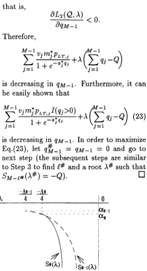
is decreasing in QM-1. Furthermore, it can be easily shown that

is decreasing in q M - 1 . In order to maximize Eq.(23), let q M V 1 = qM-1 = 0 and go to

next step (the subsequent steps are similar t o Step 3 t o find

e#

and a root A# such that

#

S M - ~ # ( A # ) = -&).

cl

* *

h 4 4 I n

- -

Figure 1. Functions of SM (A) and S M - 1 (A). Based on the above description, we propose an efficient and novel optimization algorithm (called Al- gorithm l ) to determine the optimal solution for the resource allocation Problem P 1 .

Algorithm 1:

Step 1.

Step 2. Step 3.

Rearrange the indices of Aj’s such that A1

2

A2

2 . .

. >

AM

2 AM+^

=

0 (here,

AM+^

=

0 is

a dummy variable). Let

e

= 0.

(let t# =

t) there exists

a unique root A# such that SM -e #( A # ) = -Q and the optimal solution Q# is

# -

j = 1 , 2 , . . . , M

-

e#;

otherwise, let Q , , , ~ - ~ + ~ -

q M - e + l = 0, set t +

e

+

I , and go to Step 3.

Cl

In general, such linearly constrained minimization problem can be solved by the successive quadratic programming method based on the iterative formulation and solution of quadratic programming subproblems

[ 1 6 ] . However, this method is complex. On the con-

trary, in Algorithm 1 the first

e#

-

1 iterations just do simple numerical comparisons. In the L#th iteration, since

SM-e#(A)

is decreasing in

A,

there must exist a unique root

A#

such that SM-e#(A#) = -Q

and hence the optimal solution

Q#

can be obtained. Note that A# can be easily obtained by simple numerical analysis. Therefore, Algorithm l is quite simple, efficient, and novel. By Lemma 1 it can be easily shown that this algorithm always converges in, a t worst, M-1 steps. The value of the objective function

given by Eq.(7) with the optimal solution

Q#

is

3.2.

sources

Minimizing the amount of testing re-

In this subsection, we consider another resource allocation problem. Assuming that the number of software faults still undetected in the whole system after the application of tl, t 2 ,

. .

.

,

t k is less than or equal t o

2. The project manager has t o allocate an appropri-

ate amount of testing resources to each module during the application of t k t o minimize the total amount of testing resources required throughout module testing From Eq.(6), this resource allocation problem [2-41.

(called Problem P 2 ) can be formulated as:

Min Eqj j = 1

q j 2 0 , j = l , 2

,...,

M .

Note th at from Eq.(25) we have

Th at is, it is impossible to reduce the number of software faults still undetected in the whole system to

E,”=,

v j m j r ( 1

-

p L T v , ) after the application of test in-

stance t k no matter which resource allocation method is used. This phenomenon is the limitation of the HGDM with logistic learning factor model.

(6)

Ignoring the constraint q j

2

0 and using the La-

grange method [15], Problem P2 is equivalent to find the minimum of

For convenience, we consider another problem (called Problem P2’):

Rilin c q j

j = 1

q j

2 0 ,

j = 1 , 2 , . . . , M .

Ignoring the constraint q j

2

0 and using the Lagrange

method [15], Problem P2’ is equivalent to find the minimum of

The necessary conditions B1-B3 for a minimum of E- q.(27) to exist are as follows [15]:

B2: X

>

0.

M

For Condition B1, from Eq.(27) we have

Aj Bj

= 1 - X = O , j = 1 , 2 , . . . , M(29) (1

+

B j ) 2

Since q j should be larger than or equal t o zero, we have 0

<

B3

5

1 for j = 1 , 2 , .

. . ,

M . Therefore, from

Eq.(29) we have X

>

0 (i.e., Condition B2 is satisfied) and

R 1

Since 0

<

B3

5

1, from Eq.(30) we can easily obtain (31)

4

X > - , j = l , 2 , . . . , 1

M.

4

and the root of Eq.(30) is

where Xj” = -l/(XAj). Therefore, we have

l j = 1 1 2 , . . . , M . (33) Let

(34)

where

By simple calculation, we have the following lemma. Lemma 2.

(i) r j ( X ) is decreasing in A; (ii) iim r j ( X ) = vjmj’(1

-

p L T , , ) ;

A-00

1

(iii) lim r j ( X ) = vjmj”(1 - -), where r j ( X ) is

- + 4 / ~ , ’PL,~,

given in Eq.(35). 0

Since X

2

4/Aj for j = 1 , 2 , . . . , M , for convenience

we rearrange the indices of Aj’s such that A1

2

A2

2

. . .

2

-4.?f. By Lemma 2 we have

M

C v j m ; ( 1 - PLT,,)

I

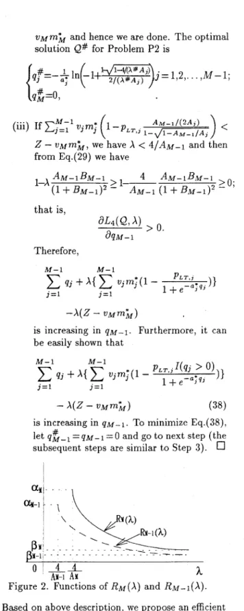
R M ( X ) _<

Since

RL(X)

=

CF.-1r3(X)

and r j ( X ) is decreasing

in A . RL(X) is decreasing in

X

for L = 1 , 2 , , M . Furthermore, from Eq.(35) we have y3(X)

>

0 for

all J , and from Eq.(36) RM(X) and R ~ . I - ~ ( X ) are M

(7)

constraint

xEl

.jmj.(l-p,T,,/(l+e-Q;q’)) =

z

(i.e., Condition B3) and based on Figure 2, the main steps

for finding the minimum of Problem P2 are depicted in the following:

Step 1 . Rearrange the indices of Ai’s such that A1

2

A2

2

. .

.

2

A M . Step 2. (i) (ii) (iii) Step 3. (i) ( i i ) If

xEl

v j m g ( 1 - p L T , , )

2

Z , it is impossible to reduce the number of still undetected software faults t o

Z

after the application of test instance t k .

If _{v j m j ” ( 1 -}_{p L T , ) )}

_<

_z

₅

exists a unique root A # (here, A#

2

4 / 4 4 )

such that R M ( A # ) = Z and hence we are done. The optimal solution &# for Problem P2 is

Since ( ( ~ 1 ~ 2 , . . . A M ) : ( q l , q z r . . . , Q M ) satisfies Eq.(25)} is the subset of { ( q l , q z , . . . , Q M ) :

( q l , 4 2 . .

. .

,

q M ) satisfies Eq.(26)} and q,#

>

0, j = 1 , 2 , .

. . ,

M , the optimal solution for Problem P2 is also

&#.

have

X

<

AM

and hence from Eq.(29) we

w M m h and hence we are done. The optimal

solution Q# for Problem P2 is

Z

-

u M m ; M , we have A

<

4 / A ~ - 1 and then from Eq.(29) we have

A M - 1 B M - 1 1-A (1

+

Bnci-1)’

-

th at is, 4 A M - I B M - I

>o;

>

1--

AM-^

(1

+

B M - I ) ~

-

a L 4 ( a A )

>

0. a q M - 1 Therefore,

-A(z

-

W M m h )

is increasing in q ~ - l . Furthermore, it can

be easily shown that

have

1 - X

is increasing in Q M - ~ . To minimize Eq.(38),

subsequent steps are similar t o Step let q M - l # 3).

0

= q ~ - l = O and go t o next step (the

A M B M

>

4 AMBM

>

o;

( 1

+

B . w ) 2

-

A M (1

+

B M ) ~

-

that is,

(37)

Therefore, I d 4 ( Q , A) is increasing in Q M .

Furthermore] it can be easily shown that

L3(Ql A) is also increasing in q ~To . minimize Ls(Q,A), let q$ = q~ = 0 and go to Step 3.

If

z!LL1

vjmj”(1 - p,,,,)

2 z

- v M m h , it

is impossible to reduce the number of stil- l undetected software faults to

Z

after the application of test instance t k .

a y j . . . . I RY-l(h) \ ! - . - . . - . . . - _ _ . 0

i 4 4

AY-i AY

h

Figure 2. Functions of R M ( A ) and R M - ~ ( X )

Based on above description, we propose an efficient and novel optimization algorithm (called Algorithm

2) to determine the optimal solution for the resource

allocation Problem P2.

If

I:!‘

u3m;(1

-

p,,,,)

<

z

-

v Mm b

I

.If - 1 A n f - 1 / ( ? A , ) Algorithm 2:

- P L T , J l - d l - A M - l / A J

there exists a unique root A # (here.

AM

>

Step 1. Rearrange the indices of ,4j’s such that A1

2

(8)

Step 2. Let t = 0 and

Z*

= 0.

Step 3. (i) If

E,"=;'

wjm;(1

-

p,,,,)

2 z

-

z,*

it is impossible to reduce the number of still undetected software faults t o

Z

after the application of test instance t k .

(ii) If

E;;'

v3mj+(l

-

p,,,,)

<

z

-

Z*

5 ,

(let- ting

e#

=

e)

there exists a unique root A# such that R M - ~ # ( X # ) =

Z

-

Z* and the optimal solution &# is

)

A M - ~ / 2.4

~ - P L T , ,

- j 1 -

otherwise, let qg-e+l - - y ~ - ' + l = 0 , set

go t o Step 3.

U

Z*

+ 2'

+

vM-em;M-e, set i! +-

e +

1, and In Algorithm 2 the first

t# -

1 iterations just do

simple numerical comparisons. In the t # t h iteration, since R M - [ # ( X ) is decreasing in A, there must exist a

unique root

A#

such that R M - e # ( X # ) =

Z

-

Z*

and hence the optimal solution Q# can be obtained. Note that

A#

can be easily obtained by simple numerical analysis. Similar to the discussion in Subsection 3.1, Algorithm 2 is, therefore, also quite simple, efficient, and novel. Furthermore, by Lemma 2 it can be easi- ly shown that this algorithm always converges in, at

worst, M - 1 steps. The value of the objective function given by Eq.(25) with the optimal solution Q# is

4. Relationship between Optimal, Average,

and Proportional Allocation Methods

In Section 3.1, we discuss the problem of optimal resource allocation if the total amount of testing resources for module testing is specified. In this section, based on the concepts of average allocation and proportional allocation, we introduce two simple resource allocation methods, the average allocation method and the proportzonal allocation method, respectively. Fur- thermore, we also investigate the relationship between these three allocation methods.

A resource allocation method is called an average allocation method if the testing resources are allocated to each module evenly. Let q j , a u g be the amount of testing resources allocated to module j during the application of t k by the average allocation method, and

then we have

Let Zavs be the number of still undetected faults in the whole system after the application of t k by the average allocation method, and then from Eq.(6) we have

A resource allocation method is called a proportion-

al allocation method if the amount of testing resources

allocated t o module j is proportional t o the number of still undetected faults in module j. Let qj,prop be the amount of testing resources allocated t o module j during the application of t k by the proportional allocation

method, and then we have Q j , p r o p

Note that if m; = mz =

. . .

= m t , the proportional allocation method is equivalent to the average allocation method. Let Zprop be the number of still unde-

tected faults in the whole system after the application of t k by the proportional allocation method, and then

from Eq.(6) we have

The optimal allocation method is said t o be bet-

ter than the average and the proportional methods

since Zopt

5

Z a u g and Zopt

5

Z p r o p . However, we

are also interested in how much better the optimal al- location method is. In the following, we investigate the value of Zopt/Zprop under the case pLT,j = pL, for

j = 1 , 2 ,

...,

M .

From Eqs.(24) and (43), we have

z o p t

d P L T ) =

-

ZProP

(44)

T ha t is, Zopt/Zprop is decreasing in p,,, which mean-

s that the larger the p,, is, the smaller the ratio of

the number of still undetected faults by the optimal allocation method t o that by the proportional method

(9)

is. In other words, as p , , increases, the optimal allocation method is much better than the proportional allocation method. Furthermore, since p , , represents the skill of detecting faults [la], from Eq.(44) the following can be observed: the better the skill of detecting faults, the better the optimal allocation method (compared with the proportional allocation method). By the same argument on Z o p t / Z p r o p , we have the

property that ZOPt/ZPrOP is decreasing in p , , . That is, the better the skill of detecting faults, the better the optimal allocation method (compared with the average allocation method).

5. Numerical Examples

Consider a software system consisting of 5 modules (i.e.,

A4

= 5). Suppose there are 4 test instances

t l 1 t 2 , t 3 , t 4 (i.e., k = 5) applied during module test-

ing so far. For each module, the parameters a j , b j , m j , and p,,,, , j = 1 , 2 , . .

.

, 5 can be estimated by using the software failure data, and then the estimated value of mj. can be obtained. The estimated val-

ues of m;, a j , b j , p L T S j and the weighting factor vj are assumed and listed in Table 1. Consequently, the total number of still undetected faults after the application of t l r t 2 , t 3 , t 4 is assumed to be 200 (since

E,”,,

m; = 200).

Example 1. Minimizing the total number of

undetected faults

Suppose the total amount of testing resources Q for module testing during the application of t s is 20k (i.e., 20,000) man-hours. The manager has t o allocate the

20k man-hours to the 5 modules to minimize the total

number of still undetected faults after the application of tj. Using the values of m;, a j , b j , P,,,~, and v j in

Table 1, the optimal solutions q: estimated by Algo- rithm l are shown in Table l. Consequently, the total number of still undetected software faults after the application of $ 5 estimated by Eq.(24) is Zopt = 115. Th a t is, the total number of still undetected faults is anticipated to be reduced from 200 to 115 by using the testing resources of 20k man-hours. T he reduction in the undetected software faults is about 42.5%.

Table 1. Allocated Testing Resources q,# for Minimizing undetected Software Faults.

( Q is assumed t o be 20k man-hours) Module m: a , b , a . - U , o* z , ~ ~~~ 1 50 0.02 0.1 1.0 1 12.79 3.6 2 45 0.08 0.2 0.6 1 5 . 1 7 19.2 3 40 0.2 1 0.3 1 1.76 28.3 4 35 0.8 5 0.03 1 0.28 34 5 30 1.0 10 0.003 1 0 30

Zopt =

E:=,

z3 = 115 (42.5% reduction)

Based on the average allocation method, from E- = qz,aug =

. . .

= q S , a v g = 4 and q.(40) we have

then from Eq.(41) we have Zaug = 128. Furthermore] based on the proportional allocation method, from E- q.(42) we have q 1 , p r o p = 5 , q 2 , p r o p = 4.5, Q 3 , p r o p = 4, ~ 4= 3.5, , and ~~ 5 , p r o p ~ = 3. Therefore] from Eq.(43) ~ ~

we have Zprop = 125. Obviously, the optimal allocation method is better than the proportional method and the average method. Furthermore, the optimal resource allocation method is very efficient in this example since the difference of Z p r o p

-

Zopt is significant.

In the following, consider the case p,,,, = p , , for

j = 1 , 2 , .

. .

,

5 and the estimated values of mj.

,

a j ,

b j and vj are also listed in Table 1. The curves

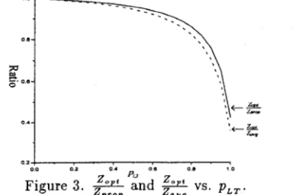
of Z o p t / Z p r o p and Z o p t / Z a v g vs. p , , are depict-

ed in Figure 3. As p , , = 0.1, from Figure 3 we

have Z o p t / Z p r o p = 0.995 and Zopt/Zaug = 0.993.

As p , , = 0.9, we have Z o p t l Z p r o p = 0.651 and Zopt/Zavg = 0.586. Obviously, if p , , is smaller, the differences of the number of still undetected software faults among these three resource allocation methods are less significant. Therefore, the average resource allocation method can be employed due to its simplic- ity if p , , is smaller. On the contrary, if p , , is larger, the optimal resource allocation method should be applied since it reduces the number of still undetected software faults much more significantly. In summary, both curves in Figure 3 are decreasing in p , , ; that is, the larger the p , , , the better the optimal allocation method (compared with the average and the proportional allocation methods).

0 0 0 1 0 . 0 - o m ( 0

..

PU

Figure 3. and vs. p , , .

P‘OP Z . * g

Figure 3 also indicates that the proportional allocation method is better than the average allocation method since

Zopt/Zprop

2.

Zopt/Zavg for 0

<

p , , 1. This result meets our intuition.

Example 2. Minimizing the total amount of

testing resources

Suppose the number of still undetected software faults after the application of t s needs to be reduced from 200 t o 120. The manager has to determine how

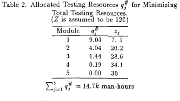
much testing resource is to be allocated for each module t o minimize the total amount of testing resources. Using the values of m;

,

a j

,

bj

,

p , ,

,

and v j in Table

(10)

1, the optimal solutions qf estimated by Algorithm 2 are shown in Table 2. Consequently, the total amoun- t of testing resources in module testing estimated by Eq.(39) is 14.7k man-hours. That is, the amount of testing resources spent during the application of t 5 is anticipated t o be 14.7k man-hours.

Table 2 . Allocated Testing Resources q: for Minimizing Total Testing Resources.

( Z is assumed to be 120) Module q: 2 3 1 9.03 7. 1 2 4.04 20.2 3 1.44 28.6 4 0.19 34.1 5 0.00 30 q: = 14.7k man-hours 6. Conclusions

In this paper, based on the HGDM with logistic learning factor, we investigate two optimal resource allocation problems in software module testing: 1) minimization of the number of software faults still undetected in the system after testing given the total amount of testing resources and 2) minimization of the total amount testing resources required given the number of software faults still undetected in the system after testing. Two efficient and novel optimization algorithms based on the concept of Lagrange multiplier method for the above two problems are proposed, respectively. In addition, the relationship between the optimal, average, and proportional resource allocation methods is investigated. Experimental results show that the optimal allocation methods are very efficien- t for solving the testing resource allocation problem. Furthermore, the results show that the better the skill of detecting faults, the better the optimal allocation met hod.

Acknowledgment.

We would like t o express

our gratitude for the support of the National Science Council, Taiwan, R.O.C., under Grants NSC85-2221- E002-015. Reviewers’ comments are also highly ap- preciated.

References

[l] M. V. Zelkowitz, “Perspectives of software engi- neering,” ACM Computang Surveys, Vol. 10, pp.

[a]

P. Kubat and H . S. Koch, “Managing test- procedures to achieve reliable software,” IEEE

Trans. o n Relaabalzty, Vol. 32, No. 3, pp. 299-303,

1983.

[3] H . Ohtera and S. Yamada, “Optimal allocation & control problems for software-testing resources,” 197-216, 1978.

I E E E Trans. on Reliability, Vol. 39, No. 2, pp.

[4] Y. W. Leung, “Software reliability growth model

with debugging efforts,” Microelectron. Reliab.,

[5] J. D. Musa, A. Iannino, and K. Qkumoto, Soft-

ware Reliability

-

Measurement, Prediction, Ap-

plication, McGraw-Hill, New York, 1987.

[6] M. Xie, Software Reliability Modeling, World Sci- entific Publishing Company, Singapore, 1991. [7] M. R. Lyu (ed.), Handbook of Software Reliability

Engineering, McGraw-Hill, New York, 1996.

[8] Y. Tohma, K. Tokunaga, S. Nagase, and Y. Mu- rata, “Structural approach to the estimation of the number of residual software faults based on the hyper-geometric distribution,” IEEE Trans.

on Software Engineering, vol. 15, No. 3, pp. 345-

355, March 1989.

[9] Y. Tohma, H. Yamano, M. Ohba, and R. Jaco- by, “The estimation of parameters of the hyper- geometric distribution and its application to the software reliability growth model,” IEEE Trans.

on Software Engineering, vol. SE-17, No. 5, pp.

483-489, May 1991.

[lo] R. Jacoby and Y. Tohma, “Parameter value computation by least square method and e- valuation of software availability and reliability at service-operation by the hyper-geometric distribution software reliability growth model (HGDM),” Proc. 13th Int. Conf. Software Engi-

neering, pp. 226-237, 1991.

[ l l ] T. Minohara and Y. Tohma, “Parameter estimation of hyper-geometric distribution software reliability growth model by genetic algorithms,”

Proc. 6th Int. Symposium on Software Reliability Engineering, pp. 324-329, 1995.

[12]

R.

H. Hou, S. Y. Kuo, and Y. P. Chang, “Ap- plying various learning curves to hyper-geometric distribution software reliability growth model,”

Proc. 5th Int. Symposium on Software Reliability

Engineering, pp. 7-16, 1994.

[13] R. H. Hou, S. Y. Kuo, and Y. P. Chang, “ Opti-

mal release times for software systems with sched- uled delivery time based on the HGDM

,”

IEEE

Trans. on Computers (accepted for publication).

[14] R. H. Hou, S. Y. Kuo, and Y. P. Chang, “Op- timal release policy for hyper-geometric distri- bution software reliability growth model,” I E E E

Trans. on Reliability (accepted for publication).

[15] M. S. Bazaraa and C. M. Shetty, Nonlinear Pro- gramming: Theory and Algoriihms, Wiley, New

York, 1993.

[16] M . J . D. Powell, A tolerant algorithm for linear-

l y constrained optimization calculations, DAMTP

Report NA17, University of Cambridge, England, 1988.

171-176, 1990.