Multivariable control of multi-zone chemical mechanical polishing

Multivariable Control of Multi-Zone Chemical Mechanical Polishing

Sheng-Jyh Shiul, Cheng-Ching Yu*', Shih-Haur Shen2, and An-Shih Su'

'Dept. of Chem. Eng., National Taiwan UniversitTaipei 106-17, TAIWAN 'Applied Materials Taiwan Ltd., Hsin-Chu 300, TAIWAN

Abstract - The modeling and multivariable control of the multi-zone CMP are studied in this work. In the process control notation, the manipulated variables are the three pressures applied to each zone. Therefore, this is a 60x3 non-square multivariable control problem. The singular value decomposition (SVD) is used to design a non-square

feedback controller. The proposed control system is test on

incoming wafer.s with different surface profiles. Results show that achievable performance can be maintained using theproposedSVD controller.

1. INTRODUCTION

Despite recent advances in CMP, some manufacturing concerns associated with successful implementation of CMP remain to he overcome. In theory, CMP can achieve global planarity, but there is still a problem that different operating conditions will result in non-uniformity in thickness of wafer surface. The within-wafer non- uniformity (WIWNU) indicates the variation in surface thickness across the wafer radial position, especially on thc

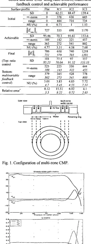
edge. Besides, the surface profile of wafers produced from electrochemical plating (ECP) process appears that the metallic layer is thicker on edge area. Thus, a new type of CMP, multi-zone CMP, offers an attractive alternative. Multi-zone CMP is expected to reduce WIWNU and to provide a wider processing window. Unlike the typical single zone configuration, the wafer carrier is divided into multiple zones in the radial position and different pressure can be applied to each zone (Fig. I). The objective of this work is to devise a systematic approach to the modeling and control of such CMP processes.

2. MULTI-ZONE CMP 2. I Process Description

Consider a CMP system where the wafer carrier is divided into three zones in the radial position and different pressure can be applied to each zone (Fig. 1). For a wafer camer with the radius of 150" (i.e., a 300 mm wafer), zone #1

covers 0-130mm, the second zone ranges fiom 130- 140mm, and third zone covers 140" and heyoud. Typically, the well-known Preston's equation [l] is used to model the polishing process. It describes the material removal as a linear function of pressure and rotation speed.

R R = K . p . v (1)

corresponding author; e-mail: ccvu@.ntu.edu.tw; f a : t886-2-

2362-3040

where K, is the Preston constant, p is pressure, and v is rotation speed. The Preston equation can be extended to multi-zone CMP in a straightforward manner. For the multi-zone system, the relationship between removal rate at the ith radial position and input variables can be expressed as:

RR, =

c

K P > , P, ' V (2)

where is the local Preston constant describing the effect of pressure from jth zone on the ith radial position,^, denotes the pressure of the jth zone, and v is again the rotation speed. Without loss of generality, assume that the rotation speed is fixed throughout all runs and vis absorbed into Kp,w for the subsequent development.

Copper (Cu) CMP is camed out on an Applied Materials' Reflexionm polisher using Titan ProfilerTM polishing heads. Polishing pad (Rodel ICIOIO) is used and the experimental copper CMP sluny is provided by Cabot Corporation. Electrochemical plating (ECP) process is employed for Cu plating. The 300" wafers without pattern are used in all tests. All copper thickness measurements are performed with an in situ i-Scan sensor. All the experiments were carried out according to a standard design of experiment procedure (DOE). The factors in this work are the three pressures applied to each zone and a pressure applied to the retaining ring. From center of the wafer to the edge, they are defined asp,, p2, p 3 , and prr, respectively. We devise two levels for each

factor such that a four-factor and two-level design of experiment (DOE) is camed out.

2.2 Steady-State Analysis

From the definitions of state and input variables, the steady-state behavior for the multivariable system can he written as follows:

x = K p . p (3)

where K, is the steady-state gain matrix. Given experimental data, K, matrix ( E W " ~ ~ ) can be determined from the least square regression. The regression result versus position on wafer is given in Fig. 2a.

Let us use the singular value decomposition (SVD) to analyze the system. The SVD decomposes the K, matrix of model into three matrices:

K p = UXV'

(4) where

U

is a orthonormal matrix ( S W ~ ~ ~ ) in the output side, V is the input orthonormal matrix and

X

is a

3x3 diagonal matrix with the singular value (ui) as the diagonal element. The ratio of the largest singular value to the smallest is the condition number (x=u,,,Jumjn) which is a quantitative indicator of closeness to singularity. After proceeding SVD, the V matrix is found similar to identity. Then each column of

U

matrix is plotted against position on wafer (Fig. 2b). As can be seen in the figure, the trends of the three columns in

U

matrix are quite similar to those of K, matrix. It indicates that the three directions are just enough to describe the characteristic of multi-zone system. The singular values sorted by number are 264, 3 1, and 16, respectively, and condition number (K) is 16, i.e., quite far away from a singular system. Thus, this is a well-defined multivariable system with 60 states and 3 inputs.

Because of the characteristic of a non-square property of system, it is not possible to keep all 60 outputs at their set points using only 3 inputs. Thus, non-unifomiity is an inherent property of this multi-zone CMP. Given the initial surface profile

bo)

(measured) and the desired thicknessy”, the amount needs to be removed (Ay“) can easily calculated by

After the CMP with a polish time of At, the error between the desired and actual thicknesses can he expressed as

Ayd = y o - y d ( 5 )

E

= y - y d = (yo - y“)-(yo - y)

(6) = (x” - x) .At

Eq. (6) also indicates that the error is due to difference of actual removal rate (x) and desired removal rate (xd). In terms of the removal rate, we have:

x d = K ‘ p ( 7 )

Solving Eq. ( 7 ) by the least-square method, the input pressures are computed:

= (K: K$K: . x d = K: .xi ₍₈₎ where the superscript

t

denotes the pseudo-inverse. Substituting p into Eq. ( 3 ) , one finally obtains:

Em,”

= ( I - K , K : ) x d . A t

(9) = (I - K ~ K:

AY^

The above equation indicates the achievable performance for this multi-zone CMP and it is characterized by the deviation of the projection matrix ( K-K: ) from an identity matrix. Consider the case when every entry of the vector Ay“ takes the value of 1. Fig. 3 shows the shape of the surface profile in the radial position. Since the 2-nom

of Emi,

is equal to 0.0735, it implies an averaged error of 73.5.A for l000.A removed.

3. CONTROL

In the process control notation, the measured data are the controlled variables and the manipulated variables are the three pressures applied to each zone. Therefore, this is a 60x3 multivariable control problem. The control objective is to maintain uniform surface profile using all three manipulated variables. Because this is a non-square system,

it is not possible to keep all the outputs at their set points using only 3 inputs. A 2-norm-based objective function is then considered:

where J is the objective function,

y’

and y”are vectors (E%~’“’) of measured thicknesses (at end of each run, i.e., y’=y(tf)) and the desired thicknesses, respectively.

Some performance indices are introduced here.

J =

I~Y’

-

~‘11,

(10)

i) Standard deviation (SD):

ii) m-norm ofthe deviation between measured thickness and the mean:

m-norm = ljy’

-y’llm

(12)

iii) The range of measured thickness:

(13)

/ I

range = ym- - ymxS iv) Non-uniformity (NU):

Those provide simple measures of quality after polishing. Obviously, the achievable performance defined by Eq. (9) also provides an absolute hasis to evaluate control performance.

3.1 Ratio Control

Since the process model, at least Kp, is perfectly know, a simple control strategy can be implemented for the multi- zone CMP process. It is a feedforward control where the ratios of the pressures are computed from the model inverse and ratios are maintained throughout the run.. The final NU in flat case is about 5% which is acceptable in the fabrication. In other cases, the first two surface profiles with small SD value, IC1 and IC2, are regarded as

finer initial conditions among the three. The indices of final status of those cases are slightly more than those of achievable status. However, their NUS are both kept within

5%. The SD of final status of IC3 is reduced while the other indices are not changing much. Basically, this kind of initial surface profile is hard to handle for the system. Thus, that indicates that ECP is supported to prevent production of that profile.

3.2 Multivariable Feedback Confrol

It is based on concept of feedback control. The controller adjusts the pressure input simultaneously according to the deviation between measured thickness by sensor and set points (desired thickness). To monitor the change of surface in a polish run, therefore, an in situ sensor

is

required to measure copper thickness on-line and a non- square feedback controller necessary to generate input pressures. Fig. 4a shows the non-square system with the tall process (more output than inputs) and a fat controller (more input to the controller than the control output). The

SVD-based approach is employed to design the inversed- based controller. First, the steady-state gain matrix is decomposed into three matrices and the multivanable system can be expressed as (Fig. 4b):

1 1 Y = - K o . D . p = - ( U Z V r ) D . p S (15) S U S = U .diug[-] . V T . D . p

Next, the derivative part of the controller is taken as the inverse of D and the output of the PI part of the controller becomes:

P = D-'p,, (16)

Thus, the relationship between the ppI and Y becomes:

Multiply the both sides with UT matrix (recall that both U and V are orthonormal matrices, i.e., UU' = I and

V'V = I ), one obtains:

S

UTY and VTppl correspond to the output and input in the principle directions and they are defined as Y' ( E % ' ~ ' ) and p'(~%"'), respectively. Therefore, we are left with a decoupled square system with simple diagonal elements,

cr, / s , Define the diagonal matrix as Gp*, the multivariable

system becomes:

Y' = G;p' (19)

Fig. 4c also shows the result of transformation. Note the diagonalizing effort is absorbed into the controller as shown in Fig. 4b. Therefore, standard multivariable control method can be applied to this decoupled square system. Taking the flat profile as an example, Fig. Sa shows the snapshots of the surface profiles throughout the polishing process. The control performance can be seen from the responses of the manipulated variables (Fig. 5 b & c) and the tracking error (Fig. 5d). In terms of the principle output (Fig. 5d) and input (Fig. Sc), the output settles to the set point in less than 20 seconds and acceptable control performance is obtained using the SVD-based multivariable controller. For CMP process, the ultimate performance measure in the uniformity. Table 1

summarizes all the indices using the ratio control as well as the multivariable feedback control. Comparison is made with respect to the achievable performance (Table I).

Results clearly indicate that the multivariable feedback control leads to the performance close to the achievable performance while the ratio control shows 4-15% deviations from the achievable one. More importantly, the seemingly complex control system can he design systematic manner with rather standard feedback design methodology.

4. CONCLUSION

In this work, a systematic modeling and control system design approaches are proposed for a multi-zone CMP system, The multi-zone CMP is intended to reduce the within-wafer non-uniformity (WIWNU) by manipulating different pressures across the radial position. This leads to a non-square multivariable system, a 60x3 system for the example studied. In the modeling phase, two 23 full factorial experimental design is carried out and steady-state gain matrix is obtained from the lease square regression followed by including the dynamic element associated with each input. For multivariable control, two control strategies with different degrees of complexity are proposed. First, a simple ratio control is designed based on the pseudo- inverse of the process model and, provided with the initial surface profile, the input pressures are computed and the ratios are maintained throughout the polishing run. The results show that, while giving reasonable uniformity, the performance is a little short from the achievable performance. Next, an on-line multivanable control system

is designed. The singular value decomposition (SVD) is used to project the input and output in the principle directions and, therefore, the controllers can be designed in a reduced dimension (3x3) for a decoupled system. Then, the diagonal controllers are transformed back to the true inputloutput spaces. This significantly reduces the engineering effort in control system design. Results show that achievable control performance can he maintained using the SVD-based multivariable controllers.

.

ACKNOWLEDGEMENT

SJS, AJS and CCY thank National Science Council of Taiwan for the financial support under the grant NSC 92- 22 14-E002-032.

REFERENCES

[I] Preston, F. W., "The theory and design of plate glass polishing machines",

J

Soc. Glass Technology, I 1, 214-256 (1927).

Table 1. Different uniformity measures of wafer surfaces before and after CMP using ratio control, multivariable

feedback control and achievable performance

Surface protile Flat IC1 IC2 IC3

--norm 0 378 636 603 0 444 714 734 NU (?4) 0 0.71 I 1.15 \\E

11

727 535 698 1170 SD 0 62.21 88.47 159.4 Initial range I, "112 SD 95.46 70.3 91.61 153.6 --norm 189 142 321 457 range 363 272 541 802 NU(%) 4.77 3.51 4.58 7.68 7x6 . . . 61x . . 740 . . . i > i x 7(1 570 703 1201 97 157 1.52 353.33 123 225 330 444 189 143 322 455 379 345 528 778 362 273 541 800 ..83 7.72 - - n o m Bottom: multivariable range feedbock . .. . .~ '.55 7.53 i.02 4.1 ".__ J.72 2.65

0'

Fig. 1. Configuration of multi-zone CMP

etesd".**-lD as," msmr

10

J(D1

10

Fig. 2. Steady-state gain vectors and vectors of the U matrix from SVD -0 03 -0 c4 _{0 0 7 3 5} 5 0 1m 1m 0 oso PD.,tlO" -tsr

<",

Fig. 3. The error vector of achievable performance by assuming input vector of unity.

(a) Original non-square system

I I

(b) SVD of the Process and Controller

(c) Equivalent Decoupled System

Fig. 4. Evolution of the SVD-based design and corresponding block diagrams.

.L

_.

- I. -7-w I& Im

'

0 _1--11 (a) (b)

[LT

i

T

4

:il

:I

_--

~."--

'7

.,::dm

,~~ 7 " m u P (C) ( 4

Fig. 5 . Results of multivariable feedback control for incoming wafer with flat profile: (a) snap shots of surface profile, (b) pressures, (c) principal input, and (d) error in the principle direction.