國
立
交
通
大
學
資訊工程系
碩
士
論
文
以機率和圖論分析行動學習之學習模型
An Efficient Learning Model for Mobile
Environments using Graph and Probability
Analysis
研 究 生:于立杰
指導教授:陳登吉 教授
以機率和圖論分析行動學習之學習模型
An Efficient Learning Model for Mobile
Environments using Graph and Probability
Analysis
研 究 生:于立杰 Student:Li-Chieh Yu
指導教授:陳登吉 教授 Advisor:Deng-Jyi Chen
國 立 交 通 大 學
資 訊 工 程 系
碩 士 論 文
A ThesisSubmitted to Department of Computer Science and Information Engineering
College of Electrical Engineering and Computer Science
National Chiao Tung University
in partial Fulfillment of the Requirements
for the Degree of
Master
in
Computer Science and Information Engineering June 2004
中華民國九十三年六月
國 立 交 通 大 學
論 文 口 試 委 員 會 審 定 書
本校
資訊工程系 碩士班
于立杰
君
所提論文:
以機率和圖論分析行動學習之學習模型
An Efficient Learning Model for Mobile
Environments using Graph and
Probability Analysis
合於碩士資格水準、業經本委員會評審認可。
口試委員:
指導教授:
系主任:
中 華 民 國 九十三 年 月 日
博碩士論文授權書
本授權書所授權之論文為本人在 國立交通大學 資訊工程 系所 93 學年度 第 2 學期 取得 碩士 學位之論文。
論文名稱:An Efficient Learning Model for Mobile Environments using Graph and Probability Analysis 指導教授:陳登吉 教授 1.□ 本 技 各 本 一 2.□ 本 國 及 重 本 一 3.□ 本 統 之 以 文 下 本 校 上 授 本 研 ( 日 同意 □不同意 人具有著作財產權之上列論文全文(含摘要)資料,授予行政院國家科學委員會科學 術資料中心(或改制後之機構),得不限地域、時間與次數以微縮、光碟或數位化等 種方式重製後散布發行或上載網路。 論文為本人向經濟部智慧財產局申請專利(未申請者本條款請不予理會)的附件之 ,申請文號為:______________,註明文號者請將全文資料延後半年再公開。 同意 □不同意 人具有著作財產權之上列論文全文(含摘要)資料,授予教育部指定送繳之圖書館及 立交通大學圖書館,基於推動讀者間「資源共享、互惠合作」之理念,與回饋社會 學術研究之目的,教育部指定送繳之圖書館及國立交通大學圖書館得以紙本收錄、 製與利用;於著作權法合理使用範圍內,不限地域與時間,讀者得進行閱覽或列印。 論文為本人向經濟部智慧財產局申請專利(未申請者本條款請不予理會)的附件之 ,申請文號為:______________,註明文號者請將全文資料延後半年再公開。 同意 □不同意 人具有著作財產權之上列論文全文(含摘要),授予國立交通大學與台灣聯合大學系 圖書館,基於推動讀者間「資源共享、互惠合作」之理念,與回饋社會及學術研究 目的,國立交通大學圖書館及台灣聯合大學系統圖書館得不限地域、時間與次數, 微縮、光碟或其他各種數位化方式將上列論文重製,並得將數位化之上列論文及論 電子檔以上載網路方式,於著作權法合理使用範圍內,讀者得進行線上檢索、閱覽、 載或列印。論文全文上載網路公開之範圍及時間 – 校及台灣聯合大學系統區域網路: 年 月 日公開 外網際網路: 年 月 日公開 述授權內容均無須訂立讓與及授權契約書。依本授權之發行權為非專屬性發行權利。依本 權所為之收錄、重製、發行及學術研發利用均為無償。上述同意與不同意之欄位若未鉤選, 人同意視同授權。 究生簽名: 學號:9117549 親筆正楷) (務必填寫) 期:民國 年 月 日
國家圖書館博碩士論文電子檔案上網授權書
本授權書所授權之論文為本人在國立交通大學資訊工程系所 93 學年度第 2 學期取得碩士學位之論文。
論文名稱:An Efficient Learning Model for Mobile Environments using Graph and Probability Analysis 指導教授:陳登吉 教授 □同意 □不同意 本人具有著作財產權之上列論文全文(含摘要),以非專屬、無償授權國家圖書 館,不限地域、時間與次數,以微縮、光碟或其他各種數位化方式將上列論文 重製,並得將數位化之上列論文及論文電子檔以上載網路方式,提供讀者基於 個人非營利性質之線上檢索、閱覽、下載或列印。 上述授權內容均無須訂立讓與及授權契約書。依本授權之發行權為非專屬性發 行權利。依本授權所為之收錄、重製、發行及學術研發利用均為無償。上述同 意與不同意之欄位若未鉤選,本人同意視同授權。 研究生簽名: 學號:9117549 (親筆正楷) (務必填寫) 日期:民國 年 月 日 1. 本授權書請以黑筆撰寫,並列印二份,其中一份影印裝訂於附錄三 之一(博碩士論文授權書)之次頁﹔另一份於辦理離校時繳交給系所 助理,由圖書館彙總寄交國家圖書館。
以機率和圖論分析行動學習之學習模型
學生:于立杰 指導教授:陳登吉 博士
國立交通大學資訊工程系所碩士班
摘要
無線網路及行動裝置已普遍商業化,這些硬體使得數位學習一日千里。像 video-phone 和 Multimedia-on-demand 這些應用也使得多體在這個領域更有發 展。 目前還有許多在行動學習上的研究像 Location Management、QoS 等,在此環境 中資料分散在不同處,我們的研究是找出一個放出一個放置資料的方來提升存取 的成功率,同時使用 moving pattern 來改善資料放置的效能。假設學生要存取 不同課程,我們會根據目前的網路狀態定一個成功的機率,同時安排課程也是一 個議題,如何在有效的時間內來學習是一項挑戰。這在這篇論文裡,我們用 moving pattern 和 data allocation 來改善在行動 學習環境下的存取效能。在課程安排的方法裡會提供學習路徑以及如何在時間內 學完,在我們提出的方法中會用實體和邏輯上兩種角度來看,實體面主要探討存 取成功率,而邏輯面探討課程安排。
最後我們會一些例子來看這方法的效能如何,也會在不同的網路型態下來研 究應用
An Efficient Learning Model for Mobile
Environments using Graph and Probability
Analysis
Student: Li-Chieh Yu Advisor:Deng-Jyi Chen
Department of Computer Science and
Information Engineering
National Chiao Tung University
Abstract
Wireless networks, handheld and wearable devices, and devices to sense and control appliances are now a commercial reality. Significant hardware progress in recent years has stimulated the ubiquitous e-learning environment. Applications such as video phones, multimedia-on-demand, and so forth will create new opportunities to access multimedia-rich information in mobile learning environments.
There are many areas currently under investigation in mobile learning environments, such as location management, quality of service, and bandwidth management, to name a few. In mobile environments, data (educational curriculums in multimedia form) is usually distributed disparately across several sites. An interesting concept is modeling such an environment to find a way to allocate courseware (or educational curriculums in multimedia form) such that the probability for successful
learning of the required courseware unit based on the learner's learning behavior can be obtained. Assuming that learners need to access different curriculums from remote sites within the network environment, we can define the probability that the needed courseware unit be accessed and learned successfully based on all connected local and remote sites by determining all possible routing paths. In addition, arranging a suitable learning sequence for the learner is an important issue. We also consider time restrictions by helping learners meet the imposed time restrictions presents an additional challenge.
In this thesis, we incorporate the concept of moving patterns and data allocation scheme to improve the probability of the required courseware unit that can be accessed and learned successfully over a mobile environment. A course planning scheme to suggest a learning sequence and to consider the time constrain problem is addressed. Specifically, the proposed approach uses two views in modeling: the physical view and the logical view. In the physical view, we consider and model the link reliability (communication links), Multi-access Probability (the access problems), moving patterns (user's learning behavior), and data allocations (location management) in the mobile learning environment. In the logical view, we consider and model the course planning strategy to find the suitable way for a learner to learn a particular courseware unit. Numerical examples are given to enumerate the proposed approach. Several simulation results based different topologies are studied to illustrate the applicability of the proposed approach.
ACKNOWLEDGEMENTS
First and foremost, I gratefully acknowledge my advisors, Dr. Deng Jyi Chen. I have received invaluable assistance and innumerable suggestions from him, especially during the academic year while I am in scholar in the Department of Computer Science and Information Engineering at University of National Chiao Tung University in Taiwan. He has spent enormous amount of time and effort to enhance my ability in research. I wish there were a better word than thanks to express my appreciation to Dr.Chen. Because of his long time advice, I have learned much not only in academic research but also in practical applications. His thoughtful insights and generous patience have contributed greatly to this thesis. I have received much assistance from my advisor, and for this I am extremely thankful. Acknowledgements are due, first, to my advisor, my parents, and my friends for encouragement, understanding, and infinite patience, especially during the year in school. I also wish to thank my friends in Lab for their continuous encouragement and sincere help. In addition, special appreciation is due to my advisor for his encouragement and research supports. Finally, my deep gratitude goes to my parents, who have given so much help to my life, and who are always there while times are difficult. To them I dedicate this thesis.
Table of contents
Chapter 1...1 1.1 Mobile Learning ...1 1.2 Problem Statement ...3 1.3 Research Methodology ...3 1.4 Thesis Organization ...4 Chapter 2...5 2.1 Area Overview...5 Chapter 3...8 3.1 Introduction ...8 3.2: Assumptions ...10 3.3 Notations ... 11 3.4: Link probability ... 11 3.5: Multi-access Probability ...12 3.6: Moving patterns ...13 3.7: Data allocation ...15 Chapter 4...174.1 The Learning sequence Environments ...17
4.2 Notations ...20
4.3 Assumptions and goals of course planning ...20
4.4. Minimum Weight Branching ...21
4.5 Using data allocation to allocate courseware unit in the physical network and compute the probability ...24
4.7 The Time restricted problem ...31
Chapter 5...39
ARPA network: ...39
Pacific Basin network: ...42
TANet topology: ...45
3-Cube network: ...48
List of figures
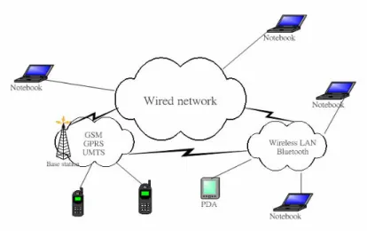
Figure 1: Network architecture of multimedia mobile learning system……2
Figure 2: Application scenario………9
Figure 3: Mesh network………10
Figure 4: Ad hoc networks………10
Figure 5: Mobility patterns………13
Figure 6: RMAP pattern………14
Figure 7: DMDB network………15
Figure 8: Tree structure of media………16
Figure 9: The Capability Indicator structure………18
Figure 10: Map the course to physical network ………20
Figure 11 Idea of learning path ………21
Figure 12: Relationship of courseware unit ………23
Figure 13: Branching of the relations………23
Figure 14 course relation and physical network topology………26
Figure 15: Branching of physical network topology………26
Figure 16: Data allocation tree for mesh physical network………27
Figure 17:A simple Mesh connected network………27
Figure 18: Successful probability ………28
Figure 19: Course Difficult………28
Figure 20: Data Base of examination………29
Figure 21: course distribution………30
Figure 22: Results of the quiz paper………31
F i g u r e 2 3 : L e a r n i n g c u r v e … … … 3 3 Figure 24: Relations of the courseware unit………33
Figure 25: Find the branching………35
Figure 26: Score percentage………35
Figure 27: course relation………35
F i g u r e 2 8 … … … 3 6 Figure 29: Result learning path………37
Figure 30: Learning paths………39
Figure 31: ARPA network………40
Figure 32: Allocation of ARPA network………40
Figure 33: Pacific Basin network………43
Figure 34: Allocation tree for Pacific Basin network………43
Figure 35: TANet topology………46
Figure 37: 3-Cube network………49 Figure 38: Allocation of 3-cube network………49
List of tables
Table 1: Link probability………12
Table 2: Moving frequency matrix………13
Table 3: Transition Probability Matrix………14
Table 4: A math program example………19
Table 5: The courseware unit………33
Table 6: Simulation result of APRA network………42
Table 7: simulation result of Pacific Basin network………45
Table 8: Simulation of TANet………48
Chapter 1
Introduction
In this chapter, we introduce an overview to the research area, the advent of mobile e-learning and discuss some of the important impacts of mobile e-learning. Based on the potential for e-learning, we formulate a problem statement that proposes the enhancement strategies for mobile e-learners. This chapter concludes with a discussion of the research methodology and the organization of the thesis.
1.1 Mobile Learning
In general, learning involves learning the things that we do not understand. In the knowledge exploding modern society, we find that learning is not merely restricted to the classroom, but technology has enabled us to extend beyond classroom boundaries. Besides traditional face-to-face teaching, the introduction of networks, both wired and wireless, has enabled new forms or channels for learning such as remote learning and e-learning.
Recently, wireless networks have become extremely popular, with access points becoming available at phenomenal rates. Mobile users are now able to demand access to content almost anywhere they want. The recent proliferation of mobile devices has increased such demand. These mobile devices (such as mobile phones and PDAs) are becoming increasingly powerful enough to handle multimedia data. Wireless networks such as GPRS and GSM are also beginning to support higher transmission rates, thus making them ideal mediums for multimedia data transmission. GSM supports wireless voice and digital services. GPRS supports non-voice services over cellular networks. Both networks come with rich features for such services and applications making them potential distribution mediums for multimedia services such as voice, video, multimedia on demand, video conferencing and mobile Internet, supporting data rates of up to 2mbps [5].
Technology in recent years has contributed much to the rise of e-learning and the introduction of new forms of teaching and learning.
The use of multimedia and the introduction of high-speed networks have only enhanced e-learning channels. The recent popularization of wireless networks and the proliferation of mobile devices have extended the possibility of e-learning to users of mobile devices, thus creating several opportunities for investigation in this area.
The potential mobile users create several opportunities for mobile e-learning. While mobile e-learning is not new and has been in practice in the US defense for many years, it has been proved to be the most efficient and most economical cost learning patterns. There are several governmental organizations implementing similar strategies. The potential for mobile e-learning will be extremely vast once the underlying infrastructure can unleash its potential. Access to information immediately and on-demand will be an evermore important requirement for users of mobile devices. This also applies to the mobile e-learning arena.
Mobile e-learning will not exist in isolation, but can cooperate with other technology such as establishing a knowledge base, digital learning materials and learning strategies.
In Figure 1, we show the network architecture of a multimedia mobile e-learning system and how the system relates to the wireless network as a whole. In this diagram, each mobile device can communicate through the wired or wireless link.
Mobile e-learning is not just a form that only provides mobile learners the sequential readable content, but also it should be an interactive communication between the instructors and learners [5]. Thus, courseware materials required by learners or instructors can also be provided in advance. In a simple example, learning activities in a museum visiting can be relied on the time and where visitors (learners) are located, the route they have taken, and what they have already seen so far.
There are several areas in mobile e-learning to be explored. Among these, include usability, security, performance and so forth. How to make a great performance for a suggested learning strategy and use a good data allocation scheme to make the accessing courseware unit smoother is an important issue to that we take into account.
1.2 Problem Statement
This study is to propose a scheme to improve Mobile-Learning by using a structured graph to model the different wireless networks and use a courseware planning scheme to spare the learner’s time by suggesting a learning sequence.
Specifically, we
z Investigate the standard which the Mobile-Learning follows and the challenges of Mobile-learning.
z Investigate and study related research on improving mobile-learning by sparing learner's time to meet the required grades. We also study other schemes related to improving the probability to obtain courseware unit.
z Propose a scheme for mobile e-learning to make the successful access probability better and suggest a learning sequence of each kind of learner.
z Extend the model to consider the time constraints of learners.
In this research, we investigate the use of the Link Probability to model the reliability of a communication link in the network. Multi-access Probability is used to formulate the probability of a courseware unit required by a learner through every possible routing path. Moving Patterns and the Data allocation scheme is used to improve the Multi-access Probability. Branching is used to suggest a learning sequence for the learner to spare the time. With the time constraint, we modify the model to meet the requirements.
We conduct a quantitative evaluation of the proposed model by demonstrating its applicability with experiments and examples.
1.4 Thesis Organization
In Chapter 2, we review previous related work, including Location Management, Moving Patterns, the Link Reliability aggression model, and Multi-access Probability. Chapter 3 thoroughly describes the Physical view and the algorithm needed to evaluate the probability of probability to obtain the courseware unit required by learners. The scheme that formulates communication links and better arrangements based on moving patterns is presented in this chapter. In Chapter 4, we present the steps of Branching, and coursing planning scheme. In chapter 5, we present some examples and simulation results that demonstrate the effectiveness of the proposed method. Finally, Chapter 6 states conclusions and future work.
Chapter 2
Related Work
In this chapter, we discuss related research and present an overview of these models discussing their similarities, differences, advantages and disadvantages. We also take a look at their applied environments.
2.1 Area Overview
Several related research work [22] discusses the architecture of mobile-learning environments. The architecture of mobile learning environments is concerned with the development of the standards, and providing interoperability among heterogeneous systems and learning object reuse. Based on the standardization work, they propose open and distributed architectures that identify some common services (e.g. software service) for e-learning domains.
Some mobile learning architecture has also integrated digital content topics in hybrid learning environments [23]. These research projects are concerned about digital representation such as three dimensional graphics and advanced animation techniques. They conduct analysis on the possibility of content that might be able to imitate or to substitute the teachers' human existence itself.
Other related works focus their efforts on e-learning theories. Like constructivist values for web-based instruction [15, 16]. In these research projects, their attempts are focused on trying to do convert traditional (face-to-face) courses to multimedia web-based courses. They focus on ways to encourage interactive learning and the use of
motivational strategies. In their experiments, they train students using digital course and video tapes of an instructor answering questions and discussing course content. In another theory, role-base learning theory, they focus on familiarizing students with intellectual frameworks and establishing principles and general approaches. Lastly, there is research that focuses on best approaches to developing educational tools and methods that deliver the principles and teach content material.
The research areas in e-learning and mobile learning are endless, and sometimes extend beyond. We look at some relevant research in the area
of course planning and discuss these in detail.
Related Researches
z Data Allocation Scheme by Incremental Mining of Moving Patterns[24] In this paper, the authors propose a data mining algorithm that involves mining user moving patterns in a mobile computing environment and exploiting the mining results to develop data allocation schemes so as to improve the overall performance of a mobile system. In this project, they consider both personal and shared data. Personal data are those only accessible by each individual data owner. Shared data are those accessible by a group of users. Their research considers the data allocation scheme but does not focus particularly on Mobile-Learning.
z Mobile Learning: New Paradigm in E-learning[25]
In this paper, the authors propose four functional levels. 1. Mobile-Learning application. 2. Mobile user infrastructures. 3. Mobile protocols. 4. and Mobile network infrastructures. These are used for simplify the design of system. It also discusses knowledge management and learning communities. Knowledge management considers learning as dynamic, and places emphasis on content that is new. The authors suggest on-line experts and best sources. However, they do not consider time restricted students and how these students could go about achieving their requirements.
z The Delay-Constrained Minimum Spanning Tree[26]
In this research, the authors formulated the problem of constructing broadcast trees for real-time traffic with delay constraints in networks. They discuss attempts to solving network problems, not related to the e-learning area, but presents ideas that can be applied to e-learning strategies. The focus of this research is on directed networks and using an efficient heuristic method to solve the problem for the unconstrained minimum spanning tree problem. This indicates the fastest delay-constrained minimum tree in a heuristic way and is more efficient than other constrained minimum trees, because others [21] were found to be much slower than this method.
Conclusion
In the previous researches [17, 18], there is much emphasis on learning strategies but they do not mention the performance related to accessing material. In the Data allocation scheme [19], most of them did not discuss moving patterns as a method of improving performance. Other learning strategies are discussed the view point of education but not on course planning in particular. We will discuss these schemes in chapter 3 and chapter 4 in greater detail.
Chapter 3
Physical view
3.1 Introduction
In Related Works, we mentioned what problems we want to solve in the research. We basically divided them into two areas. Area one is Physical view. The Physical view is the first part of the focus of this research and is concerned with network reliability. This is an important consideration when allocating resources in such an environment. In this chapter we discuss the physical aspects of wireless networks such as 3G networks and discuss the important properties related to mobile learning such as link probability, Multi-access Probability, moving patterns and data allocation.
There are many research topics involved in the study of mobile networks. For example, consider a mobile phone. It is easy to explain a mobile learning infrastructure with mobile phones, because many of us have experience with them. Mobile phones existed for a single purpose, to be able to make phone calls to anywhere from anywhere. However, recently, mobile phones have become increasingly sophisticated with several enhancements, including built-in organizers. Within time, mobile phones will be able to fetch courseware unit from the Internet, enhancing our vision of mobile learning.
Consider commuting from one city to another, for example, Taipei to Kaohsiung. Suppose the shortest possible path from Taipei to Kaohsiung is currently congested with traffic. You could use a mobile device to retrieve information immediately about finding the next quickest route and avoid traffic congestion. This example reinforces the potential for mobile learning. Such applications can provide better service quality and enhance our daily lives. Figure 2 shows the benefit of learning information immediately.
Figure 2: Application scenario
3G mobile networks offer true potential for multimedia over wireless networks. While the hype of 3G failed to materialize, there are still several opportunities for the implementation of such networks in the future. Some features of 3G mobile environments include:
Mobile Multimedia networks facilitate the ubiquitous services of multimedia applications for mobile users independent of time and location. One of the challenging problems facing the system is location management. In cellular network architecture, the geographic area is divided into adjacent cells, each covered by a base station. Several base stations are grouped together to form a Location Area (LA).
All base stations in an LA are connected to a Mobile Switching Center (MSC) using land links. The MSC acts as an interface between the wireless network and the Public Switched Telephone Network (PSTN). However, by equipping Base Station Subsystems (BSS) with distributed switches, two mobile hosts can directly communicate with each other without a PSTN connection.
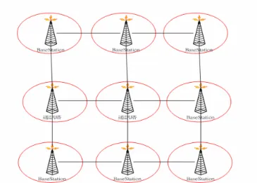
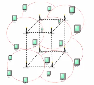
Figure 3 and Figure 4 are the possible examples of the applied environments.
Figure 3: Three cube network
Figure 4: Ad hoc networks
3.2: Assumptions
Once we have understood and defined the possible applied environment, we formulate the basic assumptions for the model below to be used throughout this thesis.
Given:
-Directed graph topology -Difficulty of each edge
-Hit Ratio of each courseware unit
-Branches Goals:
-Find all specific learning paths that meet the goals of each student.
3.3 Notations
G(V,E) is the directed graph in which V represents the nodes set of processing elements and E represents the edge set of course relation under consideration a node i in v.
Pr(Si|ti|tmax) is the result of a request sent by a user, the
material in order provider may need to send several resources back P(useri) is ordered sequence reliability for medium Si.
Dij is the difficulty for a user to finish a course between
course i and course j
HRi is the Hit Ratio of courseware unit i
Path(i) is the path that User i needs to take to finish the entire course
Ef(i) is the efficiency of course i after transformed into an Efficiency function.
RMAP(U): Remote Media Access Probability for a single mobile user
PR(ei ,r):The probability of the link ei can work well at
traffic ratio r (r=traffic load/link capacity).
TR(ei):The initial transfer reliability of link at traffic load=0.
3.4: Link probability
Link probability deals with the quantization of communication links to determine network reliability. In link probability, the initial transfer reliability is formulated and from this, a simple linear
regression model is used to get the approximate dynamic probability. TR(ei):The initial transfer reliability of link at traffic load=0.
PR(ei,r):The probability of the link ei can work well at traffic ratio r (r=traffic load/link capacity).
PR(ei,r)=(B0+B1*r)*TR(ei)…………B0 and B1 are shown in the table bellow
Table 1: Link probability
Ratio 0.0~0.2 0.2~0.4 0.4~0.6 0.6~0.8 0.8~1.0
B0 B1 B0 B1 B0 B1 B0 B1 B0 B1 Coef.
1.23 -1.17 1.28 -1.08 1.35 -1.01 1.43 -0.96 1.50 -0.89
3.5: Multi-access Probability
Multi-access-reliability involves formulating access for multiple data (courseware unit).
After a request is sent by a user, the material provider may need to send several resources back. The access time of these resources may not be equal. The following formula is the definition of Multi-access Probability for medium Si:
1 n } )) | ( 1 ( ){ | ( ) | ( )) | ( 1 ( ... ) | ( )) | ( 1 ( ) | ( ) | | ( max 0 k max − ⎥ ⎦ ⎥ ⎢ ⎣ ⎢ = − = × − + + × − + =
∑
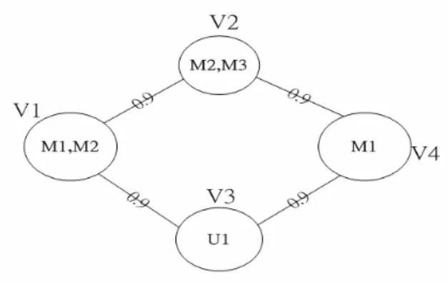
= i n k i i i i i i n i i i i i i i i i i t t where t S R t S R t S R t S R t S R t S R t S R t t S RHere we give an example as shown in Figure 5:
In the following examples, we have four nodes:
If the physical link reliability is 0.9 ,and the present traffic load is at a high busy rate of 95%,we can then use linear regression to get a lower probability that the link can work well as follows. If TR(ei)=0.9
Figure 5: Mobility patterns
3.6: Moving patterns
Moving patterns record users' behaviors. This is achieved by using a method to mine the moving patterns from the previous data log. With the moving patterns, we can develop a data allocation scheme for proper allocation of personal and shared data.
Table 2: Moving frequency matrix count V1 V2 v3 v4 V1v2 200 0 0 300 V1v3 250 0 0 250 V2v1 0 300 200 0 V2v4 0 100 400 0 V3v1 0 150 350 0 V3v4 0 450 50 0 V4v2 250 0 0 250 v4v3 350 0 0 150
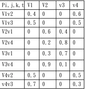
Table 3: Transition Probability Matrix Pi,j,k,t V1 V2 v3 v4 V1v2 0.4 0 0 0.6 V1v3 0.5 0 0 0.5 V2v1 0 0.6 0.4 0 V2v4 0 0.2 0.8 0 V3v1 0 0.3 0.7 0 V3v4 0 0.9 0.1 0 V4v2 0.5 0 0 0.5 v4v3 0.7 0 0 0.3
Since we take into account the probability that user may move from his current node to neighbor nodes, we must use the summation of the product of the static remote media access probability of the neighbor node and its transition probability to represent the remote media access probability for the mobile environment.
))
(
)
((
RMAP(U)
j jP
ijkt×
RMAP
N
=
∑
Suppose the following:
Assume user 1 came from E, and is now at F now. He needs media M1, M2, and M3 for his learning mission.
Figure 6: RMAP pattern
We need to compute the remote media access probability RMAP(F). And suppose that the transition probability from EF to neighbors B,E,G,J are 0.2,0.3,0.3,0.2 respectively. Then RMAP(F) is formulated as follows.
3.7: Data allocation
Distributed multimedia applications have played an important role in the recent advances in mobile learning environments. In such environments, storage volume can be quite large and as a result, we need to find a way to allocate courseware unit to improve the learning efficiency. Data allocation improves access reliability to the courseware unit. The purpose of this is to find a way to allocate the course material appropriately in a real network environment. From this, we can provide a higher standard of service to subscribers. The Data allocation strategy is as follows:
Our purpose is to find a way to allocate the course material into the real network environment.
We propose using the 「 Bread First Search 」 algorithm to traverse the graph below and transform it into a tree structure. The starting point is the user’s position.
Figure 7: DMDB network
The figure below is the result after transforming the graph from the previous page into a tree structure.
We then classify the media, and sequentially allocate the media into the physical network according to the defined order.
Figure 8: Tree structure of media
These are the basic steps used to determine potential paths through nodes. In the physical view we used link probability to model the network, multi-access to model the access probability, and moving patterns to improve the data allocation scheme.
Chapter 4
Logical View
In chapter 3, we discussed, from a physical view perspective, how we model link probability and how we strategize data allocation. We also used moving patterns to improve the data allocation scheme.
In this chapter, we introduce the concept of the Logical View and how we apply the branching algorithm to solve course planning problems. The Logical view discusses the course planning strategy to find a suitable way for learners to learn a particular course.
In addition, we discuss the methodology of helping students create their own study timetables to complete a curriculum based on the experiences of educationists. For this, we will introduce how we use the course planning strategy (section 4.4) to allocate the courseware units into the physical network (section 4.5) and run the simulations. And talk about the quiz problem and time restriction problem in section 4.8 and section 4.9, respectively.
4.1 The Learning sequence Environments
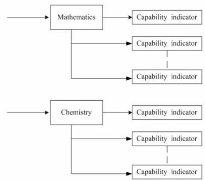
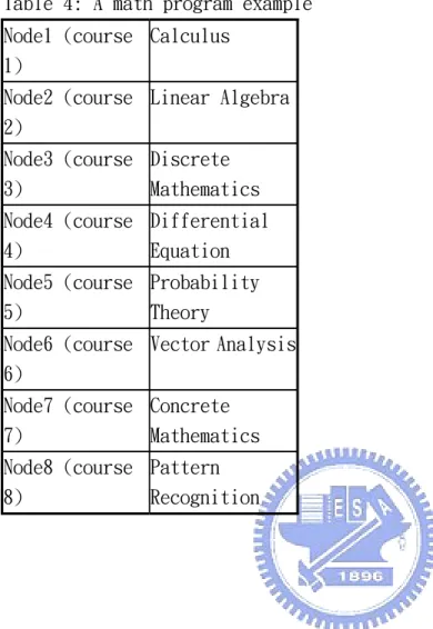
Learning sequence environments introduces the concept of the learning environment and the concept of mapping real e-learning courseware unit to the physical network topology, in other words from the logical view to the physical view. The reason for this is that, by doing so a network environment will provide better performance for learners to access course material. For example, Table 4 shows the entire contents of a math syllabus (calculus, linear algebra, discrete mathematics and so on). Each courseware unit has a capability indicator. Briefly, a capability indicator is used to describe a particular measurement (or capability factor a course provides) to the learner studying that a particular courseware unit and forms the basis for determining the capability for a learner to study another courseware unit. Each courseware unit can have several capability indicators (depicted in Figure 9).
Figure 9: The Capability Indicator structure
Capability indicators are useful because they assist us with the management of the courseware unit, for example, the distribution of difficulty of each courseware unit and so on. Thus, in order to complete a curriculum, a learner has to obtain a certain number of capability indicators. We thus use capability indicators in our proposed model and apply it to the directed graph. When the courseware unit capability indicator has been transferred into a directed graph, we apply the minimum weight branching algorithm to find the learning sequence based on the imposed requirements. The purpose of minimum weight branching (which will be discussed further in section 4.4) is to find an efficient learning path from a directed graph. The outcome of the learning sequence once minimum weight branching has been applied is mapped to the physical network environment using the data allocation scheme (discussed previously, in chapter 3).
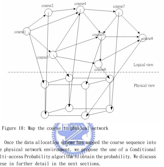
Figure 10 shows that the idea of mapping logical courseware unit into a physical network environment. The nodes in the logical view are logical capability indicator relations.
Table 4: A math program example Node1 (course 1) Calculus Node2 (course 2) Linear Algebra Node3 (course 3) Discrete Mathematics Node4 (course 4) Differential Equation Node5 (course 5) Probability Theory Node6 (course 6) Vector Analysis Node7 (course 7) Concrete Mathematics Node8 (course 8) Pattern Recognition
Figure 10: Map the course to physical network
Once the data allocation scheme has mapped the course sequence into the physical network environment, we propose the use of a Conditional Multi-access Probability algorithm to obtain the probability. We discuss these in further detail in the next sections.
4.2 Notations
Course n: It means the courseware unit n in the logical view Site n: It means the location n that holds courseware unit in the
physical view
CMP: Conditional Multi-access Probability
4.3 Assumptions and goals of course planning
In the previous section, we briefly introduced an overview to the concept of courseware unit relations, the application of minimum weight branching, dispatching them into the physical network environment, and using conditional Multi-access Probability to obtain the probability.
learning path (i.e. a sequence of courseware unit).
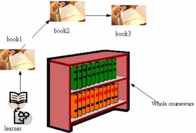
Figure 11: Idea of learning path
Suppose we have a book shelf (depicted in Figure 11) in the subject of mathematics. The bookshop can be depicted as an entire courseware unit selection in the curriculum. Each courseware unit (for example, algebra, geometry, discrete mathematics, vector analysis and so on) contains one or more capability indicators. The idea of learning paths is to find some books (courseware unit) that need to be studied in order to obtain all the capability indicators that are required. In the example depicted in figure 11, the learner needs to study book 1, book 2 and book 3 in order to obtain the required capability indicators and complete his curriculum. The purpose of this learning path is to save the learner's time by advising a proposed course plan.
In the next section we introduce the minimum weight branching algorithm and discuss how it is applied to the directed graph to produce a learning sequence path.
4.4. Minimum Weight Branching
4.1.1 Minimum Branching Overview
In the previous section we discussed our goal of finding an efficient learning path. This is achieved through the application of the minimum
weight branching algorithm. In an e-learning environment, we can apply Minimum Weight Branching to find the least difficult learning path.
Minimum weight branching [27] works in the following way:
A natural analog of a spanning tree in a directed graph is branching (also called arborescence). For a directed graph G and a vertex r, a branching rooted at r is an acyclic sub graph of G in which each vertex but r has exactly one outgoing edge, and there is a directed path from any vertex to r. This is also sometimes called an in-branching. By replacing “outgoing" in the above definition of a branching to “incoming," we get out-branching. An optimal branching of an edge-weighted graph is the branching of minimum total weight. Unlike the minimum spanning tree problem, optimal branching cannot be computed using a greedy algorithm. Edmonds gave a polynomial time algorithm to find optimal branching.
Suppose the following: let G=(v ,e) be an arbitrary graph, let r be the root of G, and let w(e) be the weight of edge e. Consider the problem of computing an optimal branching rooted at r. In the following discussion, assume that all edges of the graph have a nonnegative weight. In the first, we will give a directed graph, weight of every edge, the position of root node. The goal is to find a tree structure that is minimum weight of total edge weight.
4.4.2 Example
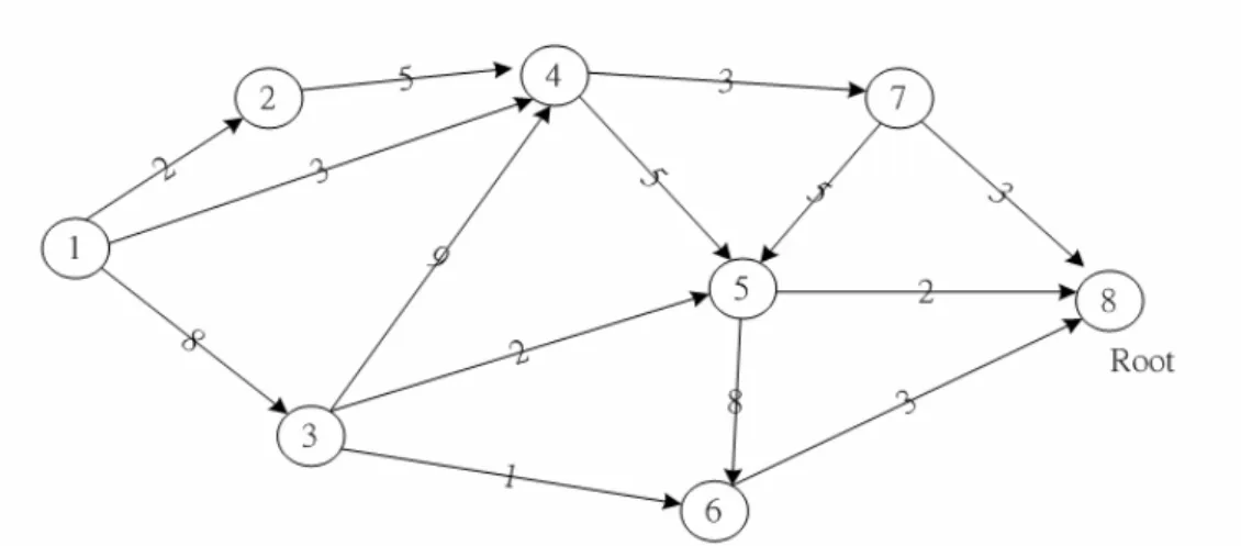
Suppose we would like to find the least difficult path for a learner to completing a curriculum. In this example, we use eight nodes (courses). The root is at node eight and we would like to find the learning sequence path using minimum weight branching. Figure 12 shows the relationships between courseware units. Each node represents one course. The direction of arrows depicts the order of relations with respect to one another. Each arrow is depicted by a difficulty level. In this example, our goal is to find learning sequence path for each node to node eight. Suppose a learner is currently at node 1, he has the choice of choosing either node 2, node 3 or node 4 as possible next stage courses. This process continues until the learner reaches node 8 and all possible paths to node 8 are exhausted. In total, there are 8 possible paths with varying difficulties to completing the curriculum. To find the best sequence (i.e. the path with the least difficulty); we apply the minimum weight branching algorithm.
Figure 12: Relationship of courseware unit
Figure 12 depicts the initial relationships between each courseware unit. After applying the minimum weight branching algorithm to find the best learning path, we obtain our result, depicted in Figure 13.
Figure 13: Branching of the relations
As a result, the best learning path for the learner at node 1 is node 1 -> node 4 -> node 7 -> node 8, and the difficulty is 9 (3+3+3)
Here we state all the learning paths and their difficulties.
z Learning path from node 1 is to take another 3 courses (in node 4, 7, 8), and the difficulty is 9(3+3+3).
z Learning path from node 2 is to take another 3 courses (in node 4, 7, 8), and the difficulty is 11(5+3+3).
z Learning path from node 3 is to take another 2 courses (in node 6, 8), and the difficulty is 4(1+3).
z Learning path from node 4 is to take another 2 courses (in node 7, 8), and the difficulty is 6(3+3).
z Learning path from node 5 is to take another 1 course (in node 8), and the difficulty is 2
z Learning path from node 6 is to take another 1 course (in node 8), and the difficulty is 3
z Learning path from node 7 is to take another 1 course (in node 8), and the difficulty is 3.
Depending on where a learner is in the physical network, the minimum weight branching algorithm can be used effectively to find the best learning path to node 8.
In the next section, we discuss the process of using data allocation to allocate the courseware unit in the physical network environment (i.e. the process of mapping the logical view to the physical view). We also discuss the use of a conditional Multi-access Probability algorithm to compute the resultant probability.
4.5 Using data allocation to allocate courseware unit in the
physical network and compute the probability
In the previous section we discussed using minimum weight branching to find the learning paths in a graph. In this section, we propose using a data allocation scheme to put the courseware unit in a physical setting, such as the physical network environment in a defined order. As we mentioned previously in section 4.2, under the capability indicator structure, each courseware unit is related to other units. Thus, after using the minimum weight branching algorithm to determine the learning sequence, we then use data allocation to assign the courseware unit into the physical network environment (discussed previously in chapter 3). Having done this, we then apply a conditional multi-access probability algorithm to obtain the resultant probability.
4.5.1 Conditional Multi-access Probability
The proposed conditional Multi-access Probability algorithm is a modified version based on the original Multi-access Probability algorithm (discussed in chapter 3). We use the modified algorithm because courseware unit is defined in a specific order.
After a request is sent by a user, the material provider may need to send several resources back. The access time of these resources may not be equal. The following is the definition of multi-access in ordered sequence reliability for courseware unit Si:
) | | Pr( P ) .... | ( .... ) | ( ) | ( ) Pr( max i 1 1 2 1 3 1 2 1 t t S where P P P P P P P P P user i i n n i = × × × × = − 4.5.2 Assumptions
We use Conditional Multi-access Probability to model the problem. Initially, given the course relations (capability indicator obtained), difficulties, reliability of each link and physical network topology, our goal is to allocate these courses in a specific order that decreases difficulty and increases access reliability.
4.5.3 Example
In this example, we explain the entire process of finding the learning sequence (using the minimum weight branching algorithm), allocating them into the physical network (using the data allocation scheme) and computing the probability (using the conditional Multi-access Probability algorithm).
Suppose we are given the following courseware unit relations and the physical network topology as shown in Figure 14. Suppose the user is at site 5 and begins with course 3. Assume each link probability (in the physical network topology) is 0.9. We would like to find the best learning path for the learner.
Figure 14 course relation and physical network topology
We summarize this process below:
z Step 1.: Apply the minimum weight branching algorithm to generate the learning path (depicted in Figure 15)
z Step 2: Find learning path for learner (in this example the learning path is course 3 -> course 6 -> course 8).
z Step 3: Allocate course of learner into physical network using the data allocation scheme
z Step 4: compute the CMP.(conditional Multi-access Probability) to find the resultant probability
Figure 16: Data allocation tree for mesh physical network
After applying the data allocation scheme (step 3), we find the result that:
z course 3 is in site 5
z course 6 is in site 4, and z course 8 is in site 2
This is depicted in Figure 16 and Figure 17.
Figure 17:A simple Mesh connected network
Using CMP (Conditional Multi-access Probability) to compute the probability, we get the following answer:
CMP (User) =Pr (course2)*Pr (course4| course 2)*Pr (course 8| course 2, course 4) = 0.5904899878335
In this sub-section we run some simulations to present the results for all the possible probabilities supposing the learner is at different sites. From Figure 16, simulation 1 supposes the learner is at site 1, simulation 2 supposes the learner is at site 2...and so on.
Simulation 1: CMP (User) =Pr (2)*Pr (4|2)*Pr (6|2, 4) =0.9304899878335 Simulation 2: CMP (User) =Pr (2)*Pr (4|2)*Pr (8|2, 4) =0.9304899878335 Simulation 3: CMP (User) =Pr (2)*Pr (6|2) =0.8095491254 Simulation 4: CMP (User) =Pr (2)*Pr (6|2) =0.8095491254 Simulation 5: CMP (User) =Pr (8) =0.899395994 Simulation 6: CMP (User) =Pr (8) =0.899395994 Simulation 7: CMP (User) =Pr (8) =0.899395994
In Figure 18 and Figure 19 we graph the simulation results. In Figure 18, the x-axis represents the number of courses taken by a learner and the y-axis represents the successful probability. In Figure 19, the x-axis represents the number of courses taken by a learner and the y-axis the difficulty of the courses.
Figure 18: Successful probability
In Figure 18, we note that as the number of courses increase, the probability decreases meaning there is a low probability of success when learning several courses. In Figure 19, we note that as the number of courses a learner studies increases, the difficulty increases.
In the next two sections (section 4.6 and section 4.7), we present the quiz paper problem and the time restriction problem as two examples that effectively demonstrate the applicability of our approach.
4.6 The Quiz Paper problem
The Quiz paper problem is based on achieving a particular goal of a learner based on statistics from past history quiz papers. The idea of this problem is that learners can know what they need to learn based on past quiz statistics. For example, Figure 20 depicts a database of examination papers. This database contains several questions from past examination papers. Each of these questions has a capability indicator and distribution. The distribution refers to the frequency of that particular question in the database that has been used for quiz or test (e.g. question 1 has a capability indicator of 9-a-01 and distribution of 14.5%, question 2 has a capability indicator 9-a-02 and a distribution of 28.6% and so on).
Figure 20: Data Base of examination
In section 4.6.1 we state our assumptions and in section 4.6.2 will present an example.
4.6.1 Assumptions
The goal of this example is for a learner to achieve a predefined score.
4.6.2 Example
Suppose a student needs to achieve 60% of the grade in the Quiz paper, and the only information about the examination is the history of quiz paper statistics. In this example, suppose we have 4 nodes (questions with capability indicators), and assume the following capability indicators and distributions for the following questions:
z Question 1 with a capability index of 9-a-02 and distribution of 28.6% z Question 2 with a capability index of 9-a-03 and distribution of 14.5% z Question 3 with a capability index of 9-a-05 and distribution of 28.6% z Question 4 with a capability index of 9-a-08 and distribution of 28.6%
Figure 21 shows the distribution of past statistics and present them in the directed graph.
Figure 21: course distribution We then undertake the following steps:
z We Input a grade to be achieved, e.g. 60% of the grade in the Quiz paper.
z We have the distributions for these questions according to the past history of examinations as well as the capability indicators
Figure 22: Results of the quiz paper
To determine the learning path, we consider two factors. First, the difficulty levels associated with each question and the distribution of each question. The difficulty levels associated with each particular question takes precedence over the distribution percentage of the question in determining the learning path.
Figure 22 demonstrates the step-by-step process to the discovery of the learning path. In step 1, we obtain a distribution of 28.6%, and then we use the difficulty level to determine which questions (question 2 or question 3) to study next. The difficulty to question 2 is lower than that of question 3, so in step 2, we study question 2 (which has a distribution of 14.5%). In step 3, the difficulty to question 4 is higher than the difficulty to question 3, so we study question 3 (which has a distribution of 28.6%). At this point we have achieved 60% (in fact we have achieved 71.7%), thus achieving our goal set out earlier.
4.7 The Time restricted problem
The Time Restricted Problem deals with some learners who have time constraints for some reasons. In this example, our goal is to meet their requirements within this time constraint. We map the TLCS (Time Limited Candidate Selector) algorithm [28] to distribute time over the learning path. We find time constraints particularly important because time factors can play an important role in exam preparation.
4.7.1 Assumptions
We share the given time (requested by the learner) to the required courses (after we have applied the minimum weight branching algorithm to find his learning sequence). Two important parameters in this problem
are “learning curves" and “pre-requests" (which we discuss further in section 4.7.2 and section 4.7.4 respectively). In the Time Restricted Problem, we are given the following parameters:
z the time constraints z the difficulty levels z the learning curve and z the course relations
4.7.2 Learning curves
The concept of learning curve is that when learning a course, if we spend more time, the score should be higher, we use figure 23 to show this concept. The X-axis is time and the y-axis is performance the learner achieves. 100% is the highest possible score.
Figure 23: Learning curve
4.7.3 Example
Suppose we have eight courses (Table 5) depicted in the directed graph shown in Figure 24. Each course has an examination date. The examination dates for each course are listed in the table. We assume that the learning curve of each course is one month (meaning that the learner must spend one or more months studying the course in order to pass). The learner starts with calculus (course1), and the given time constraint is the examination due date. Our goal is to reach (pass exams) course 8 given the time constraints distributed across the learning path and the starting time is in January 1.
Table 5: The courseware unit Course1 Calculus(exam in April)
Course2 Linear Algebra(exam in March)
Course3 Discrete Mathematics(exam in April) Course4 Differential Equation(exam in June) Course5 Probability Theory(Exam in June) Course6 Vector Analysis(exam in July) Course7 Concrete Mathematics(exam in July) Course8 Pattern Recognition(exam in November)
Figure 24: Relations of the courseware unit
First, we apply the Minimum weight branching algorithm to the directed graph (in Figure 24) to get learning path in Figure 25。
Our result is four learning paths:
z path 1:Course1ÆCourse4ÆCourse7ÆCourse8 z Path 2:Course2ÆCourse4ÆCourse7ÆCourse8 z Path 3:Course3ÆCourse6ÆCourse8
z Path 4:Course5ÆCourse8
Because the learner begins at course 1 (calculus), his learning path is path 1(Course1ÆCourse4ÆCourse7ÆCourse8). We map the TLCS algorithm to sequence the four courses.
1. Sequence the courses in list E.
2. If no courses in list E are late, stop, otherwise, identify the first late course, k.
3. Identify the latest position in the list in which the course k would not be late. Place course k in that position if it does not make any of the courses before k late, otherwise place it in late List L. Revise the sequence in list E and return to step 2.
According to TLCS algorithm, in step 1, the sequence in E is path 1(course1->course4->course7->course8). In step 2, we check if there is any late course (e.g. course 1 exam is in April and we need 1 month to study, therefore the time is enough). There in no course that is late. At this point, we distribute our time constraint to these four courses. First we distribute the whole of January to course 1 (we assume the learning curve requires one month at least) and test in April. We then share 1 month (whole of February) to course 4 and test in June, and then share 1 month (whole of March) to course 7 and test in July, and finally, share 1 month (whole of April) to course 8 and test in November. Under this arrangement, the learner can prepare his course sufficiently before tests.
4.7.4 Pre-requests
In time restriction problem, we discussed time sharing problem. However, in some cases, we might encounter “pre-request" courses. The concept of a “pre-request" course states that when a learner completes a particular course, the learning curve will change. Courses that apply
this concept are called “pre-request" courses.
Figure 26 shows four learning curves, we note that after completing a pre-request course, the learning curve changes from learning curve 1 to learning curve 2 and so on.
Figure 26: Score percentage
Example
Suppose the learning curve is typically 2 months for each course and the pre-request course is course 3. After finishing course 3, learning curve for each course becomes 1 month under the “pre-request" concept.
Suppose the learner begins at course 1 and the time constraint is 7 months. The directed graph for this is depicted in Figure 27. We approach this problem using two methods.
Method 1:
In this method, under normal conditions, we attempt to find the learning path.
First, we use the minimum weight branching algorithm to obtain the learning path in figure 28.
Figure 28
The learning paths are as follow:
path 1: Course1ÆCourse4ÆCourse7ÆCourse8 Path 2: Course2ÆCourse4ÆCourse7ÆCourse8 Path 3: Course3ÆCourse6ÆCourse8
Path 4: Course5ÆCourse8
Since the learner starts from course 1, we use path 1 and distribute the 7 months to these courses (Course1ÆCourse4ÆCourse7ÆCourse8), noting that we need a minimum of 2 months per course:
z course 1:2 months z course 4:2 months z course 7:2 months z course 8: 2 months
We note that the total is 8 months, thus, over our time constraint limitation of 7 months. We find that, under normal conditions, this method does not achieve our goal.
In the next method, we attempt to find the learning path in the directed graph that contains “pre-request" courses.
Method 2:
We suppose that course 3 is a pre-request course. If the learner starts from course one, the next logical course will be the pre-request course (i.e. course 3). From there on, we continue to follow the learning path in Figure 28 to course 8. Thus, our path is (course 1 -> course 3 -> course 6 -> course 8). We show the time distribution below:
z course 1: 2 months z course 3: 2 months
z course 6:1 month (it becomes one our because of pre-request course 3)
z course 8: 1 month
In this method, our total months spent is 6 months – achieving our goal within the time constraint of 7 months.
The results are shown below in figure 29.
Figure 29: Result learning path
Having demonstrated the above two-methods, we can conclude that if a directed graph contains a pre-request course, method one is not suitable, in other words, using our original algorithm. So, we modify our algorithm in method 2 (by changing the learning path to suit the pre-request course)
to suit the pre-request course.
Summary
In this chapter, we discussed our model and how it maps the logical view to the physical view. First, we obtained a directed graph containing difficulty levels, time constraints, capability indicators, course relations and later, learning curves. Using the minimum weight branching algorithm, we were able to find the learning path of the user that took these parameters into account and modeled them in the physical environment. We demonstrated the applicability of this approach through several examples.
In chapter 5 we will demonstrate the applicability of our model into some physical networks such as the ARPA network, the pacific basin network and so forth.
Chapter 5
Illustrative examples and simulation results
In this chapter, we use some examples to see the course access reliability from the logical to the physical view. We demonstrate the applicability of this in four different physical networks: The ARPA network, The Pacific Basin Network, the TANet network and the three-Cube Network. In this chapter, we use the logical view that depicted in the figure 24 as an example and applied it into the physical network mentioned above. Figure 25 is redrawn as Figure 30, and map the courseware unit into the physical network, compute the difficulties of each learning path and their successful probability in the physical network.
Figure 30: Learning paths
All the possible Paths for each course in Figure 30: Path for course 1: Course1ÆCourse4ÆCourse7ÆCourse8 Path for course 2: Course2ÆCourse4ÆCourse7ÆCourse8 Path for course 3: Course3ÆCourse6ÆCourse8
Path for course 4: Course7ÆCourse8 Path for course 5: Course5ÆCourse8 Path for course 6: Course6ÆCourse8 Path for course 7: Course7ÆCourse8
Consider the physical network topology in figure 31 which consists of 21 nodes, the user is in node 11; there are 26 links, and other data storage locations.
Figure 31: ARPA network
The Allocation tree of ARPA network is depicted below:
Figure 32: Allocation of ARPA network
We wish to determine the probability that a user can finish a course successfully in the ARPA network environment.
simulation 1 starts at course one, simulation 2 starts at course two and so on. Our results are as follows:
Simulation 1
z Simulation 1 needs to take another 3 courses (c4, c7 and c8 in figure 32 and Figure 30)
z the difficulty is 9(3+3+3)
z Its allocation site is 9, 12,14,7 in APRA network (figure 31). Simulation 2
z Simulation 2 needs to take another 3 courses (c4,c7,c8 in figure 32 and Figure 30)
z the difficulty is 11(5+3+3),
z Its allocation site is site 9, 12,14,7 in APRA network (figure 31). Simulation 3
z Simulation 3 needs to take another 2 courses (c 6,c8 in figure 32 and Figure 30)
z and the difficulty is 4(1+3),
z Its allocation site is site 9, 12, 14 in APRA network (figure 31). Simulation 4
z simulation 4 needs to take another 2 course(c 7,c8 in figure 32 and Figure 30)
z and the difficulty is 6(3+3),
z Its allocation site is site 9, 12, 14. (Figure 31). Simulation 5
z Simulation 5 : it need to take another 1 course(c 8, in figure 32 and Figure 30)
z and the difficulty is 2,
z Its allocation site is site 9, 12 in APRA network (figure 31). Simulation 6
z simulation 6 needs to take another 1 course(c 8, in figure 32 and Figure 30)
z and the difficulty is 3,
z Its allocation site is site 9, 12(figure 31). Simulation 7
z simulation 7 : it need to take another 1 course(c 8, in figure 32 and Figure 30)
z and the difficulty is 3,
z Its allocation site is site 9, 12 in APRA network (figure 31). Table 6 shows the results (Success ratio) of applying conditional Multi-access Probability to the physical APRA network from course 1 to course 8.
Table 6: Simulation result of APRA network
Course C1 C2 C3 C4 Success ratio 0.95 0.9301 0.9116684 0.8967487 Course C5 C6 C7 C8 Success ratio 0.88456843 0.8164889 0.756879874 0.7148863
Pacific Basin network:
Consider the network topology in figure 33 which consists of 19 nodes, the user is in node 7; there are 26 links, and other data storage locations.
I
Figure 33: Pacific Basin network
In this example, we need to allocate 8 media. The total access reliability uses conditional Multi-access Probability. The tree of the physical network is displayed below in Figure 34
We wish to determine the probability that a user can finish a course successfully in the Pacific Basin network environment.
From figure 34, suppose we run simulations from all courses, for example, simulation 1 starts at course one, simulation 2 starts at course two and so on. Our results are as follows:
Simulation 1
z Simulation 1 needs to take another 3 courses (c4, c7 and c8 in figure 34 and Figure 30)
z the difficulty is 9(3+3+3)
z Its allocation site is 6,8,9,3 in the physical network (figure 34). Simulation 2
z Simulation 2 needs to take another 3 courses (c4,c7,c8 in figure 34 and Figure 30)
z the difficulty is 11(5+3+3),
z Its allocation site is site 6,8,9,3 in the physical network (figure 34).
Simulation 3
z Simulation 3 needs to take another 2 courses (c 6,c8 in figure 34 and Figure 30)
z and the difficulty is 4(1+3),
z Its allocation site is site 6, 8, 9 in the physical network (figure 34).
Simulation 4
z simulation 4 needs to take another 2 course(c 7,c8 in figure 34 and Figure 30)
z and the difficulty is 6(3+3),
z Its allocation site is site 6, 8, 9. (Figure 34). Simulation 5
z Simulation 5 : it need to take another 1 course(c 8, in figure 34 and Figure 30)
z and the difficulty is 2,
z Its allocation site is site 6, 8 in the physical network (figure 34). Simulation 6
z simulation 6 needs to take another 1 course(c 8, in figure 34 and Figure 30)
z and the difficulty is 3,
z Its allocation site is site 6, 8(figure 34). Simulation 7
z simulation 7 : it need to take another 1 course(c 8, in figure 34 and Figure 30)
z and the difficulty is 3,
z Its allocation site is site 6, 8 in the physical network (figure 34). Table 7 shows the results (Success ratio) of applying conditional Multi-access Probability to the physical Pacific Basin network from course 1 to course 8.
Table 7: simulation result of Pacific Basin network
Course C1 C2 C3 C4 Success ratio 0.90 0.83474767 0.801546323 0.79654851 Course C5 C6 C7 C8 Success ratio 0.754684132 0.73546454 0.731544842 0.71488512 TANet topology:
Consider the physical network topology in figure 35 which consists of 9 nodes, the user is in node 4; there are 14 links, and other data storage locations.
Figure 35: TANet topology
Figure 36: Allocation of TANet
We wish to determine the probability that a user can finish a course successfully in the TANet network environment.
From figure 36, suppose we run simulations from all courses, for example, simulation 1 starts at course one, simulation 2 starts at course two and so on. Our results are as follows:
Simulation 1
z Simulation 1 needs to take another 3 courses (c4, c7 and c8 in figure 36 and Figure 30)
z the difficulty is 9(3+3+3)
z Its allocation site is 2,1,5,6 in the physical network (figure 36). Simulation 2
z Simulation 2 needs to take another 3 courses (c4,c7,c8 in figure 36 and Figure 30)
z the difficulty is 11(5+3+3),
z Its allocation site is site 2,1,5,6 in the physical network (figure 36).
Simulation 3
z Simulation 3 needs to take another 2 courses (c 6,c8 in figure 36 and Figure 30)
z
z and the difficulty is 4(1+3),
z Its allocation site is site 2, 1, 5 in the physical network (figure 36).
Simulation 4
z simulation 4 needs to take another 2 course(c 7,c8 in figure 36 and Figure 30)
z and the difficulty is 6(3+3),
z Its allocation site is site 2, 1, 5. (Figure 36). Simulation 5
z Simulation 5 : it need to take another 1 course(c 8, in figure 36 and Figure 30)
z and the difficulty is 2,
z Its allocation site is site 2, 1 in the physical network (figure 36). Simulation 6
z simulation 6 needs to take another 1 course(c 8, in figure 36 and Figure 30)
z and the difficulty is 3,
Simulation 7
z simulation 7 : it need to take another 1 course(c 8, in figure 36 and Figure 30)
z and the difficulty is 3,
z Its allocation site is site 2, 1 in the physical network (figure 36). Table 8 shows the results (Success ratio) of applying conditional Multi-access Probability to the physical TANet network from course 1 to course 8.
Table 8: Simulation of TANet
Course C1 C2 C3 C4 Success ratio 0.90 0.85456346 0.822345432 0.79345435 Course C5 C6 C7 C8 Success ratio 0.78604895 0.73104895 0.729867474 0.71204576 3-Cube network:
Consider the physical network topology in figure 37 which consists of 8 nodes, the user is in node 1; there are 12 links, and other data storage locations.