以函數鏈結為基礎之類神經模糊網路及其應用

(1)

國

立

交

通

大

學

電機與控制工程學系

博

士

論

文

以函數鏈結為基礎之類神經模糊網路及其應用

A Functional-Link-Based Neuro-Fuzzy Network and Its Applications

研

研究

究

究生

究

生

生：

：

：陳政宏

陳政宏

指導教授

指導教授：

：

：林進燈

林進燈

中

中華

華

華民

華

民

民國

國

國九

九

九十

九

十七

十

七

七年

七

年

年七

七

七月

月

(2)

以函數鏈結為基礎之類神經模糊網路及其應用

A Functional-Link-Based Neuro-Fuzzy Network and Its

Applications

研究生：陳政宏

Student：Cheng-Hung Chen

指導教授：林進燈博士

Advisor：Dr. Chin-Teng Lin

國立交通大學

電機與控制工程學系

博士論文

A Dissertation

Submitted to Department of Electrical and Control Engineering

College of Electrical Engineering

National Chiao Tung University

in partial Fulfillment of the Requirements

for the Degree of

Doctor of Philosophy

in

Electrical and Control Engineering

July 2008

Hsinchu, Taiwan, Republic of China

(3)

國

立

交

通

大

學

國

立

交

通

大

學

國

立

交

通

大

學

國

立

交

通

大

學

博碩士論文全文電子檔著作權授權書

(提供授權人裝訂於紙本論文書名頁之次頁用)

本授權書所授權之學位論文，為本人於國立交通大學電機與控制工程系所

＿＿＿＿＿＿組，九十六學年度第二學期取得博士學位之論文。

論文題目：以函數鏈結為基礎之類神經模糊網路及其應用

指導教授：林進燈

■ 同意 □不同意

本人茲將本著作，以非專屬、無償授權國立交通大學與台灣聯合大學系統圖

書館：基於推動讀者間「資源共享、互惠合作」之理念，與回饋社會與學術

研究之目的，國立交通大學及台灣聯合大學系統圖書館得不限地域、時間與

次數，以紙本、光碟或數位化等各種方法收錄、重製與利用；於著作權法合

理使用範圍內，讀者得進行線上檢索、閱覽、下載或列印。

論文全文上載網路公開之範圍及時間：

本校及台灣聯合大學系統區域網路 ■ 中華民國 99 年 2 月 23 日公開

校外網際網路

_{■ 中華民國 99 年 2 月 23 日公開}

授

權

人

人：

人

：

：陳政宏

陳政宏

親筆簽名

親筆簽名：

：

中華民

中華民國

國

97 年

年

7 月

月

30 日

日

(4)

國

立

交

通

大

學

國

立

交

通

大

學

國

立

交

通

大

學

國

立

交

通

大

學

博碩士紙本論文著作權授權書

(提供授權人裝訂於全文電子檔授權書之次頁用)

本授權書所授權之學位論文，為本人於國立交通大學電機與控制工程系所

＿＿＿＿＿＿組，九十六學年度第二學期取得博士學位之論文。

論文題目：以函數鏈結為基礎之類神經模糊網路及其應用

指導教授：林進燈

■ 同意

本人茲將本著作，以非專屬、無償授權國立交通大學，基於推動讀者間「資

源共享、互惠合作」之理念，與回饋社會與學術研究之目的，國立交通大學

圖書館得以紙本收錄、重製與利用；於著作權法合理使用範圍內，讀者得進

行閱覽或列印。

本論文為本人向經濟部智慧局申請專利(未申請者本條款請不予理會)的附

件之一，申請文號為：________________，請將論文延至年

月____日再公開。

授

權

人

人：

人

：

：陳政宏

陳政宏

親筆簽名

親筆簽名：

：

中華民

中華民國

國

97 年

年

7 月

月

30 日

日

(5)

國家圖書館

國家圖書館博碩士論文電子檔案上網授權書

博碩士論文電子檔案上網授權書

ID:GT009312816

本授權書所授權之論文為授權人在國立交通大學電機學院電機與控制工程系所

_________ 組九十六學年度第二學期取得博士學位之論文。

論文題目：以函數鏈結為基礎之類神經模糊網路及其應用

指導教授：林進燈

茲同意將授權人擁有著作權之上列論文全文（含摘要），非專屬、無償授權國

家圖書館，不限地域、時間與次數，以微縮、光碟或其他各種數位化方式將上

列論文重製，並得將數位化之上列論文及論文電子檔以上載網路方式，提供讀

者基於個人非營利性質之線上檢索、閱覽、下載或列印。

※ 讀者基於非營利性質之線上檢索、閱覽、下載或列印上列論文，應依著作權法相關規定辦理。

授權人

授權人：

：

：陳政宏

陳政宏

親筆簽名

親筆簽名：

：

中華民

中華民國

國

97 年

年

7 月

月

30 日

日

1. 本授權書請以黑筆撰寫，並列印二份，其中一份影印裝訂於附錄三之二(博碩士紙本論文著作權授權書)之次頁﹔另一份於辦理離校時繳交給系所助理，由圖書館彙總寄交國家圖書館。

(6)

中華民國 97 年 5 月

(7)

(8)

(9)

以函數鏈結為基礎之類神經模糊網路及其應用

研究生：陳政宏

指導教授：林進燈博士

國立交通大學電機與控制工程學系﹙研究所﹚博士班

摘要

本篇論文提出一以函數鏈結為基礎之類神經模糊網路及其相關學習演算法。此類神經模糊網路採用函數鏈結類神經網路當作模糊法則的後件部。此後件部是輸入變數的非線性組合，它是利用函數展開的方式，能在高維度的輸入空間中提供良好的非線性決策能力，因此，可使網路輸出更具體且更逼近目標輸出。本論文主要為三大部分。第一部份將詳細介紹以函數鏈結為基礎之類神經模糊網路及其線上學習演算法。此演算法包含架構學習及參數學習，架構學習是藉由熵的量測決定是否要增長一個新的法則，參數學習是使用倒傳遞演算法調整網路上的所有參數。由於倒傳遞演算法常常會得到局部最佳解。因此，在第二部份中，我們提出一改良式差分進化演算法，所提出的演算法與傳統差分進化演算法是不同的，在於我們使用一有效的搜尋機制使得每條個體能更新在目前最佳解和亂數搜尋解之間，並採用以群為基底的突變方式以提高個體間彼此的差異性。但以上的進化演算法，無法決定該使用多少法則數。因此，在第三部份中，我們提出一以法則為基礎的共生差分進化演算法。此演算法是利用多個子族群進行進化，每個子族群的個體代表每條模糊法則，且每個子族群能各自進化。此外，這演算法也能自動決定子族群數，並最佳化網路上的所有參數。最後，我們將與其他方法比較，以證實所提出的網路架構及其相關演算法之有效性。

(10)

A Functional-Link-Based Neuro-Fuzzy Network

and Its Applications

Student：Cheng-Hung Chen Advisor：Dr. Chin-Teng Lin

Department of Electrical and Control Engineering

National Chiao-Tung University

Abstract

This dissertation proposes a functional-link-based neuro-fuzzy network (FLNFN) and its related learning algorithms. The proposed FLNFN model uses a functional link neural network to the consequent part of the fuzzy rules. The consequent part uses a nonlinear functional expansion to form arbitrarily complex decision boundaries. Thus, the local properties of the consequent part in the FLNFN model enable a nonlinear combination of input variables to be approximated more effectively. This dissertation consists of three major parts. In the first part, the FLNFN model and an online learning are presented. The online learning algorithm consists of structure learning and parameter learning. The structure learning depends on the entropy measure to determine the number of fuzzy rules. The parameter learning, based on back-propagation, can adjust the shape of the membership function and the corresponding weights of the consequent part. Unfortunately, the back-propagation learning algorithm may reach the local minima very quickly. Therefore, a modified differential evolution (MODE) is presented to optimize the FLNFN parameters in the second part. The proposed MODE learning algorithm differs from the traditional differential evolution. The MODE adopts a method to effectively search between the best individual and randomly chosen individuals, and the MODE also provides a cluster-based mutation scheme, which maintains useful diversity in the population to increase the search

(11)

capability. But, the aforementioned algorithm cannot determine how many rules to be used. Therefore, a rule-based symbiotic modified differential evolution (RSMODE) is proposed for the FLNFN model in the third part. The RSMODE adopts a multi-subpopulation scheme that uses each individual represents a single fuzzy rule and each individual in each subpopulation evolves separately. Furthermore, the proposed RSMODE learning algorithm can also determine the number of rule-based subpopulation and adjust the FLNFN parameters. Finally, the proposed FLNFN model and its related learning algorithms are applied in various control problems. Results of this dissertation demonstrate the effectiveness of the proposed methods.

(12)

Acknowledgment

在這研究期間裡，首先要感謝我的博士班指導教授林進燈博士和碩士

班指導教授林正堅博士，在二位教授豐富的學識、殷勤的教導及嚴謹的督

促下，使我學習到許多的寶貴知識及在面對事情中應有的處理態度、方法，

並且在研究與投稿論文的過程中，二位教授有許多深入的見解及看法且對

於斟酌字句、思慮周延，更是我該學習的目標。師恩好蕩，指導提攜，銘

感於心。

由衷感謝口試委員傅立成教授、周至宏教授、洪宗貝教授、李祖聖教授、

蔡文祥教授及楊谷洋教授給予許多寶貴的建議與指正，使得這篇論文更加

完整。同時要感謝交大多媒體實驗室的學長劉得正博士及蒲鶴章博士還有

全體同學及學弟妹，在研究的過程中不斷的互相砥礪及討論。感謝過去

91 級朝陽資工系的所有同學，在這過程中，一起分享不同的經驗。感謝一路

走來陪伴身邊的所有朋友，使得我的研究生涯變得多采多姿。

特別要感謝我的父親、母親、妹妹，在這段日子中不斷的給予支持及鼓

勵，讓我能夠專心於研究的工作並完成博士學位。最後誠摯地以本論文研

究成果獻給我的師長、父母、家人及所有的朋友們。

陳政宏

九十七年七月二十七日

(13)

List of Tables

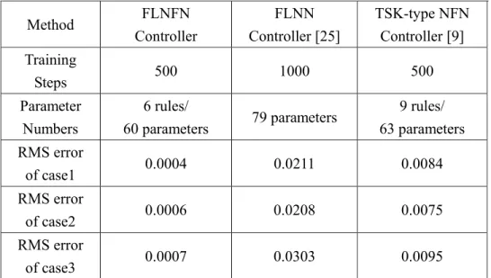
Table 2.1: Comparison of performance of various controllers to control of water bath temperature system...26 Table 2.2: Comparison of performance of various controllers to control of BIBO nonlinear

plant. ...31 Table 2.3: Comparison of performance of various controllers to control of ball and beam

system. ...33 Table 2.4: Comparison of performance of various controllers to control of MIMO plant...34 Table 3.1: Parameter settings before training. ...45 Table 3.2: Comparison of performance of various controllers to control of water bath

temperature system...49 Table 3.3: Comparison of performance of various controllers to control of the planetary train type inverted pendulum system with a 0.1s sampling rate. ...58 Table 3.4: Comparison of performance of various controllers to control of the magnetic

levitation system with a 0.1s sampling rate...69 Table 4.1: Parameter settings before training. ...81 Table 4.2: Comparison of performance of various controllers to control of water bath

temperature system...86 Table 4.3: Comparison of performance of various controllers to control of ball and beam

system. ...88 Table 4.4: Comparison of performance of various controllers to control of backing up the

(16)

List of Figures

Figure 2.1: Structure of FLNN. ...9

Figure 2.2: Structure of proposed FLNFN model. ... 11

Figure 2.3: Flow diagram of the structure/parameter learning for the FLNFN model...14

Figure 2.4: Conventional online training scheme...21

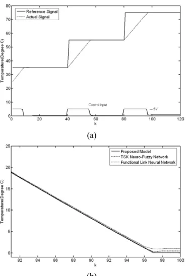
Figure 2.5: (a) Final regulation performance of FLNFN controller in water bath system. (b) Error curves of the FLNFN controller, TSK-type NFN controller and FLNN controller between k=81 and k=100. ...24

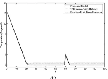
Figure 2.6: (a) Behavior of FLNFN controller under impulse noise in water bath system. (b) Error curves of FLNFN controller, TSK-type NFN controller and FLNN controller...25

Figure 2.7: (a) Behavior of FLNFN controller when a change occurs in the water bath system. (b) Error curves of FLNFN controller, TSK-type NFN controller and FLNN controller...25

Figure 2.8: (a) Tracking of FLNFN controller when a change occurs in the water bath system. (b) Error curves of FLNFN controller, TSK-type NFN controller and FLNN controller...26

Figure 2.9: Block diagram of FLNFN controller-based control system...27

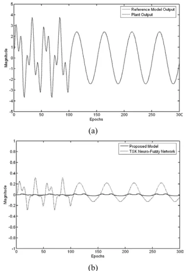
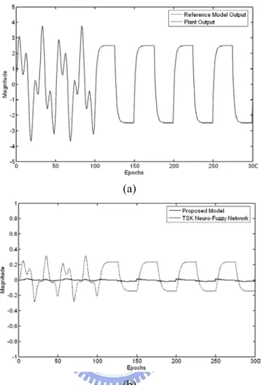
Figure 2.10: Final system response in first case of example 2. (a) The dashed line represents plant output and the solid line represents the reference model. (b) Error curves of FLNFN controller and TSK-type NFN controller...29

Figure 2.11: Final system response in second case of example2. (a) The dashed line represents plant output and the solid line represents the reference model. (b) Error curves of FLNFN controller and TSK-type NFN controller...29

Figure 2.12: Final system response in third case of example 2. (a) The dashed line represents plant output and the solid line represents the reference model. (b) Error curves of FLNFN controller and TSK-type NFN controller...30

Figure 2.13: Final system response in fourth case of example 2. The dashed line represents plant output and the solid line represents the reference model...30

Figure 2.14: Ball and beam system. ...31

Figure 2.15: Responses of ball and beam system controlled by FLNFN model (solid curves) and TSK-type NFN model (dotted curves) under four initial conditions...33

Figure 2.16: Responses of four states of ball and beam system under the control of the trained FLNFN controller. ...33 Figure 2.17: Desired output (solid line) and model output using FLNFN controller (dotted line)

of (a) Output 1. (b) Output 2 in Example 4. Error curves of FLNFN controller (solid line) and TSK-type NFN controller (dotted line) for (c) output 1 and (d)

(17)

output 2. ...35

Figure 3.1: An example of a two-dimensional cost function showing its contour lines and the process for generating vi,G+1. ...39

Figure 3.2: Illustration of the crossover process for N=7 parameters. ...40

Figure 3.3: Coding FLNFN into an individual in the proposed MODE method. ...41

Figure 3.4: A mutation operation in the modified differential evolution...44

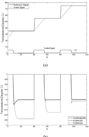
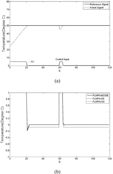
Figure 3.5: (a) Final regulation performance of FLNFN-MODE controller in water bath system. (b) Error curves of the FLNFN-MODE controller, FLNFN-DE controller and FLNFN-GA controller. ...46

Figure 3.6: (a) Behavior of FLNFN-MODE controller under impulse noise in water bath system. (b) Error curves of FLNFN-MODE controller, FLNFN-DE controller and FLNFN-GA controller...47

Figure 3.7: (a) Behavior of FLNFN-MODE controller when a change occurs in the water bath system. (b) Error curves of FLNFN-MODE controller, FLNFN-DE controller and FLNFN-GA controller...48

Figure 3.8: (a) Tracking of FLNFN-MODE controller when a change occurs in the water bath system. (b) Error curves of FLNFN-MODE controller, FLNFN-DE controller and FLNFN-GA controller...49

Figure 3.9: A physical model geometry of the planetary train type inverted pendulum. ...50

Figure 3.10: Control block diagram for the planetary train type inverted pendulum system. .53 Figure 3.11: The experimental planetary train type inverted pendulum system. ...54

Figure 3.12: (a)-(d) Final regulation performance of the FLNFN-MODE controller, PID controller, FLNFN-DE controller and FLNFN-GA controller. (e) Scaling curves of the FLNFN-MODE controller and PID controller between the 1.5th second and the 3.5th second. ...56

Figure 3.13: (a)-(d) Tracking of the FLNFN-MODE controller, PID controller, FLNFN-DE controller and FLNFN-GA controller, respectively, for a square wave with amplitude ±0.02 and frequency 0.5Hz. (e) Tracking curves of the FLNFN-MODE controller and PID controller between the 4th_{second and the 8}th second. ...58

Figure 3.14: Sphere and coil arrangement of the magnetic levitation system...59

Figure 3.15: Control block diagram for the magnetic levitation system. ...61

Figure 3.16: Experimental magnetic levitation system. ...62

Figure 3.17: (a)-(d) Experimental results of FLNFN-MODE controller, PID controller, FLNFN-DE controller and FLNFN-GA controller due to periodic sinusoidal command for reference position and actual position, tracking error and control effort. ...64 Figure 3.18: (a)-(d) Experimental results of FLNFN-MODE controller, PID controller,

(18)

FLNFN-DE controller and FLNFN-GA controller due to periodic square command for reference position and actual position, tracking error and control

effort. ...65

Figure 3.19: (a)-(d) Behavior of the FLNFN-MODE controller, PID controller, FLNFN-DE controller and FLNFN-GA controller under impulse noise in a magnetic levitation system for reference and actual positions, tracking error, and control effort. ...67

Figure 3.20: (a)-(d) Behavior of the FLNFN-MODE controller, PID controller, FLNFN-DE controller, and FLNFN-GA controller when a change occurs in the magnetic levitation system for reference and actual positions, tracking error, and control effort. ...69

Figure 4.1: Flowchart of the RSMODE learning algorithm...73

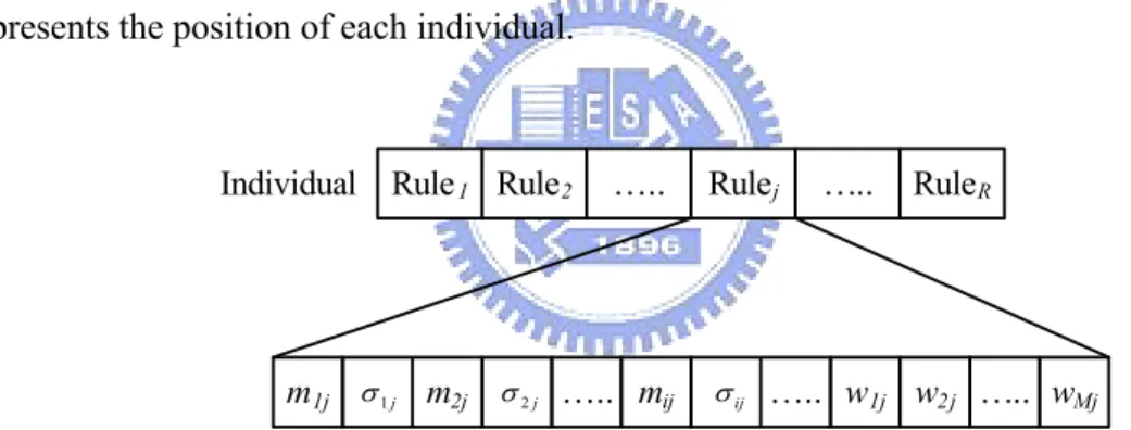
Figure 4.2: Coding a fuzzy rule into an individual in the RSMODE learning algorithm. ...74

Figure 4.3: Structure of the individual in the RSMODE learning algorithm. ...77

Figure 4.4: Illustration of the MODE process for 8-dimensional vector...79

Figure 4.5: A mutation operation in the rule-based symbiotic modified differential evolution. ...81

Figure 4.6: Learning curves of best performance of the FLNFN-RSMODE, FLNFN-RSDE, FLNFN-DE and FLNFN-GA in Example 1. ...83

Figure 4.7: (a) Final regulation performance of FLNFN-RSMODE controller in water bath system. (b) Error curves of the FLNFN-RSMODE controller, FLNFN-RSDE controller, the FLNFN-DE controller, and FLNFN-GA controller. ...83

Figure 4.8: (a) Behavior of FLNFN-RSMODE controller under impulse noise in water bath system. (b) Error curves of FLNFN-RSMODE controller, FLNFN-RSDE controller, the FLNFN-DE controller and FLNFN-GA controller. ...84

Figure 4.9: (a) Behavior of FLNFN-RSMODE controller when a change occurs in the water bath system. (b) Error curves of FLNFN-RSMODE controller, FLNFN-RSDE controller, the FLNFN-DE controller, and FLNFN-GA controller. ...85

Figure 4.10: (a) Tracking of FLNFN-RSMODE controller when a change occurs in the water bath system. (b) Error curves of FLNFN-RSMODE controller, FLNFN-RSDE controller, the FLNFN-DE controller, and FLNFN-GA controller. ...86

Figure 4.11: Learning curves of best performance of the FLNFN-RSMODE, FLNFN-RSDE, FLNFN-DE, and FLNFN-GA in Example 2. ...87

Figure 4.12: Responses of ball and beam system controlled by FLNFN-RSMODE controller (solid curves) and FLNFN-RSDE controller (dotted curves) under four initial conditions. ...88

Figure 4.13: Responses of four states of the ball and beam system under the control of the FLNFN-RSMODE controller. ...88

(19)

Figure 4.15: Learning curves of best performance of the FLNFN-RSMODE, FLNFN-RSDE, FLNFN-DE and FLNFN-GA in Example 3. ...91 Figure 4.16: The moving trajectories of the truck where the solid curves represent the six sets of training trajectories and the dotted curves represent the moving trajectories of the truck under the FLNFN-RSMODE controller. ...91 Figure 4.17: Trajectories of truck, starting at four initial positions under the control of the

(20)

Chapter 1 Introduction

1.1 Motivation

In the field of artificial intelligence, neural networks are essentially low-level computational structures and algorithms that offer good performance when they deal with sensory data. However, it is difficult to understand the meaning of each neuron and each weight in the networks. Generally, fuzzy systems are easy to appreciate because they use linguistic terms and if-then rules. However, they lack the learning capacity to fine-tune fuzzy rules and membership functions. Therefore, neuro-fuzzy networks combine the benefits of neural networks and fuzzy systems to solve many engineering problems. Neuro-fuzzy networks bring the low-level learning and computational power of neural networks into fuzzy systems and give the high-level human-like thinking and reasoning of fuzzy systems to neural networks.

Recently, neuro-fuzzy networks have become popular topics of research, and are applied in many areas, such as prediction, control, identification, recognition, decision-making, etc. Neuro-fuzzy networks have some significant issues including how to design an adaptive neruo-fuzzy network and how to design an effective learning algorithm. Therefore, we propose a functional-link-based neuro-fuzzy network (FLNFN) and its related learning algorithms in this dissertation. The proposed FLNFN model, which combines a neuro-fuzzy

(21)

network with a functional link neural network, is designed to improve the accuracy of functional approximation. Each fuzzy rule that corresponds to a functional link neural network consists of a functional expansion of input variables. The consequent part of the proposed model is a nonlinear combination of input variables. Hence, the local properties of the consequent part in the FLNFN model enable a nonlinear combination of input variables to be approximated more effectively.

Training of the parameters is the main problem in designing a neuro-fuzzy network. Backpropagation (BP) training is commonly adopted to solve this problem. It is a powerful training technique that can be applied to networks with a forward structure. Since the steepest descent approach is used in BP training to minimize the error function, the algorithms may reach the local minima very quickly and never find the global solution. The aforementioned disadvantages lead to suboptimal performance, even for a favorable neuro-fuzzy network topology. Therefore, technologies, that can be used to train the system parameters and find the global solution while optimizing the overall structure, are required. Next, we propose a rule-based symbiotic modified differential evolution (RSMODE) for the proposed FLNFN model. The RSMODE can automatically determine the number of fuzzy rules and generate initial subpopulation. Furthermore, each individual in each subpopulation evolves separately using a modified differential evolution (MODE). The proposed MODE adopts a method to effectively search between the best individual and randomly chosen individuals. Finally, the proposed FLNFN model is applied in various control problems and practical applications. Results of this dissertation demonstrate the effectiveness of the proposed method.

1.2 Literature Survey

Recently, neuro-fuzzy networks [1]-[20] provide the advantages of both neural networks and fuzzy systems, unlike pure neural networks or fuzzy systems alone. Neuro-fuzzy networks

(22)

(NFN) bring the low-level learning and computational power of neural networks into fuzzy systems and give the high-level human-like thinking and reasoning of fuzzy systems to neural networks.

Two typical types of neuro-fuzzy networks are the Mamdani-type and the Takagi-Sugeno-Kang (TSK)-type. For Mamdani-type neuro-fuzzy networks [4]-[6], the minimum fuzzy implication is adopted in fuzzy reasoning. For TSK-type neuro-fuzzy networks (TSK-type NFN) [7]-[10], the consequence part of each rule is a linear combination of input variables. Many researchers [9]-[10] have shown that TSK-type neuro-fuzzy networks offer better network size and learning accuracy than Mamdani-type neuro-fuzzy networks. In the typical TSK-type neuro-fuzzy network, which is a linear polynomial of input variables, the model output is approximated locally by the rule hyper-planes. Nevertheless, the traditional TSK-type neuro-fuzzy network does not take full advantage of the mapping capabilities that may be offered by the consequent part.

Introducing a nonlinear function, especially a neural structure, to the consequent part of the fuzzy rules has yielded the NARA [21] and the CANFIS [22] models. These models [21]-[22] apply multilayer neural networks to the consequent part of the fuzzy rules. Although the interpretability of the model is reduced, the representational capability of the model is markedly improved. However, the multilayer neural network has such disadvantages as slower convergence and greater computational complexity. Therefore, this dissertation uses the functional link neural network (FLNN) [23]-[25] to the consequent part of the fuzzy rules, called a functional-link-based neuro-fuzzy network (FLNFN). The consequent part of the proposed FLNFN model is a nonlinear combination of input variables, which differs from the other existing models [5], [9]-[10]. The FLNN is a single layer neural structure capable of forming arbitrarily complex decision regions by generating nonlinear decision boundaries with nonlinear functional expansion. The FLNN [26] was conveniently used for function approximation and pattern classification with faster convergence rate and less computational

(23)

loading than a multilayer neural network. Moreover, using the functional expansion can effectively increase the dimensionality of the input vector, so the hyper-planes generated by the FLNN will provide a good discrimination capability in input data space.

In addition, training of the parameters is the main problem in designing a neuro-fuzzy network. Backpropagation (BP) training is commonly adopted to solve this problem. It is a powerful training technique that can be applied to networks with a forward structure. Since the steepest descent approach is used in BP training to minimize the error function, the algorithms may reach the local minima very quickly and never find the global solution. The aforementioned disadvantages lead to suboptimal performance, even for a favorable neuro-fuzzy network topology. Therefore, technologies, that can be used to train the system parameters and find the global solution while optimizing the overall structure, are required.

Recent development in genetic algorithms (GAs) has provided a method for neuro-fuzzy system design. Genetic fuzzy systems (GFSs) [27]-[31] hybridize the approximate reasoning of fuzzy systems with the learning capability of genetic algorithms. GAs represent highly effective techniques for evaluating system parameters and finding global solutions while optimizing the overall structure. Thus, many researchers have developed GAs to implement fuzzy systems and neuro-fuzzy systems in order to automate the determination of structures and parameters [32]-[52].

Carse et al. [32] presented a GA-based approach to employ variable length rule sets and simultaneously evolves fuzzy membership functions and relations called Pittsburgh-style fuzzy classifier system. Herrera et al. [33] proposed a genetic algorithm-based tuning approach for the parameters of membership functions used to define fuzzy rules. This approach relied on a set of input-output training data and minimized a squared-error function defined in terms of the training data. Homaifar and McCormick [34] presented a method that simultaneously found the consequents of fuzzy rules and the center points of triangular membership functions in the antecedent using genetic algorithms. Velasco [35] described a

(24)

Michigan approach which generates a special place where rules can be tested to avoid the use of bad rules for online genetic learning. Ishibuchi et al. [36] applied a Michigan-style genetic

fuzzy system to automatically generate fuzzy IF-THEN rules for designing compact fuzzy rule-based classification systems. The genetic learning process proposed is based on the iterative rule learning approach and it can automatically design fuzzy rule-based systems by Cordon et al. [37]. A GA-based learning algorithm called structural learning algorithm in a vague environment (SLAVE) was proposed in [38]. SLAVE used an iterative approach to include more information in the process of learning one individual rule. Furthermore, a very interesting algorithm was proposed by Russo in [39] which attempted to combine all good features of fuzzy systems, neural networks and genetic algorithm for fuzzy model derivation from input-output data. Chung et al. [40] adopted both neural networks and GAs to automatically determine the parameters of fuzzy logic systems. They utilized a feedforward neural network for realizing the basic elements and functions of a fuzzy controller. In [41], a hybrid of evolution strategies and simulated annealing algorithms is employed to optimize membership function parameters and rule numbers which are combined with genetic parameters.

Three main strategies, including Pittsburgh-type, Michigan-type, and the iterative rule learning genetic fuzzy systems, focus on generating and learning fuzzy rules in genetic fuzzy systems. First, the Pittsburgh-type genetic fuzzy system [42] was characterized by using a fuzzy system as an individual in genetic operators. Second, the Michigan-type genetic fuzzy system was used for generating fuzzy rules in [43], where each fuzzy rule was treated as an individual. Thus, the rule generation methods in [43] were referred to as fuzzy classifier systems. Third, the iterative rule learning genetic fuzzy system [44] was adopted to search one adequate rule set for each iteration of the learning process. Moreover, Ishibuchi et al. [45]-[48] proposed genetic algorithms for constructing a fuzzy system consisting of a small number of linguistic rules. Mitra et al. [49]-[52] presented some approaches that exploit the benefits of

(25)

soft computation tools for rule generation.

In the aforementioned literatures, it has been fully demonstrated that GAs are very powerful in searching for the true profile. However, the search is extremely time-consuming, which is one of the basic disadvantages of all GAs. Although the convergence in some special cases can be improved by hybridizing GAs with some local search algorithms, it is achieved at the expense of the versatility and simplicity of the algorithm. Similar to GAs, DE [53]-[55] also belongs to the broad class of evolutionary algorithms, but DE has many advantages such as the strong search ability and the fast convergence ability over GAs or any other traditional optimization approach, especially for real valued problems [55]. Therefore, we propose a rule-based symbiotic modified differential evolution (RSMODE) for the proposed FLNFN model. The RSMODE is to adjust the system parameters and find the global solution while optimizing the overall structure.

1.3 Organization of Dissertation

The overall objective of this dissertation is to develop a novel neuro-fuzzy network and its related learning algorithm. Organization and objectives of each chapter in this dissertation are as follows.

In Chapter 2, we propose a functional-link-based neuro-fuzzy network (FLNFN) structure for nonlinear system control. The proposed FLNFN model uses a functional link neural network (FLNN) to the consequent part of the fuzzy rules. This dissertation uses orthogonal polynomials and linearly independent functions in a functional expansion of the FLNN. Thus, the consequent part of the proposed FLNFN model is a nonlinear combination of input variables. An online learning algorithm, which consists of structure learning and parameter learning, is also presented. The structure learning depends on the entropy measure to determine the number of fuzzy rules. The parameter learning, based on the gradient descent

(26)

method, can adjust the shape of the membership function and the corresponding weights of the FLNN.

In Chapter 3, we present a modified differential evolution (MODE) for the proposed FLNFN model. The proposed MODE learning algorithm adopts an evolutionary learning method to optimize the FLNFN parameters. The MODE algorithm uses a method to effectively search toward the current best individual. Furthermore, the MODE algorithm also provides a cluster-based mutation scheme, which maintains useful diversity in the population to increase the search capability.

In Chapter 4, we propose a rule-based symbiotic modified differential evolution (RSMODE) for the proposed FLNFN model. The proposed RSMODE learning algorithm consists of initialization phase and parameter learning phase. The initialization phase can determine the number of subpopulation which satisfies the fuzzy partition of input variables using the entropy measure. The parameter learning phase combines two strategies including a subpopulation symbiotic evolution and a modified differential evolution. The RSMODE can automatically generate initial subpopulation and each individual in each subpopulation evolves separately using a modified differential evolution. We also compare our method with other methods in the literature early. Finally, conclusions and future works are summarized in the last section.

(27)

Chapter 2 A Functional-Link-Based Neuro-Fuzzy Network

In this chapter, a functional-link-based neuro-fuzzy network (FLNFN) model is presented for nonlinear system control. The FLNFN model, which combines a neuro-fuzzy network with a functional link neural network (FLNN), is designed to improve the accuracy of functional approximation. Each fuzzy rule that corresponds to a FLNN consists of a functional expansion of input variables. The orthogonal polynomials and linearly independent functions are adopted as functional link neural network bases. An online learning algorithm, consisting of structure learning and parameter learning, is proposed to construct the FLNFN model automatically. The structure learning algorithm determines whether or not to add a new node which satisfies the fuzzy partition of input variables. Initially, the FLNFN model has no rules. The rules are automatically generated from training data by entropy measure. The parameter learning algorithm is based on back-propagation to tune the free parameters in the FLNFN model simultaneously to minimize an output error function.

2.1 Structure of Functional-Link-Based Neuro-Fuzzy Network

This section describes the structure of functional link neural networks and the structure of the FLNFN model. In functional link neural networks, the input data usually incorporate high order effects and thus artificially increase the dimensions of the input space using a functional

(28)

expansion. Accordingly, the input representation is enhanced and linear separability is achieved in the extended space. The FLNFN model adopted the functional link neural network generating complex nonlinear combination of input variables to the consequent part of the fuzzy rules. The rest of this section details these structures.

2.1.1 Functional Link Neural Networks

The functional link neural network is a single layer network in which the need for hidden layers is removed. While the input variables generated by the linear links of neural networks are linearly weighted, the functional link acts on an element of input variables by generating a set of linearly independent functions (i.e., the use of suitable orthogonal polynomials for a functional expansion), and then evaluating these functions with the variables as the arguments. Therefore, the FLNN structure considers trigonometric functions. For example, for a two-dimensional input _[_x_,_x _]T

2 1

=

X , the enhanced input is obtained using trigonometric functions in _[_x _,_sin₍ _x₎_,_cos₍ _x₎_,...,_x _,_sin₍ _x ₎_,_cos₍ _x ₎_,..._]T

2 2 2 1 1 1 π π π π =

Φ . Thus, the input

variables can be separated in the enhanced space [23]. In the FLNN structure with reference to Fig. 2.1, a set of basis functions Φ and a fixed number of weight parameters W represent fW(x). The theory behind the FLNN for multidimensional function approximation has been discussed elsewhere [24] and is analyzed below.

x1 x2

Functional

Expansion

. . . xN . . . . . . 1 φ 2 φ M φ

∑

1 ˆy 2 ˆy m yˆ X W Yˆ Figure 2.1: Structure of FLNN.

(29)

properties; 1) φ1 =1, 2) the subset

M k j ={φ ∈Β}k 1=

Β is a linearly independent set, meaning that if

∑

M₌ =

k 1wkφk 0, then wk =0 for all k=1,2,...,M , and 3)

[

∑

=

]

<∞ 2 1 1 2 / j k k A j sup φ . Let M k}k 1 { ₌ = φ

Β be a set of basis functions to be considered, as shown in Fig. 2.1. The FLNN comprises M basis functions {φ1,φ2,...,φ_M}∈Β_M. The linear sum of the jth node is

given by

∑

= = M k k kj j w ( ) yˆ 1 X φ (2.1) where _X_∈_Α_⊂_ℜN_, T N x x x, ,..., ] [ ₁ ₂ =

X is the input vector and T jM j

j

j =[w1,w 2,...,w ]

W is

the weight vector associated with the jth output of the FLNN. ˆy denotes the local output of _j

the FLNN structure and the consequent part of the jth fuzzy rule in the FLNFN model. Thus, Eq.(2.1) can be expressed in matrix form as yˆj =WjΦ, where

T N x , ... x x), ( ), ( )] ( [φ1 φ2 φ = Φ

is the basis function vector, which is the output of the functional expansion block. The

m-dimensional linear output may be given by Yˆ =WΦ, where T

m yˆ ... yˆ yˆ ˆ _[ _, _, _, _] 2 1 = Y , m

denotes the number of functional link bases, which equals the number of fuzzy rules in the FLNFN model, and W is a (m×M)-dimensional weight matrix of the FLNN given by

T

] ,..., ,

[w1 w2 wM

W= . In the FLNFN model, the corresponding weights of functional link bases do not exist in the initial state, and the amount of the corresponding weights of functional link bases generated by the online learning algorithm is consistent with the number of fuzzy rules. Section 3 details the online learning algorithm.

2.1.2 Structure of the FLNFN Model

This subsection describes the FLNFN model, which uses a nonlinear combination of input variables (FLNN). Each fuzzy rule corresponds to a sub-FLNN, comprising a functional link. Figure 2.2 presents the structure of the proposed FLNFN model.

(30)

The FLNFN model realizes a fuzzy if-then rule in the following form.

Rule-j: IFx₁isA₁_jandx₂is A₂_j...andx_iisA_ij...andx_NisA_Nj

M Mj j j M k k kj j w w w w y φ φ φ φ + + + = =

∑

= ... ˆ THEN 2 2 1 1 1 (2.2)

where xi and yˆ are the input and local output variables, respectively; A_j ij is the linguistic

term of the precondition part with Gaussian membership function; N is the number of input variables; wkj is the link weight of the local output; φ_k is the basis trigonometric function of

input variables; M is the number of basis function, and Rule-j is the jth fuzzy rule.

x1 x2

Functi

onal

Expansion

x1 x2 y w11 w21 wM1 . . . . . . . . . . . . . . .

Layer 1 Layer 2 Layer 3 Layer 4 Layer 5

Normalization

1 ˆy 2 ˆy 3 ˆy 1 φ 2 φ M φ ∑ ∑ ∑

Figure 2.2: Structure of proposed FLNFN model.

The operation functions of the nodes in each layer of the FLNFN model are now described. In the following description, u(l)_{denotes the output of a node in the lth layer.}

(31)

No computation is performed in layer 1. Each node in this layer only transmits input values to the next layer directly:

i

i x

u(1) = _{. (2.3)} Each fuzzy set Aij is described here by a Gaussian membership function. Therefore, the

calculated membership value in layer 2 is

        − − = ₂ 2 1 2 [ ] ij ij ) ( i ) ( ij m u exp u σ (2.4)

where mij and σij are the mean and variance of the Gaussian membership function,

respectively, of the jth term of the ith input variable xi.

Nodes in layer 3 receive one-dimensional membership degrees of the associated rule from the nodes of a set in layer 2. Here, the product operator described above is adopted to perform the precondition part of the fuzzy rules. As a result, the output function of each inference node is

∏

= i ij j u u(3) (2)_(2.5) where the

∏

i ij

u(2) _{of a rule node represents the firing strength of its corresponding rule.}

Nodes in layer 4 are called consequent nodes. The input to a node in layer 4 is the output from layer 3, and the other inputs are calculated from a functional link neural network, as shown in Fig. 2.2. For such a node,

∑

= ⋅ = M k k kj j j u w u 1 ) 3 ( ) 4 ( _φ _(2.6)

where wkj is the corresponding link weight of functional link neural network and φk is the

functional expansion of input variables. The functional expansion uses a trigonometric polynomial basis function, given by

[

φ₁ φ₂ φ₃ φ₄ φ₅ φ₆

]

=

[

x1sin(π x1) cos(π x1 )x2sin(π x2 )cos(π x2)

]

for two-dimensional input variables. Therefore,

(32)

Moreover, the output nodes of functional link neural network depend on the number of fuzzy rules of the FLNFN model.

The output node in layer 5 integrates all of the actions recommended by layers 3 and 4 and acts as a defuzzifier with,

∑

= = = = = = = ₌       = = = _R j ) ( j R j j ) ( j R j ) ( j R j M k k kj ) ( j R j ) ( j R j ) ( j ) ( u yˆ u u w u u u u y 1 3 1 3 1 3 1 1 3 1 3 1 4 5 φ (2.7)

where R is the number of fuzzy rules, and y is the output of the FLNFN model.

As described above, the number of tuning parameters for the FLNFN model is known to be (2+3×P)×N×R, where N, R and P denote the number of inputs, existing rules, and outputs, respectively. The proposed FLNFN model can be demonstrated to be a universal uniform approximation by Stone-Weierstrass theorem [56] for continuous functions over compact sets. The detailed proof is given in the Appendix.

2.2 Learning Algorithms of the FLNFN Model

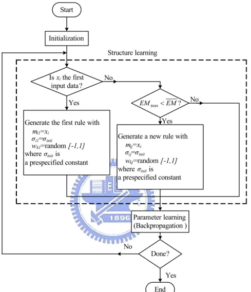
This section presents an online learning algorithm for constructing the FLNFN model. The proposed learning algorithm comprises a structure learning phase and a parameter learning phase. Figure 2.3 presents flow diagram of the learning scheme for the FLNFN model. Structure learning is based on the entropy measure used to determine whether a new rule should be added to satisfy the fuzzy partitioning of input variables. Parameter learning is based on supervised learning algorithms. The back-propagation algorithm minimizes a given cost function by adjusting the link weights in the consequent part and the parameters of the membership functions. Initially, there are no nodes in the network except the input-output nodes, i.e., there are no any nodes in the FLNFN model. The nodes are created automatically as learning proceeds, upon the reception of online incoming training data in the structure and parameter learning processes. The rest of this section details the structure learning phase and

(33)

the parameter learning phase. Finally in this section, the stability analysis of the FLNFN model based on the Lyapunov approach is performed the convergence property.

Start

Initialization

Is xi the first

input data?

Generate the first rule with

mi1=xi

σi1=σinit

wk1=random [-1,1]

where σinit is

a prespecified constant

Generate a new rule with

mij=xi σij=σinit wkj=random [-1,1] where σinit is a prespecified constant Yes No Yes No Done? End Yes No Parameter learning (Backpropagation ) ? max EM EM < Structure learning

Figure 2.3: Flow diagram of the structure/parameter learning for the FLNFN model.

2.2.1 Structure Learning Phase

The first step in structure learning is to determine whether a new rule from should be extracted the training data and to determine the number of fuzzy sets in the universal of discourse of each input variable, since one cluster in the input space corresponds to one potential fuzzy logic rule, in which m and ij σij represent the mean and variance of that

(34)

the degree to which the incoming pattern belongs to the corresponding cluster. Entropy measure between each data point and each membership function is calculated based on a similarity measure. A data point of closed mean will has lower entropy. Therefore, the entropy values between data points and current membership functions are calculated to determine whether or not to add a new rule. For computational efficiency, the entropy measure can be calculated using the firing strength from (2)

ij u as follow;

∑

= − = N i ij ij j D D EM 1 2 log (2.8) where ₌_exp

( )

(2)−1 ij ij u

D and EMj∈[0,1]. According to Eq. (2.8), the measure is used to generate a new fuzzy rule and new functional link bases for new incoming data is described as follows. The maximum entropy measure

j R j EM EM T ) ( 1 max = _≤max_≤ (2.9)

is determined, where R(t) is the number of existing rules at time t. If EM_max ≤ EM, then a

new rule is generated, where EM∈[0,1] is a prespecified threshold that decays during the learning process.

In the structure learning phase, the threshold parameter EM is an important parameter. The threshold is set to between zero and one. A low threshold leads to the learning of coarse clusters (i.e., fewer rules are generated), whereas a high threshold leads to the learning of fine clusters (i.e., more rules are generated). If the threshold value equals zero, then all the training data belong to the same cluster in the input space. Therefore, the selection of the threshold value EM will critically affect the simulation results. As a result of our extensive experiments and by carefully examining the threshold value EM , which uses the range [0, 1], we concluded that the relationship between threshold value EM and the number of input variables. Accordingly, EM is defined as 0.26-0.3 times of the number of input variables.

(35)

variance to the new membership function and the corresponding link weight for the consequent part. Since the goal is to minimize an objective function, the mean, variance and weight are all adjustable later in the parameter learning phase. Hence, the mean, variance and weight for the new rule are set as follows;

i R ij x m( (t+1)) = _(2.10) init R ij t σ σ( (+1)) = _(2.11) ] 1 , 1 [ ) ( (+1) =_random− wRt kj (2.12)

where xi is the new input and σ_init is a prespecified constant. The whole algorithm for the

generation of new fuzzy rules and fuzzy sets in each input variable is as follows. No rule is assumed to exist initially exist:

Step 1: IF xi is the first incoming pattern THEN do

{Generate a new rule

with mean mi1=xi, variance σi1=σinit, weight wk1=random[-1, 1]

where σinit is a prespecified constant.

}

Step 2: ELSE for each newly incoming xi, do

{Find _j R j EM EM t ) ( 1 max = max_≤ _≤ IF EMmax ≥EM do nothing ELSE {R(t+1) = R(t) +1

generate a new rule

with mean m_iR₍_t₊₁₎ =x_i, variance _iR _init ) t

( σ

σ ₊₁ = , weight wkR₍_t+1₎ =random[−1,1]

(36)

}

2.2.2 Parameter Learning Phase

After the network structure has been adjusted according to the current training data, the network enters the parameter learning phase to adjust the parameters of the network optimally based on the same training data. The learning process involves determining the minimum of a given cost function. The gradient of the cost function is computed and the parameters are adjusted with the negative gradient. The back-propagation algorithm is adopted for this supervised learning method. When the single output case is considered for clarity, the goal to minimize the cost function E is defined as

) ( 2 1 )] ( ) ( [ 2 1 ) (_t _y_t _y _t 2 _e2 _t E ₌ ₋ d ₌ _(2.13)

where yd(t) is the desired output and y(t) is the model output for each discrete time t. In each training cycle, starting at the input variables, a forward pass is adopted to calculate the activity of the model output y(t).

When the back-propagation learning algorithm is adopted, the weighting vector of the FLNFN model is adjusted such that the error defined in Eq. (2.13) is less than the desired threshold value after a given number of training cycles. The well-known back-propagation learning algorithm may be written briefly as

      ∂ ∂ − + = ∆ + = + ) ( ) ( ) ( ) ( ) ( ) 1 ( t W t E t W t W t W t W η (2.14) where, in this case, η and W represent the learning rate and the tuning parameters of the FLNFN model, respectively. Let _W₌_[_m_,_σ_,_w_]T_{be the weighting vector of the FLNFN}

model. Then, the gradient of error E(.) in Eq. (2.13) with respect to an arbitrary weighting vector W is W t y t e W t E ∂ ∂ = ∂ ∂ () ) ( ) ( . (2.15) Recursive applications of the chain rule yield the error term for each layer. Then the

(37)

parameters in the corresponding layers are adjusted. With the FLNFN model and the cost function as defined in Eq. (2.13), the update rule for wj can be derived as follows;

) ( ) ( ) 1 (t w t w t w_kj + = _kj +∆ _kj (2.16) where         ⋅ ⋅ − = ∂ ∂ − =

∑

= R j j k j w kj w kj u u e w E t w 1 ) 3 ( ) 3 ( ) ( φ η η ∆ .

Similarly, the update laws for mij, and σ_ij are

) ( ) ( ) 1 (t m t m t mij + = ij +∆ ij (2.17) ) ( ) ( ) 1 (t ij t ij t ij σ ∆σ σ + = + (2.18) where         − ⋅         ⋅ ⋅ − = ∂ ∂ − =

∑

= 2 ) 1 ( 1 ) 3 ( ) 4 ( ₂₍ ₎ ) ( ij ij i R j j j m ij m ij m u u u e m E t m σ η η ∆         − ⋅         ⋅ ⋅ − = ∂ ∂ − =

∑

= 3 2 ) 1 ( 1 ) 3 ( ) 4 ( ₂₍ ₎ ) ( ij ij i R j j j ij ij m u u u e E t σ η σ η σ ∆ σ σ

where ηw, ηm and ησ are the learning rate parameters of the weight, the mean, and the

variance, respectively. In this dissertation, both the link weights in the consequent part and the parameters of the membership functions in the precondition part are adjusted by using the back-propagation algorithm. Recently, many researchers [10], [57] tuned the consequent parameters using either least mean squares (LMS) or recursive least squares (RLS) algorithms to obtain optimal parameters. However, they still used the back-propagation algorithm to

(38)

adjust the precondition parameters.

2.2.3 Convergence Analysis

The selection of suitable learning rates is very important. If the learning rate is small, convergence will be guaranteed. In this case, the speed of convergence may be slow. However, the learning rate is large, and then the system may become unstable. The Appendix derives varied learning rates, which guarantee convergence of the output error based on the analyses of a discrete Lyapunov function, to train the FLNFN model effectively. The convergence analyses in this dissertation are performed to derive specific learning rate parameters for specific network parameters to ensure the convergence of the output error [58]-[59]. Moreover, the guaranteed convergence of output error does not imply the convergence of the learning rate parameters to their optimal values. The following simulation results demonstrate the effectiveness of the online learning FLNFN model based on the proposed delta adaptation law and varied learning rates.

2.3 Experimental Results

This dissertation demonstrated the performance of the FLNFN model for nonlinear system control. This section simulates various control examples and compares the performance of the FLNFN model with that of other models. The FLNFN model is adopted to design controllers in four simulations of nonlinear system control problems - water bath temperature control system [60], control of a bounded input bounded output (BIBO) nonlinear plant [58], control of the ball and beam system [61], and multi-input multi-output (MIMO) plant control [62].

Example 1: Control of Water Bath Temperature System

(39)

system according to, C T t y Y C t u dt t dy R ) ( ) ( ) ( ₌ ₊ 0− _(2.19)

where y(t) is the output temperature of the system in C° ; u(t) is the heat flowing into the system; Y is room temperature; C is the equivalent thermal capacity of the system, and T₀ R is

the equivalent thermal resistance between the borders of the system and the surroundings.

TR and C are assumed to be essentially constant, and the system in Eq.(2.19) is rewritten

in discrete-time form to some reasonable approximation. The system

0 40 ) ( 5 . 0 ( ) [1 ] 1 ) 1 ( ) ( ) 1 ( u k e y e e k y e k y Ts k y Ts Ts α α α α δ − − − − ₊ ₋ + − + = + (2.20) is obtained, where α and δ are some constant values of TR and C. The system parameters

used in this example are _α₌₁_.₀₀₁₅_e−4_, _δ ₌₈_.₆₇₉₇₃_e−3_and 0

Y =25.0( C° ), which were

obtained from a real water bath plant considered elsewhere [60]. The plant input u(k) is limited to 0 and 5V, and the sampling period is Ts=30 second.

The conventional online training scheme is adopted for online training. Figure 2.4 presents a block diagram for the conventional online training scheme. This scheme has two phases - the training phase and the control phase. In the training phase, the switches S1 and S2 are connected to nodes 1 and 2, respectively, to form a training loop. In this loop, we can define a training data with input vector I(k)=[y_p(k+1) y_p(k)] and desired output u(k), where the input vector of the FLNFN controller is the same as that used in the general inverse modeling [63] training scheme. In the control phase, the switches S1 and S2 are connected to nodes 3 and 4, respectively, forming a control loop. In this loop, the control signal uˆ k( ) is generated according to the input vector I'(k)=[y_ref(k+1) y_p(k)], where y is the plant _p

output and y is the reference model output. _ref

(40)

simulated system described in Eq. (2.20), using the online training scheme for the FLNFN controller. The 120 training patterns are selected based on the input-outputs characteristics to cover the entire reference output. The temperature of the water is initially 25°c, and rises progressively when random input signals are injected. After 10000 training iterations, four fuzzy rules are generated. The obtained fuzzy rules are as follows.

Rule-1: IFx1isµ(32.416,11.615)andx2isµ(27.234,7.249) ) x cos( ) x sin( . x . ) x cos( . ) x sin( . x yˆ 2 2 2 1 1 1 1 35.204 799 41 026 17 546 34 849 74 32.095 THEN π π π π + − − − + = Rule-2: IFx1isµ(34.96,9.627)andx2isµ(46.281,13.977) ) x cos( ) x sin( x ) x cos( ) x sin( x yˆ 2 2 2 1 1 1 2 70.946 61.827 52.923 77.705 11.766 21.447 THEN π π π π + − − − + = Rule-3: IFx₁isµ(62.771,6.910)andx₂isµ(62.499,15.864) ) x cos( ) x sin( x ) x cos( ) x sin( x yˆ 2 2 2 1 1 1 3 103.33 36.752 40.322 46.359 10.907 25.735 THEN π π π π + + − − − = Rule-4: IFx₁isµ(79.065,8.769)andx₂isµ(64.654,9.097) ) x cos( ) x sin( x ) x cos( ) x sin( x yˆ 2 2 2 1 1 1 4 34.838 61.065 5.8152 57.759 37.223 46.055 THEN π π π π + + − − − = yp(k+1) yref(k+1) yp(k+1) 1 3 S1 Z-1 2 4 S2 ) ( ˆ k u ) (k u + Plant Z-1 – FLNFN Controller

Figure 2.4: Conventional online training scheme.

This dissertation compares the FLNFN controller to the proportional-integral-derivative (PID) controller [64], the manually designed fuzzy controller [1], the functional link neural network [25] and the TSK-type neuro-fuzzy network (TSK-type NFN) [9]. Each of these controllers is applied to the water bath temperature control system. The performance measures include the set-points regulation, the influence of impulse noise, and a large parameter

以函數鏈結為基礎之類神經模糊網路及其應用

國

國

國

國

立

立

立

立

交

交

交

交

通

通

通

通

大

大

大

大

學

學

學

學

電機與控制工程學系

電機與控制工程學系

電機與控制工程學系

電機與控制工程學系

博

博

博

博

士

士

士

士

論

論

論

論

文

文

文

文

以函數鏈結為基礎之類神經模糊網路及其應用

以函數鏈結為基礎之類神經模糊網路及其應用

以函數鏈結為基礎之類神經模糊網路及其應用

以函數鏈結為基礎之類神經模糊網路及其應用

A Functional-Link-Based Neuro-Fuzzy Network and Its Applications

研

研

研

研 究

究

究 生

究

生

生

生：

：

：

：陳政宏

陳政宏

陳政宏

陳政宏

指導教授

指導教授

指導教授

指導教授：

：

：

：林進燈

林進燈

林進燈

林進燈

中

中

中

中 華

研究

究生

中華

華民

民國

國九

九十

十七

七年

年七

七月

研究生：陳政宏

指導教授：林進燈博士

國立交通大學

電機與控制工程學系

博士論文