Theoretical Formulation and Simulation of Electronic Sum-Frequency Generation Spectroscopy

(1)

Theoretical Formulation and Simulation of Electronic Sum-Frequency

Generation Spectroscopy

Chih-Kai Lin,*

,†

Michitoshi Hayashi,

†

and Sheng Hsien Lin

‡,§

†_{Center for Condensed Matter Sciences, National Taiwan University, Taipei, Taiwan 106, Republic of China} ‡_{Department of Applied Chemistry, National Chiao Tung University, Hsinchu, Taiwan 30010, Republic of China} §_{Institute of Atomic and Molecular Sciences, Academia Sinica, Taipei, Taiwan 10617, Republic of China}

ABSTRACT: Sum-frequency generation (SFG) spectroscopy

is a powerful tool for not only identifying molecular species but also analyzing orientation conﬁgurations on a surface/ interface. In this Article, we presented reformulation of the theoretical framework of electronic SFG spectroscopy, the signal of which could be greatly enhanced by tuning one or two incident beam frequencies resonant with electronic excited states. Simulated electronic SFG spectra resonant at the sum frequency of a pair of coumarin-derivative pH-indicator surfactant molecules, 4-methyl-7-hydroxycoumarin and its anionic counterpart (MHC/MHC−), ﬂoating on the water surface were carried out as a demonstration.

I. INTRODUCTION

Sum-frequency generation (SFG) spectroscopy, due to its surface- and interface-speciﬁcity, has become a powerful tool in resolving surface and interfacial molecular conﬁgurations in the last two decades. This second-order nonlinear optical technique can, by tuning incident beam frequencies resonant with molecular vibrational and/or electronic excitations, detect not only species but also molecular orientation distributions on the sample surface/interface.1−5 Pioneered by Shen’s group, vibrational sum-frequency generation (VSFG) spectroscopy has been applied in examining molecular structures of ice and liquid water surface,4,6 and, with phase-sensitive detection, it has revealed the topology of hydrogen bonding in the topmost layers of liquid water.7−11 VSFG has also been applied to analyze molecular orientations in other systems such as organic polymers immersed in water or adsorbed on a solid substrate.12−14 In the theoretical aspect, a susceptibility approach combined with Euler angle transformation has been established and applied to interpret these VSFG spectra.15−17

In addition to VSFG, Tahara and co-workers have recently made heterodyne-detected electronic sum-frequency generation (ESFG) spectroscopy applicable.18−20In their experiments, two visible/near-infrared beams were guided to the sample where the sum frequency was tuned resonant with an electronic state. By this means, the orientation distribution of surfactant molecules floating on water surface could be resolved, and, furthermore, the pH value of water surface was claimed.21−23It should be noticed that, however, a comprehensive theoretical framework to interpret these beautiful experimental results is still in demand. In this Article, we shall examine the mathematical formulation of ESFG spectroscopy and derive specific descriptions to different resonance and off-resonance

cases. We shall also simulate the ESFG spectra of 4-methyl-7-hydroxycoumarin and its phenoxide anionic counterpart (noted as MHC/MHC−), which is a simpler analogue to 4-hectadecyl-7-hydroxycoumarin (noted as HHC/HHC−), a coumarin-based pH-indicator reported previously,23−25 as a demonstration of our theoretical model.

II. THEORIES

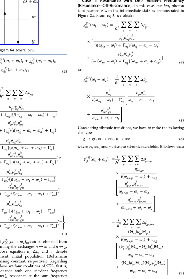
The detailed mathematical framework of SFG has been discussed in the literature,1−3,16 and brief illustrations for specific resonance conditions are given below. For a general case, one can consider an energy level diagram for SFG as shown in Figure 1, where g, m, and n denote the initial, intermediate, andfinal state manifolds, and ω₁andω₂represent the angular frequencies of the two incident beams. By definition, the microscopic second-order SFG susceptibility, χijl(2)(ω1 + ω2), of a molecule is the proportional constant

relating polarization and electricﬁelds:

∑ ∑

ω ω χ ω ω ω ω ⃗ + = + P_i ( ) ( )E ( )E ( ) j k ijk j k (2) 1 2 (2) 1 2 1 1 2 2 (1) where i, j, and k are Cartesian coordinates. It can be written explicitly as

Received: August 7, 2013

Revised: October 12, 2013

Published: October 14, 2013

(2)

χ ω ω χ ω ω χ ω ω χ ω ω + = + + + + + ( ) ( ) ( ) ( )

ijk ijk ijk

ijk (2) 1 2 (2) 1 2 I (2) 1 2 II (2) 1 2 III ₍₂₎ where

∑ ∑ ∑

χ ω ω ρ μ μ μ ω ω ω ω ω μ μ μ ω ω ω ω ω μ μ μ ω ω ω ω ω μ μ μ ω ω ω ω ω μ μ μ ω ω ω ω ω μ μ μ ω ω ω ω ω μ μ μ ω ω ω ω ω μ μ μ ω ω ω ω ω + = ℏ Δ × − + Γ − − + Γ + − + Γ − − + Γ + + + Γ + + + Γ + + + Γ + + + Γ * − − + Γ − − + Γ + − + Γ − − + Γ − + + Γ + + + Γ + + + Γ + + + Γ * ⎪ ⎪ ⎪ ⎪ ⎧ ⎨ ⎩ ⎫ ⎬ ⎭ i i i i i i i i i i i i i i i i i ( ) [ { ( ) }{ ( ) } { ( ) }{ ( ) }] [ { ( ) }{ ( ) } { ( ) }{ ( ) }] [ { ( ) }{ ( ) } { ( ) }{ ( ) }] [ { ( ) }{ ( ) } { ( ) }{ ( ) }] ijk g m n gm gn i mg j nm k mg mg ng ng gn i nm j mg k mg mg ng ng ng i mg j nm k mg mg ng ng ng i nm j mg k mg mg ng ng mn i gm j ng k gm mg nm nm mn i ng j gm k gm mg nm nm nm i gm j ng k gm mg nm nm nm i ng j gm k gm mg nm nm (2) 1 2 I 2 2 1 1 2 2 1 2 1 1 2 2 1 2 1 1 2 2 1 2 1 1 2 2 1 2 (3) andχ_ijk(2)₍_ω

1+ω2)IIandχ(2)ijk(ω1+ω2)IIIcan be obtained from

χijk(2)(ω1+ω2)Iby performing the exchanges n↔ m and n ↔ g,

respectively. In the above equation μ, Δρ, and Γ denote transition dipole moment, initial population (Boltzmann distribution), and dephasing constant, respectively. Regarding resonance conditions, there are four conditions of SFG, that is, double resonance, resonance with one incident frequency (resonance−oﬀ-resonance), resonance at the sum frequency

(oﬀ-resonance−resonance), and both oﬀ-resonance. For

example, the resonance−oﬀ-resonance case means that the

ℏω1 photon is in resonance with the g→ m transition, while

the ℏω2 photon is not resonant with the n state. We shall

discuss cases with at least one resonance, which are applied in experiments, in the following paragraphs.

Case 1: Resonance with One Incident Frequency (Resonance−Oﬀ-Resonance). In this case, the ℏω₁photon is in resonance with the intermediate state as demonstrated in Figure 2a. From eq 3, we obtain:

∑ ∑ ∑

χ ω ω ρ μ μ μ ω ω ω ω ω μ μ μ ω ω ω ω ω + = ℏ Δ × − + Γ − − + − + + Γ + + i i i ( ) [ { ( ) }( ) { ( ) }( )] ijk g m n gm gn i mg j nm k mg mg ng nm i mg j gn k gm mg nm (2) 1 2 2 1 1 2 1 1 2 (4) or

∑ ∑ ∑

χ ω ω ρ μ ω ω μ μ ω ω ω μ μ ω ω ω + = ℏ Δ × − + Γ − − + + + ⎡ ⎣ ⎢ ⎢ ⎤ ⎦ ⎥ ⎥ i i ( ) ( ) ijk g m n gm mg j mg mg gn i nm k ng nm i gn k nm (2) 1 2 2 1 1 2 1 2 ₍₅₎

Considering vibronic transitions, we have to make the following changes:

→ → →

g gv m, mu n, nw (6)

where gv, mu, and nw denote vibronic manifolds. It follows that:

∑ ∑ ∑

χ ω ω ρ μ ω ω μ μ ω ω ω μ μ ω ω ω ρ μ ω ω μ μ ω ω ω μ μ ω ω ω + = ℏ Δ × − + Γ − − + + + = ℏ Δ × ⟨Θ | |Θ ⟩ − + Γ ⟨Θ | |Θ ⟩⟨Θ | |Θ ⟩ − − + ⟨Θ | |Θ ⟩⟨Θ | |Θ ⟩ + + ⎡ ⎣ ⎢ ⎢ ⎤ ⎦ ⎥ ⎥ ⎡ ⎣ ⎢ ⎢ ⎤ ⎦ ⎥ ⎥ i i i i ( ) ( ) ( ) ijk v u nw gv mu mu gv j mu gv mg gv nw i nw mu k nw gv nw mu i gv nw k nw mu v u nw gv mu mu mg j gv mu gv mg gv gn i nw nw nm k mu ng nw nm i mu gv gn k nw nm (2) 1 2 2 , , , 1 , , , 1 2 , , , 1 2 2 , , 1 1 2 1 2 ₍₇₎

Here,Θ denotes the nuclear (vibrational) wave function. Note that the Placzek approximation,ωnw,gv≈ ωngandωnw,mu≈ ωnm,

(3)

is applied. By using the closure relation over nw states, ∑w|Θnw⟩⟨Θnw| = 1, it is found that:

∑ ∑

χ ω ω ρ μ α ω ω + = ℏ Δ ⟨Θ | |Θ ⟩⟨Θ | |Θ ⟩ − + Γ i i ( ) ( ) ijk v u gv mu mu mgj gv gv gmik mu mu gv mg (2) 1 2 2 , , 1 (8)

whereαgmik is the polarizability-like two-photon transition matrix

element deﬁned by

∑

α μ μ ω ω ω μ μ ω ω ω ω = − − + + + + ⎡ ⎣ ⎢ ⎢ ⎤ ⎦ ⎥ ⎥ gmik n gn i nm k ng nm i gn k ng gm 1 2 1 2 (9) The real and imaginary parts of the second-order susceptibility are

∑ ∑

χ ω ω ρ ω ω μ α ω ω + = ℏ Δ − ⟨Θ | |Θ ⟩⟨Θ | |Θ ⟩ − + Γ Re[ ( )] 1 ( ) ( ) ijk v u gv mu mu gv mu mg j gv gv gm ik mu mu gv mu gv (2) 1 2 2 , , 1 , 1 2 , 2 (10a)

∑ ∑

χ ω ω ρ μ α ω ω + = ℏ Δ Γ ⟨Θ | |Θ ⟩⟨Θ | |Θ ⟩ − + Γ Im[ ( )] 1 ( ) ijk v u gv mu mu gv mu mg j gv gv gm ik mu mu gv mu gv (2) 1 2 2 , , , 1 2 , 2 (10b) respectively. In the Condon approximation:

∑ ∑

χ ω ω μ α ρ ω ω ω ω + = ℏ Δ − |⟨Θ |Θ ⟩| − + Γ Re[ ( )] 1 ( ) ( ) ijk mg j gmik v u gv mu mu gv gv mu mu gv mu gv (2) 1 2 2 , , 1 2 , 12 2 , (11a) and

∑ ∑

χ ω ω μ α ρ ω ω + = ℏ Δ Γ |⟨Θ |Θ ⟩| − + Γ Im[ ( )] 1 ( ) ijk mg j gm ik v u gv mu mu gv gv mu mu gv mu gv (2) 1 2 2 , , 2 , 12 2 , (11b)

The two parts relate to each other by the Kronig−Kramers transform. Equation 11b indicates that, supposing the variations of μ and α with respect to ω are negligible, the band-shape function of Im[χijl(2)(ω1 + ω2)] is exactly the same as the

conventional electronic absorption spectrum:

∑ ∑

ρ ω ω = Δ Γ |⟨Θ |Θ ⟩| − + Γ F ( ) v u gv mu mu gv gv mu mu gv mu gv , , 2 , 1 2 , 2 (12a) or, by assuming a Gaussian inhomogeneous broadening with the center at ω̅_mu,gv and a deviation of σ_mu,gv for each corresponding vibrational mode:8

∫

∑ ∑

ρ ω ω ω ω ω σ = Δ Γ |⟨Θ |Θ ⟩| − + Γ × − − ̅ ⎡ ⎣ ⎢ ⎢ ⎤ ⎦ ⎥ ⎥ F d ( ) exp ( ) v u gv mu mu gv mu gv gv mu mu gv mu gv mu gv mu gv mu gv , , , 2 , 12 2 , , , 2 , 2 (12b) for the g→ m transition. However, the transition intensity is determined by the electronic matrix elementμ_mgj _α

gm

ik _{in ESFG}

spectroscopy, rather than |μ⃗mg|2 in conventional electronic

absorption spectroscopy.

Note that this resonance condition is widely applied in VSFG as well. In the vibrational case, the resonance occurs in the same electronic state, that is, m = g, and hence in eq 10, the transition matrix elements become permanent dipole moment, μ_gg, and polarizability,αgg, of the ground state. The two quantities can

Figure 2. Energy level diagrams for diﬀerent resonant ESFG

conditions: (a) resonance with one incident frequency (resonance− oﬀ-resonance), (b) resonance at the sum frequency (oﬀ-resonance− resonance), and (c) double resonance.

(4)

be expanded in the power series of vibrational mode Q, and an active mode must have (∂μgg/∂Q)0(∂αgg/∂Q)0≠ 0 according to

IR and Raman selection rules. The details can be found in the literature.2−6

Case 2: Resonance at the Sum-Frequency (O

ﬀ-Resonance−Resonance). We next consider resonance at

the sum frequency as shown in Figure 2b. From eq 3, weﬁnd:

∑ ∑ ∑

χ ω ω ρ μ ω ω ω μ μ ω ω μ μ ω ω + = ℏ Δ − − + Γ − + − ⎡ ⎣ ⎢ ⎢ ⎤ ⎦ ⎥ ⎥ i i ( ) ( ) ijk g m n gm gn i ng ng mg j nm k mg nm j mg k mg (2) 1 2 2 1 2 1 2 ₍₁₃₎

In terms of vibronic states, we ﬁnd that (with the Placzek approximation,ωmu,gv≈ ωmg):

∑ ∑ ∑

χ ω ω ρ μ ω ω ω μ μ ω ω μ μ ω ω + = ℏ Δ ⟨Θ | |Θ ⟩ − − + Γ × ⟨Θ | |Θ ⟩⟨Θ | |Θ ⟩ − +⟨Θ | |Θ ⟩⟨Θ | |Θ ⟩ − ⎡ ⎣ ⎢ ⎢ ⎤ ⎦ ⎥ ⎥ i i ( ) ( ) ijk v w mu gv mu gv gn i nw nw gv nw gv mu mg j gv nw nm k mu mg nw nm j mu mu mg k gv mg (2) 1 2 2 , , 1 2 , 1 2 ₍₁₄₎

or, by applying the closure relation over mu states:

∑ ∑

χ ω ω ρ μ α ω ω ω + = ℏ Δ ⟨Θ | |Θ ⟩⟨Θ | |Θ ⟩ − − + Γ i i ( ) ( ) ijk v w gv mu gv gn i nw nw ng jk gv nw gv nw gv (2) 1 2 2 , , 1 2 , (15) where

∑

α μ μ ω ω μ μ ω ω = − + − ⎡ ⎣ ⎢ ⎢ ⎤ ⎦ ⎥ ⎥ ngjk m mg j nm k mg nm j mg k mg 1 2 ₍₁₆₎

In the Condon approximation:

∑ ∑

χ ω ω μ α ρ ω ω ω ω ω ω + = ℏ Δ − − |⟨Θ |Θ ⟩| − − + Γ Re[ ( )] 1 ( ) ( ) ijk gn i ng jk v w gv mu nw gv nw gv nw gv nw gv (2) 1 2 2 , , 1 2 2 , 1 2 2 , 2 (17a) and

∑ ∑

χ ω ω μ α ρ ω ω ω + = ℏ Δ Γ |⟨Θ |Θ ⟩| − − + Γ Im[ ( )] 1 ( ) ijk gn i ng jk v w gv mu nw gv nw gv nw gv nw gv (2) 1 2 2 , , 2 , 1 2 2 2 , (17b)

Similar to Case 1, eq 17b shows that Im[χijl(2)(ω1+ ω2)] is

closely related to the absorption spectrum for the electronic transition g → n with angular frequency ω1 +ω2. The

band-shape functions of ESFG and conventional absorption spectra have the same form:

∑ ∑

ρ ω ω ω = Δ Γ |⟨Θ |Θ ⟩| − − + Γ F ( ) v w gv mu nw gv nw gv nw gv nw gv , , 2 , 1 2 2 2 , (18a)

or, with the inhomogeneous broadening as described in Case 1:

∫

∑ ∑

ρ ω ω ω ω ω ω σ = Δ Γ |⟨Θ |Θ ⟩| − − + Γ × − − ̅ ⎡ ⎣ ⎢ ⎢ ⎤ ⎦ ⎥ ⎥ F d ( ) exp ( ) v w gv mu nw gv nw gv nw gv nw gv nw gv nw gv nw gv nw gv , , , 2 , 1 2 2 , 2 , , 2 , 2 (18b) while the intensities in the two types of spectra are determined by diﬀerent electronic transition matrix elements.

Case 3: Double Resonance. The double resonance case is shown in Figure 2c. From eq 3, we obtain:

∑ ∑ ∑

χ ω ω ρ μ μ μ ω ω ω ω ω + = ℏ Δ − + Γ − − + Γ i i i ( ) [ ( ) ][ ( ) ] ijk v mu nw gv mu gv nw i mu gv j nw mu k mu gv mu gv nw gv nw gv (2) 1 2 2 2 , , , , , 1 , , 1 2 , (19) or

∑ ∑ ∑

χ ω ω ρ μ μ μ ω ω ω ω ω + = ℏ Δ ⟨Θ | |Θ ⟩⟨Θ | |Θ ⟩⟨Θ | |Θ ⟩ − + Γ − − + Γ i i i ( ) [ ( ) ][ ( ) ] ijk v u w gv mu gv gni nw mu mgj gv nw nmk mu mu gv mu gv nw gv nw gv (2) 1 2 2 2 , , 1 , , 1 2 , (20) In the Condon approximation:

∑ ∑ ∑

χ ω ω μ μ μ ρ ω ω ω ω ω + = ℏ Δ × ⟨Θ |Θ ⟩⟨Θ |Θ ⟩⟨Θ |Θ ⟩ − + Γ − − + Γ i i i ( ) [ ( ) ][ ( ) ] ijk gn i mg j nm k v u w gv mu gv nw nw mu mu gv mu gv mu gv nw gv nw gv (2) 1 2 2 2 , , 1 , , 1 2 , (21) As a result:

∑ ∑ ∑

χ ω ω μ μ μ ρ ω ω ω ω ω ω ω ω ω ω + = ℏ Δ × − − − − + Γ Γ × ⟨Θ |Θ ⟩⟨Θ |Θ ⟩⟨Θ |Θ ⟩ − + Γ − − + Γ i Re[ ( )] [ ( )( ) ] [( ) ][( ) ] ijk gn i mg j nm k v u w gv mu mu gv nw gv mu gv nw gv gv nw nw mu mu gv mu gv mu gv nw gv nw gv (2) 1 2 2 2 , , 1 , 1 2 , , , 1 2 , 2 , 1 2 2 , 2 (22a) and

(5)

∑ ∑ ∑

χ ω ω μ μ μ ρ ω ω ω ω ω ω ω ω ω ω + = ℏ Δ × Γ − − + Γ − × ⟨Θ |Θ ⟩⟨Θ |Θ ⟩⟨Θ |Θ ⟩ − + Γ − − + Γ i Im[ ( )] [ ( ) ( )] [( ) ][( ) ] ijk gn i mg j nm k v u w gv mu mu gv nw gv nw gv mu gv gv nw nw mu mu gv mu gv mu gv nw gv nw gv (2) 1 2 2 2 , , , 1 2 , , 1 , 12 2 , , 1 22 2 , (22b) Diﬀerent from the previous two cases, the band-shape function in double-resonant ESFG is determined by overlap integrals between wave functions of three vibronic manifolds (gv, mu, and nw) rather than two.

Euler Angle Transform. The second-order susceptibility of a single molecule and the experimentally measurable value of a group of molecules are correlated by the following orientation transform. The macroscopicχ_IJK(2)_{of a group of N molecules is}

the average of microscopic χ_ijk(2) _{of single molecules with the}

Euler angle transform:

∑

χ χ χ = ⟨ ̂· ̂ ̂· ̂ ̂ · ̂ ⟩ = ⟨ ⟩ N I i J j K k N R R R ( )( )( ) IJK ijk ijk ijk ijk Ii Jj Kk (2) (2) (2) (23) where i, j, and k are molecular coordinates x, y, and/or z, while I, J, and K are laboratory frames X, Y, and/or Z, and⟨...⟩ is the orientation average. The transform matrix elements as functions of Euler angles (ϕ, θ, ψ) as well as explicit relations between microscopic and macroscopic χ(2) have been deduced in the literature.16Supposing the molecular orientation distribution is azimuthally isotropic, the average over azimuthal angle ϕ is taken, and seven unique elements in the macroscopic χIJK(2)

tensor remain after the transform:

χ χ χ χ χ χ χ χ χ χ χ χ χ = = = = − = − = − , , , , , ,

ZZZ ZXX ZYY XZX YZY XXZ YYZ XYZ YXZ XZY YZX ZXY ZYX

(2) (2) (2) (2) (2) (2) (2) (2) (2) (2) (2) (2) (2)

(24) While the detailed relations between these macroscopicχ_IJK(2)_and

the microscopicχijk(2)for a molecule of C1symmetry have been

reported,16 a simpliﬁed version for the Cs symmetry is given

here. By laying down the molecule on the yz plane, all elements of microscopic χijk(2) with an odd number of x indices vanish

through theσh(yz) operation, and hence it yields:

χ θ θ χ θ χ χ θ θ ψ χ χ χ θ θ ψ χ χ χ θ ψ χ χ χ χ θ ψ χ χ χ χ χ χ θ ψ χ χ χ χ = × ⟨ ⟩ + ⟨ ⟩ + − ⟨ ⟩ + + − ⟨ ⟩ + + + ⟨ ⟩ + − − + ⟨ ⟩ − − − + + + + ⟨ ⟩ − + + + N 1

2 { sin cos cos ( ) sin cos sin ( )

sin cos cos ( )

sin sin ( )

sin sin ( )}

XXZ zzz xxz yyz

yyz yzy zyy

xxz xzx zxx yyy xxy yzz zyz

xxy xyx yxx yyz yzy zyy

yyy xxy xyx yxx

(2) 2 (2) (2) (2) 2 2 (2) (2) (2) 2 2 (2) (2) (2) (2) (2) (2) (2) 3 (2) (2) (2) (2) (2) (2) 3 3 (2) (2) (2) (2) (25a) χ θ θ χ θ χ χ θ θ ψ χ χ χ θ θ ψ χ χ χ θ ψ χ χ χ χ θ ψ χ χ χ χ χ χ θ ψ χ χ χ χ = × ⟨ ⟩ + ⟨ ⟩ + − ⟨ ⟩ + + − ⟨ ⟩ + + + ⟨ ⟩ + − − + ⟨ ⟩ − − − + + + + ⟨ ⟩ − + + + N 1

2 { sin cos cos ( ) sin cos sin ( )

sin cos cos ( )

sin sin ( )

sin sin ( )}

XZX zzz xzx yzy

yyz yzy zyy

xxz xzx zxx yyy xyx yzz zzy

xxy xyx yxx yyz yzy zyy

yyy xxy xyx yxx

(2) 2 (2) (2) (2) 2 2 (2) (2) (2) 2 2 (2) (2) (2) (2) (2) (2) (2) 3 (2) (2) (2) (2) (2) (2) 3 3 (2) (2) (2) (2) (25b) These transform relations could be further reduced if one makes certain hyperpolarizabilities zero by the choice of molecular coordinates. Next, the observable eﬀective suscepti-bilities depend on beam angles, Fresnel factors, and directions of polarization, for example:12

χ_eff,ssp(2) =sinθ₂L_YY(ω_SFG)L_YY( )ω₁ L_ZZ(ω χ₂) _XXZ(2) _(26a)

χ_eff,sps(2) =sinθ₁L_YY(ω_SFG)L_ZZ( )ω₁ L_YY(ω χ₂) _XZX(2) _(26b)

where, for example, in eq 26b sps indicates , p-, and s-polarizations forωSFG,ω1, andω2,θ1is the incident angle ofω1,

and L’s are Fresnel factors related to refractive indices. III. COMPUTATIONAL METHODS

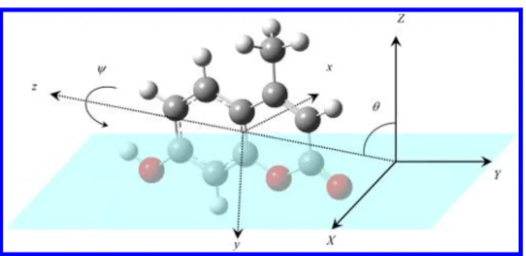
4-Methyl-7-hydroxycoumarin (MHC) and its phenoxide anion counterpart (MHC−) were chosen to demonstrate theoretical simulation of electronic SFG spectra. MHC is a pH-indicator surfactant molecule in the acidic form, while MHC−is the basic form by dissociating the phenolic proton as sketched in Figure 3a. To ﬁnd out equilibrium structures and vibrational normal modes, HF and DFT (with the B3LYP functional) calculations

Figure 3. (a) Acid−base equilibrium between 4-methyl-7-hydrox-ycoumarin (MHC, left) and its phenoxide anion (MHC−, right). (b) MHC−ﬂoating on the surface of a small water cluster, where red and dark gray spheres represent oxygen and carbon atoms, respectively.

(6)

were carried out for ground-state molecules, while CIS, CIS(D), and TD-DFT were taken for their low-lying excited states. The 6-31+G(d) basis set was applied in these calculations.

To simulate electronic SFG spectra with resonance at the sum frequency (Case 2 in section II), excitation energies for more excited states as well as transition dipole moments and polarizability-like elements between ground and resonant states were calculated (cf., eq 16). TD-DFT and CIS calculations were carried out for vertical excitation energies up to 100 states, and CIS was applied to obtain transition moments between excited states (i.e., μ⃗nm between resonant and intermediate

states). The molecular z axis was chosen parallel to the transition moment vector between ground state (g) and the resonant excited state (n), that is,μgnz ≠ 0 while μgnx =μgny = 0, to

simplify following calculations.21 All quantum chemical computations were done by using the Gaussian 09 package.26

To know the most probable orientations of the molecule when itﬂoats on the water surface, we have made a simpliﬁed DFT optimization by putting the molecule into a small water cluster (∼50 water molecules). The result, illustrated in Figure 3b, showed that oxygen atoms tend to point downward into water bulk, while the methyl group dangles outward. Although it requires molecular dynamics or other tools to clarify the overall orientation distribution, this preliminary DFT calcu-lation has given us a meaningful indication as to the tendency of molecular orientation.

IV. RESULTS AND DISCUSSION

Optimized structures of MHC/MHC− at their ground-state equilibrium wereﬁrst calculated, and vertical excitation energies and transition strengths to low-lying excited states followed. The ground states have a similar geometry, and the symmetry term is 11_A_{′ in the C}

s point group for both molecules.

Calculated excitation energies, as listed in Table 1, showed that TD-DFT gave most close values to available experimental data, while CIS and CIS(D) yielded systematic overestimation. The excitation energies of the two molecules differed notably, say, ∼1 eV for the first excited states. Despite these differences, there was one common result for both molecules with any level of calculation that thefirst excited state, 21A′, has a dominant oscillator strength, while all other low-lying states possess negligible transition strengths.

ESFG spectra with resonance at the sum frequency (Case 2 in section II) of MHC/MHC−molecules were then simulated to compare with experimental analogous results.23According to eqs 17 and 18, the ESFG proﬁles consist of two parts: transition matrix elements (μ_gni _α

ngij) and band-shape function (F).

Transition matrix elements were calculated by CIS transition

moments between all related electronic states whereω₁= 750 nm (1.65 eV) and ω₁ + ω₂ resonant with the destination excited state n. Because only the ﬁrst state (21A′) has a signiﬁcant oscillator strength upon excitation from the ground state (11_A_{′), only one n state was considered here. In principle,}

it has to include as many excited states as possible to make the hyperpolarizability converge (cf., eq 16), and in practice 100 states were taken to achieve the threshold. By the choice of molecular coordinates and symmetry, two components of transition dipole moment (μgnx andμgny) and four components of

polarizability (αngxy, etc.) vanish. The nonzero matrix elements

are listed in Table 2. It could be seen that, although the neutral molecule and its anionic counterpart have similar geometries and transition moments to theirﬁrst excited states, the overall hyperpolarizabilities came to be quite diﬀerent.

The band-shape function is composed of Franck−Condon integrals, excitation detunings, and dephasing constants. The Franck−Condon factor was evaluated by using the displace-ment-distorted harmonic oscillator as demonstrated in our previous papers,27,28and a dephasing constantΓ = 10 cm−1and an inhomogeneous broadeningσ = 500 cm−1(cf., eq 18b) were used. Combining transition matrix elements and band-shape function yielded χ_zxx(2)_, _χ

zxz

(2)_{, etc., of a single molecule. To}

correlate the orientation of this molecule to a water-surface environment in the laboratory frames,21,23 a flat distribution window of Euler angles of (θ = 80° ± 10°, ψ = 180° ± 10°) was assumed due to the tendency that oxygen atoms would point into the water (Figure 4). According to eq 26b, the SFG spectra with the sps polarization were simulated as shown in Figure 5. The calculated wavy structures came from vibronic transitions involving certain vibrational modes with large Huang−Rhys (displacement) factors.27 The profile of MHC− was broader than that of MHC, reflecting an overall larger geometric change of the former than the latter upon excitation.

Table 1. Vertical Excitation Energies (in eV, Roman Type) and Oscillator Strengths (Dimensionless, Italic Type) between the Ground State (11A′) and the Low-Lying Excited States of MHC and MHC−

MHC MHC−

state TD-DFTa CIS CIS(D) expt.b state TD-DFTa CIS CIS(D) expt.b

21_A_′ _{4.157, 0.288} _{5.184, 0.509} _4.659 _3.87 ₂1_A_′ _{3.215, 0.326} _{4.263, 0.808} _3.173 _3.44 31_A_′ _{4.499, 0.023} _{5.758, 0.003} _4.921 ₁1_A_″ _{3.368, 0.002} _{4.557, 0.010} _3.707 11_A_″ _{4.536, 0.000} _{6.312, 0.000} _5.024 ₂1_A_″ _{3.478, 0.000} _{4.943, 0.004} _4.175 41_A′ _{5.115, 0.043} _{6.673, 0.196} _6.198 ₃1_A″ _{3.935, 0.001} _{5.112, 0.008} _4.231 21_A_″ _{5.207, 0.001} _{6.400, 0.008} _5.744 ₃1_A_′ _{4.213, 0.030} _{5.213, 0.062} _4.342 51_A_′ _{5.570, 0.001} _{7.219, 0.824} _5.990 ₄1_A_″ _{4.245, 0.006} _{5.482, 0.001} _4.346

a_{With B3LYP/6-31+G(d).}b_{Estimated according to ref 25. Note that the calculations were done in the gas phase (as isolated molecule), while the}

experimental data were taken from an aqueous environment.

Table 2. Transition Matrix Elements (in atomic units) in

ESFG Resonant at the Sum Frequency of MHC and MHC−

Calculated by CIS/6-31+G(d)a MHC MHC− μgnz 1.891 2.693 αngxx 1.961 9.289 αngyy 0.030 −9.055 αngzz 0.142 −18.523 αngyz 7.659 13.189 αngzy 9.365 14.463

(7)

Although experimental SFG spectra of MHC/MHC−are not yet available, we believe that its band-shape should be similar to that of HHC/HHC− (4-heptadecyl-7-hydroxycoumarin).23 Because the electronic transition chromophore locates on the aromatic ring with little conformational change in the 4-alkyl group in both molecules, vibrational modes related to the alkyl group are supposed unaltered and therefore make little contribution to the spectral proﬁle. Eventually we could compare our simulated SFG spectra of the anion MHC−with

the experimental report of HHC−found in the basic condition from ref 23. Figure 5b shows roughly consistent spectral shapes in terms of peak positions, although the intensities of the real part have some discrepancies. The neutral species MHC and HHC, on the other hand, were expected to have a maximum at ∼320 nm, and there were no available experimental data for

comparison. Proceeding from our simpliﬁed model, the

simulated results can be further improved when considering the following factors:

(i) Non-Condon contribution. According to eq 17, non-Condon contribution such as dipole derivatives and polarizability derivatives with respect to vibrational normal coordinates were omitted for simplicity. This part could make nontrivial contribution to certain excitations especially weakly allowed and symmetry-forbidden transitions.

(ii) Molecular orientation distribution. In this preliminary simulation, only a small ﬂat distribution window of molecular orientation was assumed. To obtain more information of orientation distribution, other theoretical tools like molecular dynamics are required.

(iii) Solvent eﬀect and inhomogeneous broadening. The subtle inﬂuence of environmental solvent molecules on the excitation properties of the sample molecule was not explicitly counted in; an inhomogeneous broadening of

500 cm−1 was taken instead. This value might be

somewhat underestimate but could retain major structures in the spectral proﬁle. A larger value would be more suitable for the aqueous environment but smooth out any feature. If one wants to resolve the

extent of the solvent eﬀect, a more demanding

computation is certainly needed.

(iv) Charge effect from solute ions. In our model, the solution was assumed diluted, and each sample molecule was isolated from other solutes. Therefore, the charge effect, for example, from counterions, was not taken into account. In a real system, the existence of other ions would alter SFG intensity and spectral shape through their influence on electron density as well as on geometric structure of the sample molecule, especially when the concentration is not low. Moreover, the charged species, once condensed enough, could form an electric double layer at the surface and make the issue more complicated. It requires a larger model cluster to include other ions for an explicit computation of this effect.

(v) Spectral shape depending on computational settings. Computational level of theory and basis set affect not only excitation energies (cf., Table 1) but also geo-metrical structures, and hence influence vibronic Franck−Condon integrals involved in spectral shapes (cf., eq 17). In our spectral simulation based on DFT and CIS calculations, Huang−Rhys (displacement) factors were somehow underestimated. While peak positions were generally correct, it resulted in an overestimate on SFG intensity in the lower energy region and an underestimate in the higher energy region comparing to experimental results, for example,∼40% larger at 410 nm and ∼40% smaller at 340 nm for the amplitude of Re[χ(2)] as shown in Figure 5b. A similar trend could be seen in the amplitude of Im[χ(2)], although it was not as Figure 4.Definitions of laboratory frames (XYZ, with Z defined along

surface normal), molecular coordinates (xyz), and Euler angles (tilt angle θ and twist angle ψ) of MHC ﬂoating on the (averaged, ﬂattened) water surface.

Figure 5.Simulated ESFG spectra of (a) MHC and (b) MHC−with the sps polarization. The experimental data of HHC−from ref 23 were drawn in (b) for comparison.

(8)

obvious. A higher level calculation is expected to improve the overall result.

Should these factors be included or corrected, a reﬁned picture would be obtained. This approach is going to be applied onto the larger molecule HHC/HHC− as well, which is our next step to make a more compact combination of experimental and theoretical studies.

V. SUMMARY

In this work, we have presented general mathematical formulas of electronic sum-frequency generation spectroscopy and discussed cases under particular resonant conditions. By ﬁrst-principle calculations, we could obtain necessary elements such as geometric structures, excitation energies, transition dipole moments, hyperpolarizabilities, etc., of a molecule for the theoretical simulation of its ESFG spectra. To demonstrate the capability of this formulation, we have taken 4-methyl-7-hydroxycoumarin and its anionic counterpart as an example and illustrated the spectra for a single molecule at a speciﬁc orientation distribution. For more detailed comparison with or for more accurate prediction to experimental results, one could further introduce other theoretical tools such as molecular dynamics to provide information such as the overall orientation distribution. It turns out our theoretical approach could complement experimental SFG technique in exploring the sciences of surfaces and interfaces.

■

AUTHOR INFORMATION

Corresponding Author

*E-mail: [email protected].

Notes

The authors declare no competingﬁnancial interest.

■

ACKNOWLEDGMENTS

This research was supported by a grant from the National Science Council (Grant No. 102-2113-M-002-011) of Taiwan, ROC.

■

REFERENCES

(1) Shen, Y. R. The Principles of Nonlinear Optics; John Wiley & Sons: New York, 1984.

(2) Lin, S. H.; Hayashi, M.; Islampour, R.; Yu, J.; Yang, D. Y.; Wu, G. Y. C. Molecular Theory of Second-Order Sum-Frequency Generation. Physica B 1996, 222, 191−208.

(3) Hayashi, M.; Lin, S. H. Molecular Theory of Sum-Frequency Generations and Its Applications to Study Molecular Chirality. In Advances in Multi-photon Processes and Spectroscopy; Lin, S. H., Villaeys, A. A., Fujimura, Y., Eds.; World Scientiﬁc: Singapore, 2004; Vol. 16, pp 307−422.

(4) Wei, X.; Hong, S.-C.; Lvovsky, A. I.; Held, H.; Shen, Y. R. Evaluation of Surface vs Bulk Contributions in Sum-Frequency Vibrational Spectroscopy Using Reflection and Transmission Geo-metries. J. Phys. Chem. B 2000, 104, 3349−3354.

(5) Wei, X.; Miranda, P. B.; Zhang, C.; Shen, Y. R. Sum-Frequency Spectroscopic Studies of Ice Interfaces. Phys. Rev. B 2002, 66, 085401. (6) Du, Q.; Superfine, R.; Freysz, E.; Shen, Y. R. Vibrational Spectroscopy of Water at the Vapor/Water Interface. Phys. Rev. Lett. 1993, 70, 2313−2316.

(7) Ostroverkhov, V.; Waychunas, G. A.; Shen, Y. R. New Information on Water Interfacial Structure Revealed by Phase-Sensitive Surface Spectroscopy. Phys. Rev. Lett. 2005, 94, 046102.

(8) Shen, Y. R.; Ostroverkhov, V. Sum-Frequency Vibrational Spectroscopy on Water Interfaces: Polar Orientation of Water Molecules at Interfaces. Chem. Rev. 2006, 106, 1140−1154.

(9) Ji, N.; Ostroverkhov, V.; Tian, C. S.; Shen, Y. R. Characterization of Vibrational Resonances of Water−Vapor Interfaces by Phase-Sensitive Sum-Frequency Spectroscopy. Phys. Rev. Lett. 2008, 100, 096102.

(10) Tian, C.-S.; Shen, Y. R. Isotopic Dilution Study of the Water/ Vapor Interface by Phase-Sensitive Sum-Frequency Vibrational Spectroscopy. J. Am. Chem. Soc. 2009, 131, 2790−2791.

(11) Tian, C. S.; Shen, Y. R. Sum-Frequency Vibrational Spectroscopic Studies of Water/Vapor Interfaces. Chem. Phys. Lett. 2009, 470, 1−6.

(12) Zhuang, X.; Miranda, P. B.; Kim, D.; Shen, Y. R. Mapping Molecular Orientation and Conformation at Interfaces by Surface Nonlinear Optics. Phys. Rev. B 1999, 59, 12632−12640.

(13) Gautam, K. S.; Schwab, A. D.; Dhinojwala, A.; Zhang, D.; Dougal, S. M.; Yeganeh, M. S. Molecular Structure of Polystyrene at Air/Polymer and Solid/Polymer Interfaces. Phys. Rev. Lett. 2000, 85, 3854−3857.

(14) Chen, C.; Wang, J.; Woodcock, S. E.; Chen, Z. Surface Morphology and Molecular Chemical Structure of Poly(n-butyl methacrylate)/Polystyrene Blend Studied by Atomic Force Micros-copy (AFM) and Sum-Frequency Generation (SFG) Vibrational Spectroscopy. Langmuir 2002, 18, 1302−1309.

(15) Hayashi, M.; Lin, S. H.; Raschke, M. B.; Shen, Y. R. A Molecular Theory for Doubly Resonant IR−UV-Vis Sum-Frequency Generation. J. Phys. Chem. A 2002, 106, 2271−2282.

(16) Moad, A. J.; Simpson, G. J. A Unified Treatment of Selection Rules and Symmetry Relations for Sum-Frequency and Second Harmonic Spectroscopies. J. Phys. Chem. B 2004, 108, 3548−3562.

(17) Lin, C.-K.; Shih, C.-C.; Niu, Y.; Tsai, M.-Y.; Shiu, Y.-J.; Zhu, C.; Hayashi, M.; Lin, S. H. Theoretical Study on Structure and Sum-Frequency Generation (SFG) Spectroscopy of Styrene−Graphene Adsorption System. J. Phys. Chem. C 2013, 117, 1754−1760.

(18) Yamaguchi, S.; Tahara, T. Precise Electronic χ(2) _{Spectra of}

Molecules Adsorbed at an Interface Measured by Multiplex Sum Frequency Generation. J. Phys. Chem. B 2004, 108, 19079−19082.

(19) Yamaguchi, S.; Tahara, T. Heterodyne-Detected Electronic Sum Frequency Generation:‘Up’ versus ‘Down’ Alignment of Interfacial Molecules. J. Chem. Phys. 2008, 129, 101102.

(20) Mondal, S. K.; Yamaguchi, S.; Tahara, T. Molecules at the Air/ Water Interface Experience a More Inhomogeneous Solvation Environment than in Bulk Solvents: A Quantitative Band Shape Analysis of Interfacial Electronic Spectra Obtained by HD-ESFG. J. Phys. Chem. C 2011, 115, 3083−3089.

(21) Watanabe, H.; Yamaguchi, S.; Sen, S.; Morita, A.; Tahara, T. ‘Half-Hydration’ at the Air/Water Interface Revealed by Heterodyne-Detected Electronic Sum Frequency Generation Spectroscopy, Polarization Second Harmonic Generation, and Molecular Dynamics Simulation. J. Chem. Phys. 2010, 132, 144701.

(22) Yamaguchi, S.; Bhattacharyya, K.; Tahara, T. Acid−Base Equilibrium at an Aqueous Interface: pH Spectrometry by Heterodyne-Detected electronic Sum Frequency Generation. J. Phys. Chem. C 2011, 115, 4168−4173.

(23) Yamaguchi, S.; Kundu, A.; Sen, P.; Tahara, T. Communication: Quantitative Estimate of the Water Surface pH Using Heterodyne-Detected Electronic Sum Frequency Generation. J. Chem. Phys. 2012, 137, 151101.

(24) Drummond, C. J.; Warr, G. G.; Grieser, F.; Ninham, B. W.; Evans, D. F. Surface Properties and Micellar Interfacial Microenviron-ment of n-Dodecylβ-D-Maltose. J. Phys. Chem. 1985, 89, 2103−2109. (25) Drummond, C. J.; Grieser, F. Absorption Spectra and Acid− Base Dissociation of the 4-Alkyl Derivatives of 7-Hydroxycoumarin in Self-Assembled Surfactant Solution: Comments on Their Use as Electrostatic Surface Potential Probes. Photochem. Photobiol. 1987, 45, 19−34.

(26) Frisch, M. J.; Trucks, G. W.; Schlegel, H. B.; Scuseria, G. E.; Robb, M. A.; Cheeseman, J. R.; Scalmani, G.; Barone, V.; Mennucci, B.; Petersson, G. A.; et al. Gaussian 09, revision A.02; Gaussian, Inc.: Wallingford, CT, 2009.

(9)

(27) Lin, C.-K.; Li, M.-C.; Yamaki, M.; Hayashi, M.; Lin, S. H. A Theoretical Study on the Spectroscopy and the Radiative and Non-Radiative Relaxation Rate Constants of the S0 1A1 ― S1 1A2

Vibronic Transitions of Formaldehyde. Phys. Chem. Chem. Phys. 2010, 12, 11432−11444.

(28) Li, J.; Lin, C.-K.; Li, X. Y.; Zhu, C. Y.; Lin, S. H. Symmetry Forbidden Vibronic Spectra and Internal Conversion in Benzene. Phys. Chem. Chem. Phys. 2010, 12, 14967−14976.