國立交通大學
應用數學系
碩 士 論 文
三維封閉曲面上的圖形切割線
Cut Graph of Three Dimensional Closed Surfaces
研 究 生:蔣卓時
指導教授:張書銘 博士
三維封閉曲面上的圖型切割線
Cut Graph of Three Dimensional Closed Surfaces
研 究 生:蔣卓時
指導教授:張書銘 博士
Student: Juo-Shir Chung
Advisor: Dr. Shu-Ming Chang
國 立 交 通 大 學
應 用 數 學 系
碩 士 論 文
A Thesis
Submitted to Department of Applied Mathematics
College of Science
National Chiao Tung University
in Partial Fulfillment of the Requirements
for the Degree of
Master
in
Applied Mathematices
June 2012
Hsinchu, Taiwan, Republic of China
三維封閉曲面上的圖形切割線
學生:蔣卓時
指導教授:張書銘
博士
國立交通大學應用數學系(研究所)碩士班
摘
要
一個在三維空間的封閉曲面,使用三角網格將其離散化,搭配半邊結構的方式將其儲存在 電腦中。本論文將對三種不同類型的封閉曲面 (球,虧格數1,虧格數1接合虧格數1) 進 行探討,欲將該封閉曲面進行切割,使得其沿著圖形切割線能將曲面展開成不同型態的基 本定義域 (fundamental domain),進而創建覆蓋空間 (covering space)。在實作三維封閉曲 面上的圖形切割線時,運用兩種不同的演算法分別在不同的的權重 (weight) 下,控制生成 的圖形切割線。不同的演算法分別在不同的權重下,分別得出了不同的圖形切割線,但是 每一條圖形切割線的走勢並不完全依照當初設計權重的希望進行。Cut Graph of Three Dimensional Closed Surfaces
Student: Juo-Shir Chung
Advisors: Dr. Shu-Ming Chang
Department (Institute) of Applied Mathematics
National Chiao Tung University
Abstract
A closed surface in three-dimensional space, using the triangular meshes to discrete, with half edge structure will be stored in the computer. This work will have three different types of closed surface (ball, genus of one, genus of two) to discuss, For the closed surface to cut, cutting down the cut graph able to transform surfaces into different types of fundamental domain, and thus created covering space. Working cut graph on closed surface of the three-dimensional using two different algorithms with different weights to control generated cut graph. Different algorithms with different weights, get different cut graph, but cut graph does not completely in accordance with the original design weight hope.
Contents
1 Introduction 1
1.1 related work . . . 1
2 Model and Theory 2 2.1 ball, genus of one, and genus of two . . . 2
2.2 triangular meshes . . . 4
2.2.1 half-edge data structure . . . 5
2.3 cut graph . . . 6
2.4 fundamental domain . . . 7
2.5 universal covering space . . . 7
2.6 minimum spanning tree . . . 8
3 Algorithms 8 3.1 half edge database . . . 8
3.2 dual mesh . . . 9
3.3 minimum spanning tree . . . 9
3.4 cut graph and further improved by pruning the branches . . . 12
3.5 cut graph element . . . 12
4 Numerical Simulations 13 4.1 dual mesh in ball, genus of one, and genus of two . . . 13
4.2 minimum spanning tree in three models . . . 17
4.3 cut graph and pruning the branches in three models . . . 29
4.4 prune the branch . . . 35
4.5 compare two kinds of minimal spanning tree algorithms . . . 36
4.6 affect of the weight with minimal spanning tree . . . 39
5 Conclusion and Future Work 42
List of Figures
1 ball . . . 2 2 genus of one . . . 3 3 genus of two . . . 4 4 Kruskal algorithm . . . 10 5 Prim algorithm . . . 126 ball dual mesh . . . 13
7 ball dual mesh project to xy plane . . . . 14
8 genus of one dual mesh . . . 14
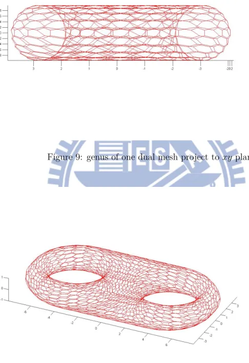
9 genus of one dual mesh project to xy plane . . . . 15
10 genus of two dual mesh . . . 15
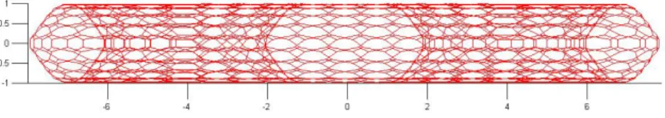
11 genus of two dual mesh project to xy plane . . . . 16
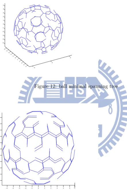
12 ball minimal spanning tree . . . 17
13 ball minimal spanning tree project to xy plane . . . . 17
14 ball minimal spanning tree project to yz plane . . . . 18
15 ball minimal spanning tree project to xz plane . . . . 18
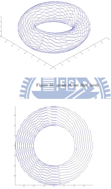
16 genus of one dual mesh . . . 19
17 genus of one dual mesh project to xy plane . . . . 19
18 genus of one dual mesh project to yz plane . . . . 20
19 genus of one dual mesh project to xz plane . . . . 20
20 genus of two dual mesh . . . 21
21 genus of two dual mesh project to xy plane . . . . 21
22 genus of two dual mesh project to yz plane . . . . 22
23 genus of two dual mesh project to xz plane . . . . 22
24 ball minimal spanning tree with change starting point . . . 23
25 ball minimal spanning tree project to xy plane with change starting point . . . 23
26 ball minimal spanning tree project to yz plane with change starting point . . . 24
27 ball minimal spanning tree project to xz plane with change starting point . . . 24
28 genus of one minimal spanning tree with change starting point . . . 25
29 genus of one minimal spanning tree project to xy plane with change starting point . . . 25
30 genus of one minimal spanning tree project to yz plane with change starting
point . . . 26
31 genus of one minimal spanning tree project to xz plane with change starting point . . . 26
32 genus of two minimal spanning tree with change starting point . . . 27
33 genus of two minimal spanning tree project to xy plane with change starting point . . . 27
34 genus of two minimal spanning tree project to yz plane with change starting point . . . 28
35 genus of two minimal spanning tree project to xz plane with change starting point . . . 28
36 Ball cut graph . . . 29
37 Ball cut graph project to xz plane . . . . 29
38 Ball cut graph project to yz plane . . . . 30
39 Ball cut graph project to xy plane . . . . 30
40 genus of one cut graph . . . 31
41 genus of one cut graph project to xz plane . . . . 31
42 genus of one cut graph project to yz plane . . . . 32
43 genus of one cut graph project to xy plane . . . . 32
44 genus of two cut graph . . . 33
45 genus of two cut graph project to xz plane . . . . 33
46 genus of two cut graph project to yz plane . . . . 34
47 genus of two cut graph project to xy plane . . . . 34
48 ball cut graph with pune . . . 35
49 genus of one cut graph with pune . . . 35
50 genus of two cut graph with pune . . . 36
51 genus of two cut graph Prim and Kruskal algorithm . . . 37
52 genus of two cut graph Prim with Kruskal algorithm . . . 37
53 genus of two cut graph Prim and Kruskal algorithm . . . 38
54 genus of two cut graph Prim and Kruskal algorithm . . . 38
55 genus of one cut graph weight with distance . . . 39
56 genus of two cut graph weight with distance . . . 40
1
Introduction
Growing three-dimensional image processing technology in recent years, three-dimensional images is greatly increased demand technology, a wide range of three-dimensional technol-ogy application, for example, when doctors determine the patient’s condition, the three-dimensional image was even more important than the traditional image effect, allows doctors to judge the condition is more favorable, but also more and less error-prone.
The rise in recent years, three-dimensional images, the vast majority are with the Depart-ment of Information Engineering, the use of computer technology with a variety of algorithms in the re-construction of a three-dimensional computer model, these things sound with the Department of Mathematics and little relevance, but in fact chase the final analysis the origin of mathematics from the geometry of the concept of law exhibited, which explains why the geometry will learn the discipline of the Department of Mathematics at the rear section, De-partment of Mathematics repair all disciplines are in order to get to the bottom of geometric science, while the various disciplines of specialization are also developed from the geometric problems.
The to great geometer usually are great mathematician For Science and Technology, De-partment of Mathematics of the geometry of three-dimensional images in fact should be a greater output, Shing-Tung Yau teacher will utilize the operator of the the topology geome-try of conformal more details on modeling three-dimensional graphics can be retained more complete three-dimensional model.
This work introduces the theory, algorithm and mathematical tools, creat surface by Mefisto then realize the cut graph.
1.1
related work
Xiaotian Yin, Miao Jin, Xianfeng Gu teacher in Computing Shortest Cycles Using Uni-versal Covering Space[9], the three-dimensional image into a two-dimensional fundamental domain and use of the concept of covering space topology to find the shortest Shortest Cy-cles[10] after Wei Hong Xianfeng Gu Feng Qiu Miao Jin Arie Kaufman teachers in conformal the Virtual colon Flattening the use of the concept of conformal inside the human colon fundamental domian into two-dimensional and retained many of the details from the three-dimensional impact[6].
domain must be working-Cut Graph.
2
Model and Theory
All model in this work are created by Mefisto[2][1].
2.1
ball, genus of one, and genus of two
Genus
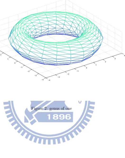
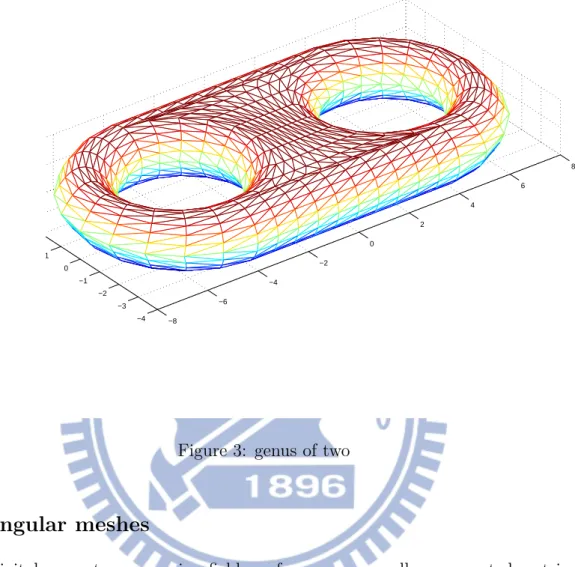
We define the genus of an orientalie surface to be the number of handles we add to the sphere to get the surface,it is topological invariant[3].
−10 −5 0 5 10 −10 −5 0 5 10 −6 −4 −2 0 2 4 6 Figure 1: ball
−4 −3 −2 −1 0 1 2 3 4 −4 −3 −2 −1 0 1 2
−8 −6 −4 −2 0 2 4 6 8 −4 −3 −2 −1 0 1
Figure 3: genus of two
2.2
triangular meshes
In the digital geometry processing field, surfaces are generally represented as triangular meshes, which are directly supported by common graphicss hardware. Any other geometric representations, such as splines, implicit surfaces, and level sets, need to be converted to triangular meshes for display purposes.
The popularity of triangular meshes can be explained in term of both theory and practice. In theory, any surface with C1 continuity can be triangulated. Simplicial homology and
simplicial cohomology theories in topology are directly based on the triangular meshes. All surfaces in real life can be digitized using 3D scanners. The acquired point clouds can be easily converted to triangulated meshs. Most digital geometry processing softwares support trigular meshes as the default internal data structure. More importantly,modern graphics hardware supports triangular meshes directly.
A triangular mesh is exactly a two-dimensional simplicial complex in algebraic topology. Intuitively, a mesh is a set of triangular faces coherently. Glued together.All of the topological
information is implied by the connectivity. In general, a mesh is embedded in R3. A mesh is
flat everywhere except at the vertices, where the curvatures can be defined and measured. Topological problems can be solve accurately on meshes without any approximation. Dif-ferential forms, curvatures, geodesics, and conformal mappings can only be solved on meshes by approximation[4].
2.2.1 half-edge data structure
A half-edge data structure is commonly used in geometric softwares to represrnt triangular meshes.
A mesh M = (V, E, F ) consists of a list of vertices V, edge E, and face F. Suppose
V = {v0, v1, ..., vn} is the list of vertices of a mesh M. In the following discussion, we use
{v1, v2, ..., vk} to represent the set of vertices and [v1, v2, ..., vk] the set of ordered vertices. For
example, {vi, vj} represents a non-orientied edge connecting vi and vj; [vi, vj] represents an
oriented edge, starting from vi and ending at vj. We call an oriented edge a half-edge, denote
as hij =[vi,vj] where vi is called the source the vertex and vjis the target vertex.
Suppose three vertices {vi, vj, vk} from a face, then all the permutations of vi, vj, vk can
be divided into two classes. If two permutations differ by an even number of swaps, then the two permutations are equivalent; if two permutations differ by odd number of swaps, then they are not equivalent.
Definition 2.1 (Face Orientation). Each equivalence class of the permutation of the vertices
define one orientation of the face.
This mean, the orientation of [vi, vj, vk] and [vj, vk, vi]are the same; the orientation of [vi,
vj, vk] and [vj, vi, vk] are opposite.
Definition 2.2 (Boundary). The boundary of an oriented face [vi, vj, vk] is
∂[vi, vj, vk] = [vi, vj] + [vj, vk] + [vk, vi].
The boundary of an oriented edge [vi, vj] is
∂[vi, vj] = vi− vj.
Each edge eij ={vi, vj} has two orientations, hij = [vi, vj] and hji = [vj, vi]. We say the
half-edge are dual to each other.
Definition 2.3 (Dual Half-Edge). Suppose an oriented edge is hij = [vi, vj]. We call half-edge
Definition 2.4 (Interior Edge). Suppose an edge in the mesh attaches to two faces, then the
edge is called an interior edge. The half-edges attached to it are called interior half-edges.
Definition 2.5 (Boundary Edge). Suppose an edge in the mesh attaches to only one face, then
the edge is called a boundary edge. The half-edges attach to it is called boundary half-edges.
Each face {vi, vj, vk} has two otientations [vi, vj, vk] and [vj, vi, vk]. Each orientation gives
a set of boundary half-egdes: [vi, vj, vk] gives { [vi, vj], [vj, vk], [vj, vk]}; [vj, vi, vk] gives {
[vj, vi], [vk, vj], [vi, vk]}. Suppise we choose an orientation for each face, then we define the
half-edge set of the mesh union of the boundary half-edges of all the oriented faces. We use
F to represent the set of all oriented faces, H(M ) = ∪
[vi,vj,vk]∈F
∂[vi, vj, vk].
If we can choose the orientations of all faces in a consistent way, such that any interior edge attaches to a pair of dual half-edges in H(M ), then the mesh is orientable.
Definition 2.6 (Mesh Orientation). Given a mesh M , if one can choose the orientation of
each face, the oriented face set id F, then for ant interior edge eij ={vi, vj}, [vi, vj] and [vj, vi]
are in H(M ), then M is orientable.
2.3
cut graph
A cut graph on a mesh is a set of edges, such that its complement is a topological disk, which includes all the faces. All the topological information of the mesh is encoded in the cut graph.
Definition 2.7 (Cut Graph). A cut graph G in a mesh M consists of a set of edges of M ,
such that M /G is a simply connected mesh.
A simply connected mesh has no handle and only one boundary, namely, it is a topological disk. In order to compute the topology of the mesh, we need to compute the cut graph.
Frist, we construct a dual mesh of M . A dual mesh ¯M is the mesh constructed in the
fllowing way:
1. Each face f in M corresponds to a unique vertex of ¯v(f ) ∈ ¯M .
Suppose the faces adjacent to v are f1, f2, ..., fn ∈ Msorted counter-clock-wisely. Then
¯
f (v) = [¯v(f1), ¯v(f2), ..., ¯v(fn)].
3.Each edge e ∈ Madjacent to faces fi, f j∈ M corresponds to an edge e,
¯
e = [¯v(fi), ¯v(fj)]. Algorithm 1 Cut Graph.
Require: A mesh M
Ensure: A cut graph G of M ;
1: Compute the dual mesh ¯M of M ;
2: Generate a minimal spanning tree ¯T of the vertices of ¯M ;
3: G={ e | ¯e /∈ ¯T };
4: return G;
The idea of the algorithm is to remove a topological disk D from M . D is as big as possible, such that by removing D, only a one-dimensional graph consisting of vertices and edges is left. Therefore, the cut graph G equals to M /D. A spanning tree of vertices of ¯M
corresponds to a topological disk consisting of all faces of M .
The cut graph is not unique, it depends on the construct of the minimal spanning tree ¯T .
The spamming tree could be generated using DFS(depth first search) or BFS(breadth first search), it also depends on the chosen root vertex.
The cut graph can be further improved by pruning the branches[5].
2.4
fundamental domain
The fundamental domain of a mesh is a topological disk which consists of all faces of M . Fundamental domain is important for many applications, such as surface parameterization and surface matching.
2.5
universal covering space
the construction of a finite portion of the universal covering space is to coherently glue copies of the fundamental domains. The most difficult part is to guarantee the consistency.
Given a closed mesh M , first we compute a cut graph G. Then we locate all of the branching vertices in G, which separate the cut graph into segments. Each segment is as-signed an orientation, which is arbitrarily chosen. All of the oriented segments are denotes
as{s1, s2, ..., sn}. We slice the mesh M along the cut graph G to get the fundamental domain
of M , denoted as D. The boundary of D consists of oriented segments,
∂D = sd1 i1s d2 i2...s dm im where ik∈ 1, 2, ..., n, dk∈ +1, −1, 1 ≤ k ≤ m.
We denote the finite portion of the universal covering space of M as ¯M . We initialize the
¯
M as one copy of the fundamental domain D. Then we merge a new copy of D with the
current ¯M in the following way. Suppose an oriented segment s+1k is on the boundary of ¯M , s−1k ∈ ∂ ¯M , then s−1k is on the boundary of D. We merge D with ¯M by gluing s−1k to s+1
k ,
denote as
¯
M = ¯M ∪skD.
Suppose the boundary of the new ¯M is
∂ ¯M = sd1 i1s d2 i2...s dn in.
Find a consecutive pair of segment sdk ik,s
dk+1
ik+1, such that ik = ik+1,dk =−dk+1, namely
(sdk
ik)−1 = s dk+1 ik+1.
Then stitch the boundary along sdk ik ans s
dk+1
ik+1. We repeat this stitching process, until there is
no such consecutive opposite pairs of segments in the boundary of ¯M .
We can repeat this process to glue more copies of the fundamental domain to enlarge the universal covering space unsil it is big enough for our purpose[5].
2.6
minimum spanning tree
Definition 2.8 (Spanning Tree). That graph is a subgraph that is a tree and connects all the
vertices together.
Definition 2.9 (Minimum Spanning Tree). A spanning tree with weight less than or equal to
the weight of every other spanning tree.
3
Algorithms
3.1
half edge database
Algorithm 2 half edge
1: array half edge;
2: for (each edge of element,from Pi to Pj) do
3: hij = 1;
4: end for
3.2
dual mesh
We make a point represent a face(element), this point don’t have relationship with face, and we a face represent a interior point, if for each face(element) has connect face(element) then we connect the point with dual edge in the dual space, boundary edge and boundary point will be vanish in the dual space, that mean we will not affact the boundary.
Note:In this work we use the Center of gravity.
Algorithm 3 Dual edge
1: array dual edge;
2: for (each element) do
3: if(element i is conncet to element j)
4: dij = 1;
5: end for
6: for (each dual edge) do
7: connect each edge;
8: end for
3.3
minimum spanning tree
Weight
We give the cost for edge, weight can affect the Minimal spanning tree, so we choose weight for what you went to get[7].
1.If you went your cut graph can be short, you can let weight=half edge length
2.If you went your cut graph can be smooth, you can let weight=conner of two elements.
Part A.Kruskal
This algorithm is known as a greedy algorithm.
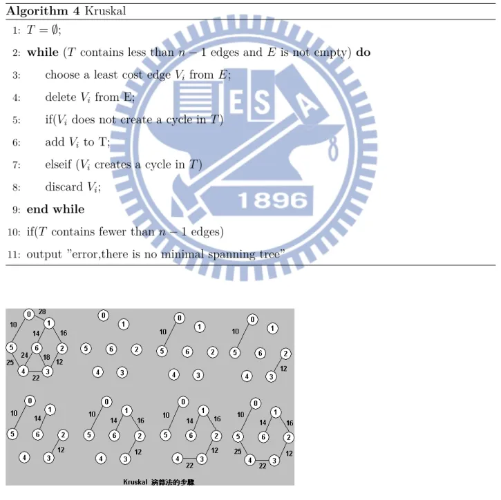
Build a minimum cost spanning tree T by adding edges to T one at a time. Select the edges for inclusion in T in increaseing order of their weight. An edge is added to T if it does not form a cycle with the edges that are already in T . Exactly n− 1 edges will be selected for inclusion in T .
Note: that, whenever you add an edge (u, v), it’s always the smallest connecting the part of
S reachable from u with the rest of G, so by the lemma it must be part of the MST.
Algorithm 4 Kruskal
1: T = ∅;
2: while (T contains less than n− 1 edges and E is not empty) do
3: choose a least cost edge Vi from E;
4: delete Vi from E;
5: if(Vi does not create a cycle in T )
6: add Vi to T;
7: elseif (Vi creates a cycle in T )
8: discard Vi;
9: end while
10: if(T contains fewer than n− 1 edges)
11: output ”error,there is no minimal spanning tree”
Figure 4: Kruskal algorithm
Prim’s algorithm, like Kruskal’s, constructs the minimum-cost spanning tree one edge at a time.
The main difference:
1.The set of selected edges forms a tree at all times in Prim’s algorithm. 2.The set of selected edges in Kruskal’s algorithm forms a forest at each stage.
Prim’s algorithm begins with a tree, T , that contains an arbitrary single vertex. Next, we add a least cost edge (u, v) to T such that T ∪ (u, v) is also a tree. We repeat this edge addition until T contains n− 1 edges[8].
Since each edge added is the smallest connecting T to G− T , the lemma we proved shows that we only add edges that should be part of the MST. It looks like the loop has a slow step in it. But again, some data structures can be used to speed this up.
Algorithm 5 Prim
1: T = ∅;
2: T V ={0};
3: while (T contains fewer than n− 1 edges) do
4: let (u, v) be a least cost edge such that u ∈ T V and v /∈ T V ; 5: if(there is no such edge)
6: break;
7: add v to T V ;
8: add (u, v) to T ;
9: end while
10: if(T contains fewer than n− 1 edges)
11: output ”error,there is no minimal spanning tree”
Note:If the vertex of the edge is in the minimal spanning tree then we pick next minimum
weight edge.
Part C.Sollin
Although rediscovered by Sollin in the 1960’s.
Sollin’s algorithm selects several edges for inclusion in T at each stage At the start of a stage, the selected edges, together with all the n vertices, form a spanning forest During a
Figure 5: Prim algorithm
stage, we select one edge for each tree in the forest.
This edge is a minimum cost edge that has exactly one vertex in the tree. Since two trees in the forest could select the same edge, we need to eliminate multiple copies of edges. At the start of the first stage the set of selected edges is empty. The algorithm terminates when there is only one tree at the end of a stage or no edges remain for selection.
3.4
cut graph and further improved by pruning the branches
So we delete the Minimal spanning tree last edge is Cut Graph in the dual space, we needs recover to 3-D space, We can transform dual edge and half edge by dual edge and half edge relationship, but we just need loops of Cut Graph, so we prune.
Note:Cut graph is connected component, and it’s gluing by loops after
pruning.
Algorithm 6 Prune the cut graph
1: A cut graph G of M ;
2: while there is valence one node v in G′ do
3: remove v and the segment attached to it 4: end while
5: return G′
3.5
cut graph element
Algorithm 7 re-create the element
1: A cut graph G of M ;
2: for number of the element do
3: vertex of the cut graph vi+1, vi+2, ..., vi+n where i is umber of the cut graph, n is
number of vertex of the cut graph
4: if the edge of two element, and the edge is cut graph, change one of the element
5: end for
4
Numerical Simulations
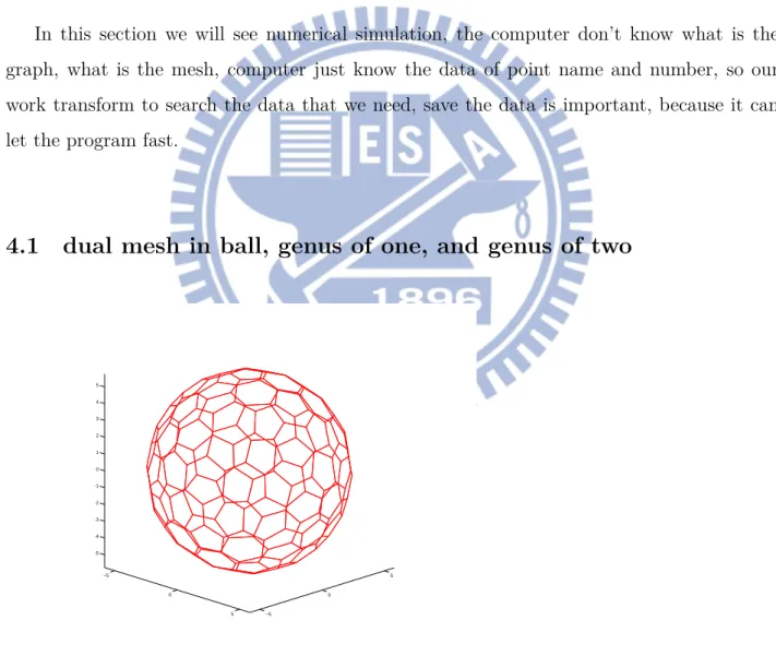
In this section we will see numerical simulation, the computer don’t know what is the graph, what is the mesh, computer just know the data of point name and number, so our work transform to search the data that we need, save the data is important, because it can let the program fast.
4.1
dual mesh in ball, genus of one, and genus of two
−5 0 5 −5 0 5 −5 −4 −3 −2 −1 0 1 2 3 4 5
−5 −4 −3 −2 −1 0 1 2 3 4 5 −50 5 −5 −4 −3 −2 −1 0 1 2 3 4 5
Figure 7: ball dual mesh project to xy plane
Figure 9: genus of one dual mesh project to xy plane
Figure 11: genus of two dual mesh project to xy plane
We can see the triangular mesh transform to dual mesh. Points of the dual mesh is a triangular mesh, face of the dual mesh is an initerior point of triangular mesh, shape of the face is not fixed, because every line that connect any two point represent ant two triangular mesh that are connect or not.
4.2
minimum spanning tree in three models
−5 −4 −3 −2 −1 0 1 2 3 4 5 −5 0 5 −5 −4 −3 −2 −1 0 1 2 3 4 5Figure 12: ball minimal spanning tree
−5 −4 −3 −2 −1 0 1 2 3 4 5 −50 5 −5 −4 −3 −2 −1 0 1 2 3 4 5
−50 5 −5 −4 −3 −2 −1 0 1 2 3 4 5 −5 −4 −3 −2 −1 0 1 2 3 4 5
Figure 14: ball minimal spanning tree project to yz plane
−5 −4 −3 −2 −1 0 1 2 3 4 5 −50 5 −5 −4 −3 −2 −1 0 1 2 3 4 5
Figure 16: genus of one dual mesh
Figure 18: genus of one dual mesh project to yz plane
Figure 20: genus of two dual mesh
Figure 22: genus of two dual mesh project to yz plane
Figure 23: genus of two dual mesh project to xz plane
The minimum spanning tree is done in the dual mesh, we create dual mesh to gain connect surface, if we do minimum spanning tree in the triangular mesh, it’s possible cutting off the surface.
The minimum spanning tree is unique or not depends on the weight, if weight is the same of every branch then the minimum spanning tree is not unique, because which branch will be gain in Kruskal algorithm or which point is the begin point in Prim algorithm.
Use the Mefisto create the triangular mesh is regular, and we use center of gravity to create dual mesh, it’s make some weight of branch are the same, so the minimum spanning tree is the unique.
We change starting point of the Prim algorithm with original starting point of the Prim al-gorithm. −5 −4 −3 −2 −1 0 1 2 3 4 5 −5 0 5 −5 −4 −3 −2 −1 0 1 2 3 4 5
Figure 24: ball minimal spanning tree with change starting point
−5 −4 −3 −2 −1 0 1 2 3 4 5 −50 5 −5 −4 −3 −2 −1 0 1 2 3 4 5
Figure 26: ball minimal spanning tree project to yz plane with change starting point −5 −4 −3 −2 −1 0 1 2 3 4 5 −50 5 −5 −4 −3 −2 −1 0 1 2 3 4 5
Figure 28: genus of one minimal spanning tree with change starting point
Figure 30: genus of one minimal spanning tree project to yz plane with change starting point
Figure 32: genus of two minimal spanning tree with change starting point
Figure 34: genus of two minimal spanning tree project to yz plane with change starting point
Figure 35: genus of two minimal spanning tree project to xz plane with change starting point
It is the same, in next subsection we will compare cut graph with change starting point Prim algorithm and Kruskal algorithm.
4.3
cut graph and pruning the branches in three models
−5 0 5 −5 0 5 −6 −4 −2 0 2 4 6Figure 36: Ball cut graph
−5 −4 −3 −2 −1 0 1 2 3 4 5 −6 −4 −2 0 2 4 6
−5 −4 −3 −2 −1 0 1 2 3 4 5 −6 −4 −2 0 2 4 6
Figure 38: Ball cut graph project to yz plane
−5 −4 −3 −2 −1 0 1 2 3 4 5 −5 −4 −3 −2 −1 0 1 2 3 4 5
Figure 40: genus of one cut graph
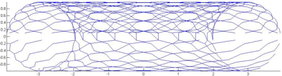
Figure 42: genus of one cut graph project to yz plane
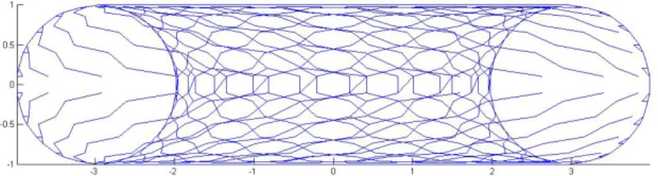
Figure 44: genus of two cut graph
Figure 46: genus of two cut graph project to yz plane
4.4
prune the branch
Figure 48: ball cut graph with pune
Figure 50: genus of two cut graph with pune
4.5
compare two kinds of minimal spanning tree algorithms
Minimal spanning tree is not unique, so cut graph is not unique, we compare two algo-rithm.
Two algorithm find the same minimal spanning tree, because Kruskal algorithm first step is sort accord to weight, Prim first have to pick first point, so these reason can make two algorithm get the same cut graph.
Figure 51: genus of two cut graph Prim and Kruskal algorithm
Figure 52: genus of two cut graph Prim with Kruskal algorithm
Figure 53: genus of two cut graph Prim and Kruskal algorithm
Figure 54: genus of two cut graph Prim and Kruskal algorithm
4.6
affect of the weight with minimal spanning tree
We try to control cut graph, we have many requirement in all case, like sometimes we need cutgraph can be short or cut graph through the conner of two mesh is the smallest.
Distance
Algorithm 8 distance
1: a dual edge ¯eij
2: eij is correspond edge of the mesh
3: length of eij
Figure 56: genus of two cut graph weight with distance
conner
Algorithm 9 conner
1: a dual edge ¯eij, where ¯vi, ¯vi are two vertex of the ¯eij
2: fi,fj are face correspond the ¯vi, ¯vi
3: ni,ni are normal vector of fi,fj
Figure 57: genus of two cut graph weight with conner
5
Conclusion and Future Work
Cut graph is tool for search handle loop and tunnel loop, but if cut graph can be smooth, the boundary of fundamental domain can be well.
We try to control the cut graph with the weight, but we can not control completely.
It means if we went to control cut graph, we have to change the algorithm of the minimal spanning tree.
Future work
We can make the algorithm speed up, dual mesh is important in this idea, but we don’t compute dual mesh, just make the number of element consist, and tell the computer every triangular mesh is connect to who, the number of two connect triangular mesh will be edge in the dual mesh, we just use half edge data then we can do next work.
Use the cut graph can create covering space, now we have cut graph, cut graph is consist by some loops, each loop is edge of fundamental domain, then copy fundamental domain and connect corresponding to the edge.
Appendix
Mefisto Mefisto can create of 2d or 3d meshes from POINTS, LINES, SURFACES,
VOL-UMES
1. Create points.
2. Create straight line by two points. 3. Create a plane by union of several edges.
In this section we talk about how to generate a surface by mefisto. According to professor perronnet’s opinion, there are two options in mefisto to generate a surface,
1; TRNASFINITE QUADRANGLE Here we describe basic idea of methods
given a 4 line ( may not be straight line), mefisto would use these 4 lines to interpolate a surface, the result surface may be quadrilateral mesh or triangular mesh.
First part is the coordinate if point, second part is the element of triangular mesh.
Part A.Ball
Step 1:Creates a point.
1;{ POINTS vertices of the object } 1;{ TYPING of VALUES }
{ NAME of the POINT or ESCAPE? } p1; { NAME of TRANSFORMATION } i; {NUTYPO point type number}
1; {X Y Z COORDINATES} 0;0;0; (x=0, y=0, z=0)
Step 2:Creates a surface.
{ SURFACES faces of the object }
{ NAME of the SURFACE or ESCAPE? } sf; { NAME of TRANSFORMATION } i;
{ in LEXICON >TRANSFO } 18; { 1/1 OF THE SURFACE OF A SPHERE } { NBTRSP ’number of triangles (20*n**2)’ entier ; } 800;
{ RAYOSP ’radius of the sphere’ reel ; } 3; { NAME of CENTRE POINT } p1;
Part B.genus of one
Using the same way, create the point and use { ARC OF CIRCLE PASSING BY 3 POINTS OF R**3 } create the arc, use four line to create surface, using { C0-CONTINUITY UNION OF SURFACES } connect the surface, { TRIANGULATION OF A QUADRANGULATION } can triangular the surface to triangular mesh.
Part C.genus of two
References
[1] Lung Sheng Chien. How to generate a surface in mefisto.
[2] Lung Sheng Chien. How to use mefisto.
[3] Sue E. Goodman. Beginning Topology. Thomson Brooks/cole, 2005.
[4] Xianfeng Gu, Steven J. Gortler, and Hugues Hoppe. Geometry images. ACM transactions
on graphics, 21:355, 2002.
[5] Xianfeng David Gu and Shing-Tung Yau. Computational Conformal Geometry. HIGHER EDUCATION PRESS, 2008.
[6] Wei Hong, Xianfeng Gu Feng, Qiu Miao, and Jin Arie Kaufman. Conformal virtual colon flattening. SPM ’06 Proceedings of the 2006 ACM symposium on Solid and physical
modeling, 1:85–93, 2006.
[7] Ellis Horowitz, Sartaj Sahni, and Dinesh P. Mehta. Fundamentals of data structures in
C++ 2nd Edition. Kai Fa Book Company, 2007.
[8] Jon Kleinberg. Algorithm Design. Addison Wesley, 2009.
[9] Anne Thomas. Covering spaces. WOMP, 1:1, 2004.
[10] Xiaotian Yin, Miao Jin, and Xianfeng Gu. Computing shortest cycles using universal covering space. THE VISUAL COMPUTER, 23:999–1004, 2007.