國 立 交 通 大 學
電子工程學系 電子研究所碩士班
碩 士 論 文
即時 1080P 30Hz 高斯混合模型之去背景設計
A Real Time 1080P 30FPS GMM Based Background
Subtraction Design
研究生︰許碩文
指導教授︰張添烜 博士
即時 1080P 30Hz 高斯混合模型之去背景設計
A Real Time 1080P 30FPS GMM Based Background
Subtraction Design
研 究 生︰許碩文 Student: Shuo-Wen Hsu
指導教授︰張添烜 博士 Advisor: Dr. Tian-Sheuan Chang
國 立 交 通 大 學 電子工程學系 電子研究所碩士班
碩 士 論 文
A Thesis
Submitted to Department of Electronics Engineering & Institute of Electronics College of Electrical and Computer Engineering
National Chiao Tung University in Partial Fulfillment of the Requirements
for the Degree of Master of science in
Electronics Engineering October 2012
即時 1080P 30Hz 高斯混合模型之去背景設計
研究生: 許碩文 指導教授: 張添烜 博士 國立交通大學 電子工程學系電子研究所碩士班摘 要
以高斯混合模型(GMM)方式設計的去背景演算法效果不錯,但是它往往受限 於計算量,以及更新每個畫面的每個像素時對記憶體頻寬的要求。 為了處理這些問題,我們提出了一個基於區塊處理、同時使用平行概念的 VLSI 硬體架構。原本的 GMM 演算法需要很高的記憶體頻寬,這點可以用內部 記憶體來克服,但這同時會需要很大的面積來儲存,我們提出了以區塊分別處理 畫面的方式來避免儲存整個畫面的資料,如此就可以節省內部記憶體的面積,同 時又可以重覆使用外部記憶體的資料,藉以節省外部記憶體的頻寬,每個區塊所 產生的結果會傳到之後的區塊,目的是使區塊處理的結果盡可能接近原使演算 法;另外,GMM 有相當多互相獨立的參數時常需要處理,為了節省這部份的計 算量,我們利用它獨立的特性,加入了多套硬體平行處理這些參數。 此設計以 TSMC 90nm 的製程實現,可支援 1080P 的影像並且可用 30Hz 的速 度執行,執行在內頻速度 125MHz,邏輯閘數為 553.5K。A Real Time 1080P 30FPS GMM Based Background
Subtraction Design
Student: Shuo-Wen Hsu Advisor: Tian-Sheuan Chang
Department of Electronics Engineering & Institute of Electronics National Chiao Tung University
Abstract
Real time background subtraction design with Gaussian Mixture Model (GMM) provides good performance but suffers from heavy computational complexity and memory bandwidth due to parameters updates per pixel per frame.
To solve above issues while meet real time demand, this thesis proposed a VLSI hardware design with block based processing and parallel hardware. Original GMM operates on a whole frame, which demands high memory bandwidth. This bandwidth can be reduced by internal buffer but suffers large size. In this thesis, we propose to operate GMM on a block instead of whole frame to avoid whole frame buffer while reuse parameter data to save bandwidth. The corresponding result will be passed to neighboring blocks to keep our GMM result similar to that by the whole frame based GMM. The high computation cost is tackled by parallel processing for speedup by exploiting independent operations in GMM.
The design is implemented on TSMC 90nm process, which supports 1080P at 30FPS. The gate counts is 553.5 K gates at 125MHz.
誌 謝
本篇論文的完成,首先自然要感謝我的指導老師張添烜教授,在研究上與修 課上都能給予有力的建議,使我能在之中充份發揮,尤其是在研究上的指導,他 總是能用最簡單的方式解決問題,對於工程的領域來說,簡單是最重要的原則, 我們研究起來自然也能切中要領。此外,老師對研究認真的態度相自也會深深地 影響我之後的生涯。此外特別感謝我的口試委員郭峻因教授,莊仁輝教授以及共 同指導教授桑梓賢教授,你們精準的眼光總能看出我做研究時疏漏的部份,是你 們的建議,使這篇論文更加完整。 除了老師的教誨,實驗室一齊奮鬥的學長同學們也是我持續前進的關鍵,在 研究碰到瓶頸時,你們有時給予我技術上的指導,有時能陪我聊天減壓,這些都 是在困難中最有力的支持,其中易群學長是我聊天,品嚐美食的伙伴,兆傑、輔 仁還有榕榕是一起修課的有力組員,在研究上以及程式語法上也總能給予幫助我 突破盲點,此外隨我北上具有相同革命情感的大學同學,一路上總是相互幫忙, 我們才能過得這麼順利。感謝所有支持我的朋友同學,希望以後在業界中、學校 裡或者是生活中都能繼續相互支持。 在師長朋友之外,這篇論文的完成自然要歸功於父母,無論我求學過程順利 與否,他們總是完全支持我的決定,並且盡力滿足我各種要求,這些都是我離家 奮鬥中最直接的助力。 我的生活一直相當的幸運,能夠擁有大家的支持與幫助,只可惜囿於篇幅實 在無法一一列舉,而且文字也無法完整表達我的感謝。僅在最後將這篇論文獻給 所有關心我的人,也希望你們的生活安康,工作順利。 碩文 2012 年完成於工四 427 室Contents
Chapter 1 Introduction ... 1
1.1 Background and Motivations ... 1
1.2 Thesis Organization ... 2
Chapter 2 Related Algorithms ... 3
2.1 Background Subtraction Overview ... 3
2.2 Gaussian Mixture Model ... 4
2.2.1 Gaussian Mixture Model ... 4
2.2.2 EM Algorithm[2] ... 6
2.3 Applying Gaussian Mixture Model on Background Subtraction ... 8
2.4 Relative GMM Based Architecture ... 9
Chapter 3 The Targeted Algorithm ... 11
3.1 Overview ... 11
3.2 Background Model Maintenance ... 12
3.3 Foreground Object Recognition ... 13
3.3.1 Erosion ... 13
3.3.2 Dilation ... 14
3.3.3 Connected Component Labeling ... 15
3.3.4 Object Classification ... 16
3.4 The Pseudo C-Code ... 16
Chapter 4 Hardware Implementation ... 19
4.1 Hardware Oriented Algorithm ... 19
4.1.1 Block based method in GMM background subtraction ... 19
4.1.2 Erosion and Dilation ... 22
4.1.3 Block Connected Component Labeling ... 24
4.1.4 Model Data Compression ... 33
4.1.5 Invalidation of Small Objects ... 36
4.2 Simulation Results ... 38
4.3 Architecture ... 42
4.3.1 Top Level ... 42
4.3.2 The DRAM Configuration ... 43
4.3.3 Erosion and Dilation ... 44
4.3.4 Connected Component Labeling ... 47
4.3.5 Compression ... 48
4.3.6 Update ... 50
4.4 Gate-Counts ... 52
List of figures:
Fig 3-1 main steps of background maintain [14] ... 12
Fig 3-2 Erosion ... 14
Fig 3-3 3x3 erosion ... 14
Fig 3-4 dilation ... 15
Fig 3-5 3x3 dilation ... 15
Fig 4-1 original timing of memory ... 20
Fig 4-2 modified version of timing in the memory ... 20
Fig 4-3 pixel processing order in the original algorithm ... 22
Fig 4-4 pixel processing order in the modified algorithm ... 22
Fig 4-5 writing based and reading based dilation ... 23
Fig 4-6 new erosion and dilation order ... 24
Fig 4-7 problem encountered in the connected component labeling ... 25
Fig 4-8 modified version of connected component labeling in a block ... 26
Fig 4-9 problem encountered in the modified version of connected component labeling ... 27
Fig 4-10 blocks that will and will not connect to each other ... 27
Fig 4-11 type inherit in the connected blocks ... 28
Fig 4-12 more than 1 object in a block ... 28
Fig 4-13 object in the different blocks but those blocks failed to connect .. 29
Fig 4-14 a direction of object hard to connect ... 30
Fig 4-15 example of a frame of comparison between two versions ... 32
Fig 4-16 dynamic range of original and compressed version ... 34
Fig 4-17 demonstration of small object invalidation ... 37
Fig 4-18 the being divided the frame into 30*30 blocks ... 37
Fig 4-19 result (FRAME=175, 5.83sec) ... 39
Fig 4-20 result (FRAME=195, 6.5sec) ... 39
Fig 4-21 result (FRAME=215, 7.16sec) ... 40
Fig 4-22 result (FRAME=235, 7.83sec) ... 40
Fig 4-23 top level design ... 42
Fig 4-24 top of erosion and dilation ... 45
Fig 4-25 erosion/dilation wrapper (1) ... 46
Fig 4-26 erosion/dilation wrapper (2) ... 46
Fig 4-27 architecture of erosion/dilation core ... 47
Fig 4-28 data in the buffer of erosion and dilation ... 47
Fig 4-30 architecture of MMSQ encoder ... 49 Fig 4-31 architecture of MMSQ decoder ... 50
Chapter 1 Introduction
1.1 Background and Motivations
Intensive Care Unit (ICU) is built to take care of severe injured or illness people. However, ICU is facing the problem of shortage of medical personnel. It would be a fetal problem for patient not treats carefully due to the shortage. Our goal in this project is to find solutions by intelligent video analysis. After investigation, we found a fact: they are hard to concentrate on a patient due to the time spent on regular ward round.
In order to shoulder the burden of medical personnel, the technique such as Motion Vector Analysis or Background Subtraction is included to analyze the information around the sickbed. For example, the trembling or rolling of a patient should be aware at the first moment. Using mentioned techniques can help people be aware of them as soon as possible.
To analysis the real time information of the video, the key is background subtraction. We apply Gaussian Mixture Model (GMM) based algorithm to do background subtraction. However, due to the heavy computation and other issues like inefficient memory bandwidth, software based implementation are not capable to implement GMM in real-time. In the previous tests, the software implementation could only process up to 25 FPS in the VGA resolution. However, the system requires at least 30 FPS in the VGA resolution and would possibly increase with the progress.
Besides, there will be many cameras being used in the ICU, so our design has to deal with videos as many as possible. In order to implement GMM with the requirements, this thesis proposed a modified version of GMM algorithm and implemented by Application-specific integrated circuit (ASIC) design. We will implement the algorithm under both Full-HD resolution and VGA resolution. The former is the fastest speed under the architecture of this thesis and the later is the minimum requirement of the project.
1.2 Thesis Organization
This thesis is organized with five chapters. Chapter 1 gives the introduction and motivations of this work. Then, in chapter 2, a brief overview of GMM and related algorithms is given. Chapter 3 introduces the targeted algorithm to realize in the ASIC. Chapter 4 proposes a modified version of GMM algorithm in chapter 3 for hardware implementation, and demonstrated the hardware design. In the end, a conclusion remark is given in chapter 5.
Chapter 2 Related Algorithms
2.1 Background Subtraction Overview
Despites of minor differences, most background subtraction methods share a common framework: they make the hypothesis that the observed video sequence I is made of a fixed background with moving foreground objects in front of it. With the assumption that a moving object at frame n has a color different from the background, the principle of background subtraction methods can be summarized by the following formula:
(2-1)
The function d(.) is the distance between input in(n) and background B(n), in a given space. τ is a fixed constant.
Various types of background subtraction algorithm are performed on the basic framework. For example, in [11], the d(.) is taken from Mahalanobis distance and background of next frame is predicted by the feature vector model. In [24], the pixel based background model record the maximum value M, minimum value N and the largest interframe difference in the pixel D in the initialization. A location is marked as foreground if |M-I(x)|>D or |N-I(x)|>D. GMM is another popular background subtraction method, which records multiple sets of background information in every location and matches new coming input set by set.
There are yet more background subtraction techniques being proposed, and further introductions could be found in [5][6]and[7]. In this thesis, we select an algorithm generalized from GMM as our background subtraction technique. Therefore, following discussions will focus on GMM. The reason why GMM is selected as targeted algorithm will be shown after more details being introduced in the section 2.3.
2.2 Gaussian Mixture Model
Gaussian Mixture Model (GMM) is a clustering method commonly used in the field of machine learning and image processing. In some conditions, Gaussian distribution is not enough for modeling the probability of an event while the GMM methods provide good results. Take the handwriting recognition as example, the input of this system could be a digit from 0 to 9, and the system is built to recognize the digits. After the training, the model would likely to be the sum of 10 independent Gaussian distribution with different mean and variance. The Gaussian Mixture Model is built to model such distributions.
2.2.1 Gaussian Mixture Model
The GMM assumed a targeted distribution could be modeled as the sum of multiple Gaussian distribution. That is:
(2-2)
To modeling a distribution, we start from its log likelihood function, and then maximize it.
(2-3)
The function is hard to derive a closed form, so we usually evaluate it with iterative methods. We will apply the Expectation–Maximization(EM) algorithm in the GMM for online learning process. More details of EM algorithm will be shown in the next section.
Each Gaussian distribution is a group. The first step of EM is to find the probability of a given xi is produced by a particular group k:
Assume we apply a model with K groups, and models N data.
1. (2-4)
This step is called expectation, the original data is divided into k groups and the distribution probability is also given. The next step is maximization, which maximized the likelihood under the result from expectation step. Because of we already knew the probabilities of a given data xi is belong to a particular group, so the maximization step is simply evaluating the means and variance from weighted sum of data. 2. (2-5) (2-6) (2-7) Where
In this section, a distribution model GMM and steps of updating are given. In the next section, more detailed explanations of EM algorithm will be shown. And we will discuss how to apply GMM model in our problem, after the EM model.
2.2.2 EM Algorithm[2]
Suppose we are going to evaluate the parameter maximizes , and we suppose it is hard to evaluate directly. Sometimes, with the assumption of latent variable, hence the evaluation of is much easier. Z is latent variables of function p. The EM algorithm is used to solve this problem.
Start from the log likelihood function , where is the parameters of the current model. In the meanwhile, we define the latent variable Z as follow. Z is a K-dimensional vector where the k-th entry is 1 when the k-th group has been selected and other entries are 0.
, is the parameters from last iteration.
Note the inequality on the fifth row is Jensen’s inequality[3]. The inequality is the key of this problem, because it cancels the tedious log of sum term.
So far, we have derived an inequality from the log likelihood function. The next is how to do optimization under the inequality.
Let’s define a new variable:
const (2-9)
The later term is a constant because all of the parameters are known. The previous term is the expected value of log likelihood function, and can be considered as a function of .
is the lower bound of . In the EM algorithm, the expectation step is to evaluate of current parameter and the
maximization step is to find . The EM algorithm
maximizes by maximizing , which is much easier in
comparison to solve it directly. Note that this relies on the fact that increase
will simultaneously increase . It can be proved mathematically in [4] and will be skipped in this thesis.
2.3 Applying Gaussian Mixture Model on
Background Subtraction
Many machine learning technique had been applied to background subtraction, GMM is a popular one[8][9][10]. Because of the distribution of received input intensity on a location is closed to GMM model.
The illumination or the movement of camera changes the scene gradually, while the background of the algorithm should capable to handle these changes. Single Gaussian modeling is proposed in [11] to deal with them, but the real world sometimes more complex than single Gaussian can hold. For example, the test scene is waving trees in front of the sky that the two are both the background at the location alternatively. If single Gaussian model is applied, the background will adapt to the mean of them. On the other hand, mixture of Gaussian can handle that well by setting tree and sky to independent group of Gaussian.
The background subtraction in the ICU will face following problems. The first problem is the illumination sometimes changes. The second, the shadow of the bed and the cloth on the patient causes false detection. The third, the flicker on the monitor of equipments causes false detection. The GMM model can deal with these problem because the following reasons. The Gaussian model can deal with the illumination changes and multiple Gaussian distribution models the repeated changed background well.
Generally, GMM algorithm is composed of two main steps, the first is classification and the next is updating. In the classification step, the algorithm determines where on the frame foreground is, and where is background. The selecting criterion is similar to last section.
(2-10) The feature of GMM is multiple sets of background. So the output function will
be: (2-11)
The d(.) functions in GMM are usually defined with the aid of variance in the Gaussian model: (2-12)
Update is the next step. In our application, the online learning is necessary. [12] and [13] proposed online GMM updating methods, which emitted the term. The method updates the closest group with input and the following functions:
(2-13)
(2-14) (2-15)
If a location finds no group matching the input, then the least important group (group with smallest wn) will be replaced by the input with mean set to in(n) and
setting weight and variance to reasonable initial value.
In summary, the reason why we use GMM in the background subtraction is discussed. And a modification to GMM algorithm that implemented GMM online is provided. This is the typical form of GMM algorithm. In the next chapter, we will introduce a GMM algorithm is selected to be implemented in hardware in detail.
2.4 Relative GMM Based Architecture
A lot of GMM background subtraction algorithms have been proposed, but most of them are software based approach. Peng proposed an algorithm based on
Multi-Model Background Maintenance GMM and a hardware based labeling algorithm24]. The MBM algorithm has a unique background update method that could be speeded up by hardware. It doesn’t utilize the result of foreground labeling on background update and only provides CIF resolution. In [26], a FPGA based algorithm has been proposed. This algorithm consists of basic GMM background and simple denoising. It provides Full-HD resolution by its simplicity on the algorithm.
Chapter 3 The Targeted
Algorithm
3.1 Overview
GMM is a common algorithm in background subtraction for the capability of adapting to background variations. However, GMM algorithms suffer from the trade off between robustness of background and sensitivity to new objects (foreground). [14] suggests a formulation of GMM using different learning rate to different type of object, and works well on the balance of sensitivity and robustness.
In our ICU application, the result of detection on the patient must keep stable. In the meanwhile, this system must raise the alarm at the first moment of accidents happened on the patents. Due to the feature of targeted algorithm, it is capable for dealing with these issues.
A sophiscated system is required to adaptively change its learning rate to contents in the video, so this paper dealt with the issue through in-frame information feedback of object detection and classification. The algorithm classifies the objects in a frame to background, moving foreground and still(stationary) foreground, and gives each type different learning rate. The update phase then updates the background according to its object type with the learning rate from in-frame feedback.
3.2 Background Model Maintenance
The main steps of background maintain is shown in Fig 3-1[1414].
Fig 3-1 main steps of background maintain [14]
The row 1 to row 7 finds the best match group in the Gaussian Mixture Model. If a group is chosen, l(t,x) indicates the index of best match group. The row 8 updates the weight with the learning rate η, where η is derived from the foreground object classification. If any match group is found, then the algorithm will update the match group with steps from row 10 to row 12. If no group is found to be match, then row 14 to row 17 replaces the least important group with the newly received input.
The algorithm roughly match the typical GMM algorithm, and differences between them are listed.
In the row 6, the criteria applies is simpler than some other works like [8]. In addition to save computational efforts, the experiment has proved that the group chooses by this criteria match the whole algorithm better.
To achieve better performance, some GMM algorithm like [15] uses more complicated update methods. The update phase ( row 10 to row 12 ) is rather simple because the author believed this is enough for the algorithm. In the simulation, the result is still good even ρ is intentionally set to a constant for testing, and this proved simple update method is enough.
The update of weighting ( row 8 ) is the key modification from typical GMM. The learning rate of weighting-η is independent from the learning rate of model update-ρ. Without such independency, the selection of ρ has to trade off between sensitivity and robustness. In this algorithm, the model can adjust to new objects quickly benefit from setting ρ to a high value, in the meanwhile, the η value could still be really low to prevent from objects being eliminated too fast. The decision of η is sent from feedback after the object classification.
3.3 Foreground Object Recognition
In order to get the learning rate of foreground weighting (row 8 of Fig[3-1] ), the operations performs by the algorithm will be discussed in this chapter.
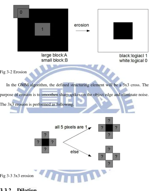
3.3.1 Erosion
Erosion[16][17] is a basic nonlinear operation in the morphological image processing. To perform erosion on an image A, we have to define structuring element B in the same time. If B can be completely contained by A in a location, than the output of this location will be logical 1, otherwise, the output will be 0. This is shown in Fig 3-2.
Fig 3-2 Erosion
In the GMM algorithm, the defined structuring element will be a 3x3 cross. The purpose of erosion is to smoothen sharp spikes on the object edge and eliminate noise. The 3x3 erosion is performed as following.
Fig 3-3 3x3 erosion
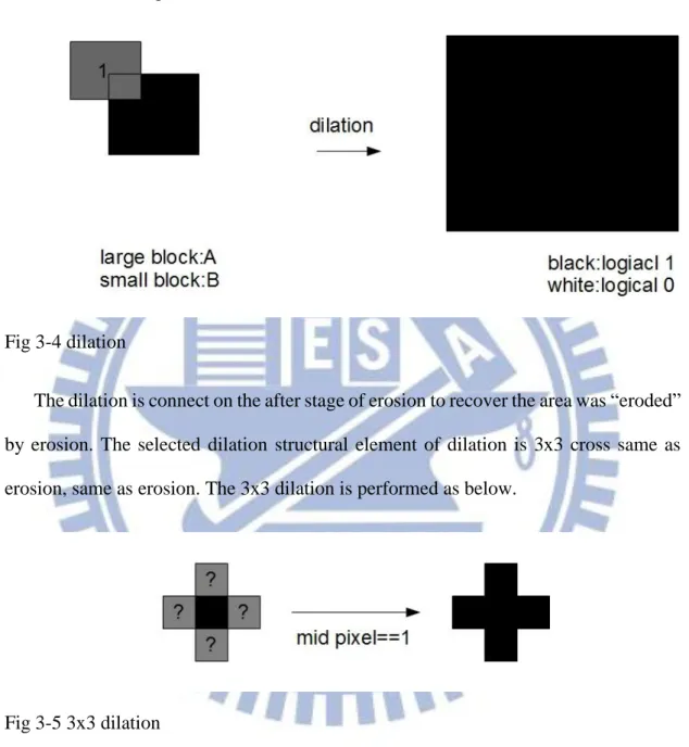
3.3.2 Dilation
On the other hand, dilation is another basic operation in morphological image processing, having a nearly opposite effect to erosion, which adds the pixels being eliminated back.
Again, start from structuring element, if a location of A can be covered by any part of B, then the output of this location will be logical 1, otherwise, the output will be 0. This is shown in Fig 3-4.
Fig 3-4 dilation
The dilation is connect on the after stage of erosion to recover the area was “eroded” by erosion. The selected dilation structural element of dilation is 3x3 cross same as erosion, same as erosion. The 3x3 dilation is performed as below.
Fig 3-5 3x3 dilation
3.3.3 Connected Component Labeling
After erosion and dilation, the noise is filtered and the objects are smoother on the edge. Then we assume that region enclosed by a line is an object. Connected Component Labeling(CCL) labels same number on the pixels of same region, and thus we can process these objects separately.
In the field of computer vision, the fast methods realizing CCL has been a popular researching topic[18][19], because the realization needs tedious pixel scans and they are intensive in computational costs. In the Chapter 4, we proposed an alternative method to replace CCL to meets the requirements and fit the hardware design better.
3.3.4 Object Classification
The binary images are being partitioned to several regions after CCL, and we will assume those regions are individual objects. The next step in the foreground object recognition is to classify each object. In the implemented version, there will be only moving or still object type available, but extra type such as shadow could be added.
For an object in the current frame, if we can find an object on the same location in the last frame, the object will be classified to a still object. In contrast, if nothing can be found on the location, which indicates the object may be moved or disappeared, then the objects will thus be labeled as a moving object.
3.4 The Pseudo C-Code
The details of each stage of the algorithm has been shown. This section will list the main flow in pseudo C-code.
Pseudo C-code:
//phase 1: check match condition for(x=0;x<IMAGE_WIDTH;x++){ for(y=0;y<IMAGE_HEIGHT;y++){ for(g=0;g<GROUP_NUMBER;g++){
for(ch=0;ch<CHANNEL_NUMBER;ch++){
//the match condition has been discussed in section 2.3 and section 3.2 } } foreground(x,y)=check_pixel_match(match); } }
//phase 2: object extraction and type classification
erosion(foreground); //do erosion and dilation twice to reduce the noise
erosion(foreground); dilation(foreground); dilation(foreground);
connected_component_labeling(foreground); //connect the foreground pixel
invalidate_small_object(foreground); type_classification(foreground,type(x,y)); //phase 3: update for(x=0;x<IMAGE_WIDTH;x++){ for(y=0;y<IMAGE_HEIGHT;y++){ for(g=0;g<GROUP_NUMBER;g++){ for(ch=0;ch<CHANNEL_NUMBER;ch++){ model(x,y,g,ch)=model_update(model(x,y,g,ch), in(x,y,ch),type(x,y)); } } } }
//phase 4: output results
Chapter 4 Hardware
Implementation
4.1 Hardware Oriented Algorithm
The targeted algorithm is a software based algorithm and not realistic to be implemented in the ASIC design. We made some modifications to the algorithm in the sense of hardware implementation.
4.1.1 Block based method in GMM background subtraction
Because the size of video is increasing rapidly, memory bus bandwidth is a bottleneck that most video algorithm must to deal with it. Insufficiency of memory bus bandwidth between chip and external memory, buffered data are stuck when store to and load from memory. In order to decrease the frequency of accessing, we cache the data are soon to be reused in the chip instead of storing back to external memory and load it back. There is another advantage to include such internal memory in the design. Irregular memory assessing increases the delay of each accessing to memory. The addresses have become regular after include such internal memory .The original and modified version of accessing is shown in Fig 4-1 and Fig 4-2.
Fig 4-1 original timing of memory
Fig 4-2 modified version of timing in the memory
Internal memories are major part of chip area. By reducing the internal memory capacitance, the area of memory can also be reduced and thus reduce the size of whole chip. In our original algorithm, temporal data have to be buffered for until end of whole frame, requires a large memory area. For above reason, we partition the frame to blocks, all data have to be buffered until a block finishes instead of a frame.
The input was read in the raster scan order in the original algorithm. In the modified version, the input was read block by block and in raster scans order in each block. In the original version, the object information was buffered until the end of the frame. In the modified version, object information had to be concluded and pass to next block in the end of every block. There might be some error occurs in this early determination step. Fig 4-3 and Fig 4-4 briefly explain the difference between the original version and the modified block based version algorithm.
The block size is an important parameter that affects performance of the algorithm and size of the chip. Generally, the choosing of block size depends on the type of input pattern. Because in the step of small object invalidation, the chip has to distinguish noise from object, so block edge width must larger than the smallest object in the input pattern. The following table shows the relationship between internal memory needed and block size. We will discuss this topic again in the section 4.1.5.
Block Size Without Block (HD) Without Block(VGA) 64x36 32x24 20x15 Memory Size 132.7Mbi t 19.7Mbit 147.46 Kbit 49.2Kb it 19.2Kb it
To summarize, the modification regulates the address for a better memory bandwidth and the chip area can still be small thanks to the block partition. Following sections will discuss how to modify the algorithm to block based version and in the meanwhile minimize the loss.
Fig 4-3 pixel processing order in the original algorithm
Fig 4-4 pixel processing order in the modified algorithm
4.1.2 Erosion and Dilation
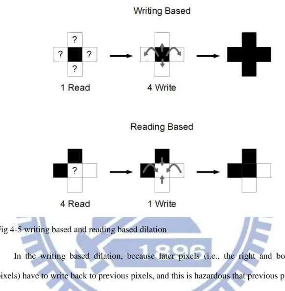
Reading operations are easier than write operations in memory scheduling, because changes in the reading order would not change the result. The dilation operation introduced in the Chapter 3 was writing based process. It is desirable to
modify such writing based process to reading based process. The following figure shows the difference between these two processes.
Fig 4-5 writing based and reading based dilation
In the writing based dilation, because later pixels (i.e., the right and bottom pixels) have to write back to previous pixels, and this is hazardous that previous pixels being read before last write (RAW, read after write hazard). When it comes to the reading based dilation, every pixel is ready for reading request from next operation, which reduced the RAW hazards. There’s an extra advantage to implement reading based dilation. After the modification, dilation is closer to erosion in terms of hardware. Both of them read information from 4 neighbor pixels, make decision and write to the center pixel. The similarity makes it easier to schedule the data and keeping the flexibility of pipeline operation of them in the same module.
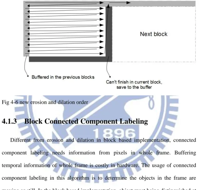
The erosion and dilation step needs only information of left, right, top and bottom pixel, not whole frame. As a result, it is easier to split erosion and dilation into blocks. The only change is the need of buffer to store the information at the edge of blocks. The following figure shows how this is block based implemented.
Fig 4-6 new erosion and dilation order
4.1.3 Block Connected Component Labeling
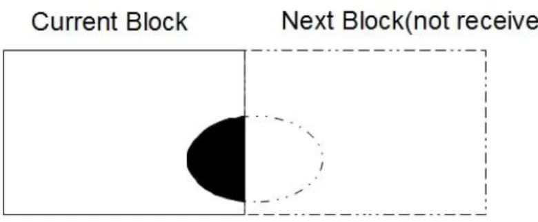
Different from erosion and dilation in block based implementation, connected component labeling needs information from pixels in whole frame. Buffering temporal information of whole frame is costly in hardware. The usage of connected component labeling in this algorithm is to determine the objects in the frame are moving or still. In the block based implementation, object must being distinguished at the end of each block rather than end of a frame. This requires a method to determine the object type before the shape of the object is completely received. Fig 4-7 shows what the method should do.
Fig 4-7 problem encountered in the connected component labeling
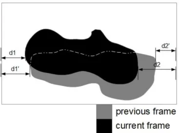
For the ellipses object in the figure, the original algorithm could make decision after the ellipses is completely received. In the block based algorithm, the chip has to make decision with incomplete object information (the black area). We proposed a method to solve this problem by mark the left and right edge of the object in the blocks. When compare to previous frame, if one of the edges moved more than a given threshold (this threshold value is pattern dependent and selected by experiment), then this block will be marked as a moving block. In the other hand, if the difference is less then the threshold, this block would be marked as a still block. Fig 4-8 shows the method.
Fig 4-8 modified version of connected component labeling in a block
Because our block is so small comparing to objects, there are a lot of blocks fully covered by object. Our algorithm proposed will be failed to deal with such blocks. Because the left edge and right edge of the object in the block will always be same as the block edges(Fig 4-9). In order to deal with this condition, the block will tell neighbor blocks if there is an object on the edge (having more than a given number of pixels lie on the edge). If on the both edge of neighbor blocks have an object, these two blocks are called connected. Connected blocks share the same block type. Fig 4-10 shows the modifications. Fig 4-11 shows how this problem can be solved by this modification.
Fig 4-9 problem encountered in the modified version of connected component labeling
Fig 4-11 type inherit in the connected blocks
If the object to deal with is simple (like the ellipses shape), this method goes well. When it comes to more complex shape or moving direction of objects, this method might be failed. Here’s some example.
1) More than 1 object appears in a block.
Fig 4-12 more than 1 object in a block
Take Fig 4-12 for example, this is a connected block that connect left and right neighbor. The type of this block will be same as its left block, and wrongfully classify the right block. This will result in wrong type decision in the right object and blocks connect to the block.
Generally, isolated object moves toward different direction, indicate the condition of “more than one object appears” will not take effect for too long. Once they can be separated to two different blocks, this problem then diminished. This problem indeed causes the instability to the system. Wrong type decision causes wrong background updating speed. In some test condition, it would be really fetal, but it is not a general condition in a day life as well as in our application.
2) Blocks failed to connect because of lacking of “future pixels”
It is shown in Fig 4-13, all of the blocks occupied by the object should be connected and shares same block type.
Fig 4-13 object in the different blocks but those blocks failed to connect
The information of whether to connect is received after the top-right block’s decision making, and then the system fails in this case. This appears when both condition holds:
Only the top-right blocks will be affected.
The edge with sharp spikes.
Apparently, these conditions would not hold for too long, we might take this problem optimistically. Most of time, the condition holds because the noise from the previous stage or simply from the video source, so they would not exist for too long, and most of all they are not removable in the Connect Component Labeling stage.
3) Object edge goes to a direction hard to connecting.
Fig 4-14 a direction of object hard to connect
In the Fig 4-14, these three blocks should have been connected but failed. Because when the decision making of top right block, it lacks the information of other two blocks that is necessary for correct decision. When type1 and type2 are different, the controversy exists in bottom right block.
This is a variant version of bug from example 2), previous blocks lacks the information of future pixels. The difference is example 3) exists whenever object edge goes the direction from top-right to bottom-left – very common in any type of video. Worst of all, this phenomena appears most in large objects indicates that the later blocks will connect to this wrongfully decide block, and propagate to the end of this object. However, this condition exists not at certain part of the object but exist randomly, because even if the algorithm has the chance to face the controversy, it still has the chance to make a right guess of type, eliminating the controversy. So such phenomenon will be well distributed to whole object. Whole object shares the same error is much better than only some certain part of object suffers. In our application, we have not seen major drawbacks at the output from this phenomenon. Here is a possible modification for other applications that really suffers from this phenomenon. First, the system should detect the possibility of such phenomenon and skip this block. Then, while the future pixels this block needed is ready, the system will goes back to the skipped blocks. This may be work to fix this problem, but it changes the data schedule pull the memory I/O speed down and increased the hardware complexity. So we will not use it in our algorithm.
In this section, we proposed an algorithm as an alternative to classical Connect Component Labeling, did some modification, and found some problem of it. It works in most conditions and needs only some corrections in certain patterns.
The last part of this section will be a test sample from ICU video. It is a man on the sickbed struggling to pull the equipment out of his body.
Fig 4-15 example of a frame of comparison between two versions
The black areas are object detection mismatched part with the original algorithm, the gray one are matched. The numbers means that the black area near by is caused by the examples of error of the number. As mentioned above, the 1)’s appears when multiple object exists in same blocks. They are most noise caused by the pattern of the cloth, by the way. 2) appears at the top right part of the object, the object is not a realistic object but a residue shadow left by his moving head. Real object will be smoother at the edge. For 3)’s it appears at the top-right to bottom-left edge, and propagate to the end of the block, and as mentioned above, the black area will change with other part of the object alternatively with frame change. As the result, the phenomenon is not obvious at the output stage.
4.1.4 Model Data Compression
The aim of this block-based version algorithm is to increase the memory I/O speed, it is also important to reduce the data transmit through the memory. Videos are usually highly spatially correlated. It is feasible to take advantage from this feature to reduce the size of data. From a previous research[23], the precision of model data is 32 bits or above is the best for performance. We will stay in 32 bit data for computations in chip, but when it comes to memory I/O, 32 bits are a large number not realistic to transmit. To deal with this, we take advantage from the correlation of data and reduce the data size for transmitting through data compression technique. We choose a fixed
length compression algorithm “Minimum-Maximum Scalar
Quantization”(MMSQ)[20] for simplicity. It is a general purposed data compression algorithm highlighted low computation requirement and fix length coding with decent compression performance. With those features above, MMSQ is really feasible to be an assisting part of a system[21]. With these features of MMSQ, we select it as model data compression algorithm.
Weighting data are the hardest part in the whole flow because of the longest data path and irregular timing. In the meanwhile, the weighting data size is only 16% in total model data. Therefore, we will not compress the weighting for hardware simplicity.
The following paragraph will introduce main ideas and steps of MMSQ[21].
Despite of the fact that model data requires 32 bits to process, because of the spatial correlation, the difference between neighbor pixels are usually extremely small in comparing to the magnitude of itself. If we find the range of the values in a given area ( i.e., find the Maximum value and Minimum value), and this range is small
enough that we can store this value with shorter code length but reach same precision, thus the shorter output code length. This is the key idea of MMSQ. Fig 4-16 shows the idea about MMSQ. It is clear that the dynamic range of inputs are phenomenally decreased by only store the difference between input and the group minimum. The 14 bits in the figure is the compressed code length we selected will be discussed later.
Fig 4-16 dynamic range of original and compressed version
Minimum-Maximum Scalar Quantization(MMSQ) encodes inputs in following steps:
1) divide successive inputs into groups ( 16 inputs as one group in the original paper).
2) for a group, find the minimum and maximum sample and the difference between them.
Q = (maximum-minimum) / 2n
where n is the output size for each input.
4) divide the difference between input and the minimum value by Q.
Quantized input difference = (input-minimum)/ Q
5) transmit quotients in 3. and necessary headers.
We select 14 bits as quantized output size because the system was scheduled to load all data in a pixel within 2 load operations. Each load operation in the memory loads 64bits data from the memory. We have 3 color channels and 3 group of color to load from the memory, 9 numbers in total. As a result, the compressed size of data is set to:
222
.
14
3(groups)
*
)
3(channels
2(times)
*
load)
per
64(bits
(4-1)The output size in bits after rounding off : 14bits.
Decoder is the reverse of the encoder and only steps will be listed.
Steps of MMSQ decoding:
1) load the Q-factor and the minimum.
2) get a input and multiply by Q, the result is the difference in the original scale.
3) add the difference from 2) to the minimum. 3) is the decoded number for the input.
4) load next input until a group is decoded, back to 2).
5) after a group complete, go to 1) for next group.
4.1.5 Invalidation of Small Objects
There is always noise in the video being recognized as objects ( Generally, they are moving objects), cause false alarm in the output stage. In the original algorithm, it invalidates small objects with the information of object size from Connected Component Labeling. When it comes to the block based version, we can no longer do such invalidation after complete object information because we have to finish at the end of blocks. The block size was same as the smallest object allowed, in order to distinguish object from noise. Unfortunately, objects will not always locate at the center of the block. They locate cross the block edge most of the time, so we can’t conclude all of the objects at the end of a block. So after the block based Connected Component Labeling, the result return to the system will buffer for the length of next block, check if the object is long enough to be validated.
In summary, this is a simplified version of the original algorithm, for the timing requirement of hardware. In the original version, because objects can be any arbitrary length, it is not realistic for system to wait for the result from Connected Component Labeling. On the other hand, data from only one block is not capable to invalidate noisy objects, we thus buffer for one more block.
When blocks are horizontally connected, they changes the information to determine whether the object is an object or noise. Note that the size of smallest allowed object depends on the test pattern, and the maximum size allowed is same as block edge width. Fig 4-17 shows the processes in this section.
Fig 4-17 demonstration of small object invalidation
In our medical monitoring application, we will apply the system to process a video of whole human body. The following figure analyses which block size is feasible under this application.
In this example, the frame is being divided into 30*30 blocks. The dimension of each block is 64*36 pixels. The example is filtered by the original algorithm that small objects are invalidated. Remaining objects are equal to are slightly bigger than the block size under this configuration. When we set the invalidation threshold equals to the block size, the block based version can provide similar function to the original one.
4.2 Simulation Results
In the last chapter, a series of modifications for hardware implementation has been proposed. A comparison between the original algorithm and the proposed algorithm on the sickbed video will be shown in this chapter. (Fig 4-19, Fig 4-20, Fig 4-21 and Fig 4-22) The meaning of each block in the video is shown below:
Test Video Block Based
Fig 4-19 result (FRAME=175, 5.83sec)
Fig 4-21 result (FRAME=215, 7.16sec)
The video is recorded in 30 fps, VGA resolution. In Fig 4-19 the patient suddenly moves his hand, causing a series of alarm (white area in the binary images). Generally, sudden actions of a patient indicate potential dangerous accidents, such as the patient feels discomfort or attempts to pull the plugs and should be aware by people.
The alarms in this video are mostly ghost images left by body and the movement of strip on the shirts is hard to tell which algorithm is better. Some important observations are given below:
1) The modified algorithm is more sensitive to new objects, and lower miss rate is desired in the field of hospital surveillances for safety.
2) The modified algorithm is noisier. This drawback is caused because of block operation and is hard to eliminate. Fortunately, a major part of these false-positive are from the edge of body, and these false-positive will not severely affect the performance.
3) The false-positives are eliminated in the almost same speed of both versions. None of the defects will last for too long in the modification.
4) The shadow of the pillow causes a large area of false detection. This is mainly because of the removing of shadow detection. The shadow detection had been removed to reduce the complexity. It is needed to take care of the impact on the successive stage and find corresponding solution.
In conclusion, we simplify the original tedious algorithm both in timing and in hardware costs. The modified version still meets the requirements despites of the defects.
4.3 Architecture
So far, we introduced an algorithm for medical monitoring, and made modifications for hardware implementation and compared the results. The next section will be the architecture of a hardware design about the modified version of GMM background subtraction algorithm.
4.3.1 Top Level
Fig 4-23 is the block diagram of whole design.
This design can be separate to two parts. They are the background part and the foreground part. The background part includes the DRAM at the top, MMSQ decoder, the update and MMSQ encoder. The rest is the foreground part, include classification, erosion and dilation, Connected Component Labeling (CCL) and weight update. The background part is only responsible for adapting the system to the input video as most of GMM algorithm do. It is simple in the scheduling thanks to the short data path. Unfortunately, this part is hardware heavy because it processes the raw 32bits model data. The divider and the multiplier account for about 70% area of the system. The foreground part, on the other hand, has only a few gates in hardware, but more complexes in the scheduling.
At the beginning, all of the data of current pixel will be load from DRAM and decoding. The next, do classify to decide this is a foreground or background pixel. The background part can start update and store to DRAM after classification stage. For the foreground part, the weighting will be stored in internal SRAM and the foreground/background information will be sent to the erosion, dilation and Connected Component Labeling to find the detail information about the foreground (i.e. objects). After the CCL stage, the learning rate of current pixel is determined, and then the buffered weighting will load from internal SRAM for update, and then store to weighting DRAM.
4.3.2 The DRAM Configuration
The model data are stored in 3 different memory banks. The mean, variance and the weighting will be stored individually. Under this configuration, both reading and writing of this memory will be in burst mode. The memory bandwidth will increase rapidly under burst mode. The arrangement of pixel in the memory is block based order.
4.3.3 Erosion and Dilation
The input of erosion and dilation is 1 for foreground and 0 for background. The section 4.1.2 mentioned the need of buffering the block edges for erosion and dilation in the neighbor block. Thus, Erosion or Dilation core is wrapped with a buffer. The wrapper is responsible for the switch of input and data buffer. Fig 4-24 shows the Erosion and Dilation with corresponding wrapper.
Fig 4-24 top of erosion and dilation
Because of the modification of dilation in section 4.1.2, both Erosion and Dilation shares same wrapper and scheduling. Fig 4-25 and Fig 4-26 shows the schedule of pixels in blocks and Fig 4-27 and Fig 4-28 shows the architecture of the core.
Fig 4-25 erosion/dilation wrapper (1)
Fig 4-26 erosion/dilation wrapper (2)
Because of the lacking of data at the block edge, the size of input data of the core should be two columns and two rows more. The extra data needed is fed from the buffer(shown in Fig 4-25), and thus the amount of input data is same as output
data(Fig 4-26)—easier in hardware design, no buffers needed between stages. The gray region of Fig 4-26 are data needed to be buffered for block at next column and next row.
Fig 4-27 architecture of erosion/dilation core
Fig 4-28 data in the buffer of erosion and dilation
Fig 4-27 is the architecture of the core. It consists of a shift register having a length equals to two rows in block (Fig 4-28). There will not be any output until the DFFs are filled with inputs. After the DFFs are filled, the core takes data from the five pixels marked on Fig 4-27(Q1 to Q5) and do the corresponding bit operation (AND operation for Erosion and or operation for Dilation).
Connected Component Labeling consists of two parts: the CCL_main and the CCL_ buffer. The CCL_main counts the length of object in pixels, get the position of object edge and make decisions about the type of objects and the CCL_Buffer buffers the output from CCL_Main for the period of one more block to wait for the final decision by CCL_Main. Fig 4-29 shows the architecture.
Fig 4-29 architecture of connected component labeling
The output and type output will connect to weight update, the weight update chooses corresponding learning rate from the block type, and do the update from the result of output.
4.3.5 Compression
The MMSQ algorithm needs a buffer to keep a period of data, controls to find the maxima and the minima, and a divider, which really large in area, to do the quantization.
Fig 4-30 architecture of MMSQ encoder
There are 18 sets of MMSQ_ENC and MMSQ_DEC in the top level, Fig 4-30 is only one set of MMSQ_ENC for simplicity.
The DFFs buffers the inputs in the first state of FSM. In the next, the combinational circuit will find the maximum and the minimum from the buffer then evaluate the Q-factor. The minimum and the Q-factor will be outputted as soon as evaluated. The Q-factor will be sent to the divider as divisor, too. The final state is to load the inputs from buffer in order, send to divider as dividend. The quotient is the output.
In order to meet the timing requirement, the compression used three 6-latency sequential divider, which generates an output for every 2 cycles in the encoder.
The design of decoder is easier, no input buffer required for decoder. In the mean while, the multiplier in the decoder is fast enough on the timing, no parallel nor
sequential buffering required, so the area of decoder is much smaller than encoder. Fig 4-31 shows the design of decoder.
Fig 4-31 architecture of MMSQ decoder
4.3.6 Update
Updating is a series of multiplication and addition, thus the block diagram will not be shown here. The hardest work in updating is to determine the bitwise precision of each variable. The 32 bits precision is suggested in the previous section, so the work here is to guarantee the correctness of the 32-th bit.
Here is a method to estimate the precision needed for each variable. We can consider a variable A’ with infinite precision as a finite precision variable A with a random noise n from bitwise truncation.
A=A’+n , n<2-bits
If a product P=A*B needs a precision of first k bits, we can get the function:
P = P’+np = A*B = (A’+na)*(B’+nb) = A’B’ + A’*nb + B’*na + na*nb
P’=A’B’ is the original multiplication without any loss, will be eliminate from both side of the equation, the na*nb is much smaller than other terms and will also be
eliminated. Then the equation after elimination will be:
A’*nb + B’*na = np<2-32
If the information of A’ or B’ is known (by experiment or any method), then we can find max na and nb allowed by equation above. Since the upper bound of na and nb is set, the precision needed for A and B then determined.
For example, if we performed the multiplication: mean *α, where α=0.025 is the learning rate of mean. Note that we still need to represent α in finite digital variable, so there will also be an error in this process.
Start with the equation:
P’+np = m * α (m=mean)
Then perform the steps as above:
P’+np = ( m’ + nm ) * ( α’ + nα )
= m’α’ + m’nα + α’nm + nmnα
Eliminate in the both side of equation: m’nα + α’nm =np < 2-32
then
m’nα < 2-32 and α’nm<2-32
Start with the latter, α’ will be really close to α with only a finite error, and α’ ≈0.025 nm< (2-32 /α’) = 2-26.678
A variable with 26 bits guarantees a precision of 2-27 , we can select 26 bits for variable mean.
And the former:
Since we know the input will be an integer less than 256: m’nα< 255*nα < 2-32
and
nα < 2-39.994
same as mean, we then select 39 bits for α.
The precision of other variables can be derived in same technique.
There’s a difference between the multiplier in updating(i.e., the learning rates) and in MMSQ_DEC, because the multiplier in update are known , so it is simply bit shifting and additions, not real multipliers as in MMSQ_DEC.
4.4 Gate-Counts
The design has been implemented under TSMC 90nm process by Verilog Hardware Description Language. Both VGA and Full-HD resolution have been tested on 30 FPS. The following table shows the area of each part.
List of Chip Area (in k-gates)
VGA Full-HD Memory Encoder 275.13 276.51 Memory Decoder 35.61 35.66 Total(Compression) 310.74 312.17 Erosion 23.59 72.01 Dilation 23.59 72.01 Update 16.03 16.03 Weight Update 4.77 4.77 Total(Design) 67.98 164.82 Total 378.72 476.99
The pipelines and the hardware parallelism are applied under the specification of Full-HD version. As a result, downscaling the same design to implement VGA version will only slightly reduce the area. The major area change between the versions is the row buffer in the Erosion and Dilation, which do not have much to do with clock speed.
The next table compares our proposal to other similar approaches.
The proposed algorithm provides Full-HD resolution and utilizes the foreground information in background update that outperforms other algorithms in terms of resolution and performance. However, the gate count is much lager than MBM algorithm because of the frame size. The increased stableness and the sensitivity are worth the high gate count.
Peng[4] Genovese &
Napoli [5] Proposed
Algorithm MBM GMM+Denoising Block-GMM
Technology
(Board) TSMC 0.18um Xilinx xc5vlx50 TSMC 90nm
Gate count(Slices) 14.4K 1179+291Register 168.42K
Resolution CIF Full HD Full HD
In the future, the design will be downloaded to XUPV5[22] and integrate with PC for real test.
Chapter 5 Conclusion
There are two major contribution of this thesis. In the first half of chapter 4, a modification of the algorithm in chapter 3 has proposed. Another half of chapter 4 proposed an architecture implement the whole algorithm.
The algorithm is not feasible to be implemented directly without any modification because hardware difficulties, thus, hardware oriented version being proposed. We divide the frame into blocks to avoid extra delays from the memory, and a series of modification has been done to the original algorithm. A block based erosion and dilation with wrapper is proposed to replace the original erosion and dilation. In the meanwhile, a block based connected component labeling is proposed to replace the original one, and the results of simulations show the block based CCL fits our application as well. In addition, a compressor has been added between the chip and memory to save the memory bandwidth further.
The requirement of the chip is work on VGA resolution and 30fps. Higher resolution Full-HD is also tested. Further requirement on the resolution or one chip for multiple camera are possible in the future.
References
1. C. Bishop., “Pattern Recognition and Machine Learning”, pp.423-455, 2004. 2. G. J. McLachlan, T. Krishnan and S. K. Ng., “The EM Algorithm” Center for
Applied Statistics and Economics (CASE), Humboldt-Universität Berlin, 2004. 3. Jensen, J. L. W. V., "Sur les fonctions convexes et les inégalités entre les valeurs
moyennes". Acta Mathematica 30 (1): 175-193., 1906
4. R. J. A. Little and D. B. Rubin., “Statistical Analysis with Missing Data” Wiley Series in Probability and Mathematical Statistics. New York: John Wiley & Sons. pp. 134-136. ISBN 0-471-80254-9. , 1987.
5. M. Piccardi., “Background subtraction techniques: a review”, 2004.
link:http://www-staff.it.uts.edu.au/~massimo/BackgroundSubtractionReview-Pic cardi.pdf
6. Y. Benezeth., “Review and evaluation of commonly-implemented background subtraction algorithms” International Conference on Pattern Recognition, pp.1-4, 2008.
7. A. M. McIvor., “Background Subtraction Techniques”, Reveal Ltd , Auckland, New Zealand, 2000.
8. C. Stauffer and W.E.L Grimson., “Adaptive background mixture models for real-time tracking”, In Computer Vision and Pattern Recognition, vol. 2, pp. 252–258, 1999.
9. W.E.L Grimson, C. Stauff er, R. Romano, and L. Lee., “Using adaptive tracking to classify and monitor activities in a site”, In Computer Vision and Pattern
Recognition, p.p 22–29, 1998.
10. Z. Zivkovic., “Improved Adaptive Gaussian Mixture Model for Background Subtraction”, In Proc. ICPR, 2004.
11. C. R. Wren, A. Azarbayejani, T. Darrell, and A. Pentland., “Pfinder: Real-time tracking of the human body”, IEEE Trans. on PAMI, vol. 19, no. 7, pp. 780–785, 1997.
12. D. M. Titterington., “Recursive Parameter Estimation Using Incomplete Data”, Journal of the Royal Statistical Society. Series B (Methodological) Vol. 46, No. 2, pp. 257-267, 1984.
13. Z. Zivkovic, “Recursive Unsupervised Learning of Finite Mixture Models”, IEEE Trans. on PAMI, VOL. 26, NO. 5,pp.651-656 2004.
14. H.H Lin, J.H Chuang and T.L Liu., “Regularized Background Adaptation: A Novel Learning Rate Control Scheme for Gaussian Mixture Modeling”, IEEE Transactions on Image Processing, vol. 20, pp. 822 – 836, 2011.
15. D. S. Lee, “Effective Gaussian mixture learning for video background
subtraction”, IEEE Trans. Pattern Anal. Mach. Intell., vol. 27, no. 5, pp. 827–832, May 2005.
16. Erosion online tutorial 1:
http://www.cs.auckland.ac.nz/courses/compsci773s1c/lectures/ImageProcessing-html/topic4.htm#erosion
17. Erosion online tutorial 2:
http://www.inf.u-szeged.hu/~ssip/1996/morpho/morphology.html
18. L.D. Stefano and A. Bulgarelli., “A Simple and Efficient Connected Components Labeling Algorithm”, ICIAP Proceedings of the International Conference on Image Analysis and Processing, pp.322, 1999.
operations in the course of forward raster scan followed by backward raster scan” 15th International Conference on Pattern Recognition, vol. 2, pp.434-437, 2000
20. A. D. Gupte, B. Amrutur, M. M. Mehendale, A. V. Rao, and M.Budagavi., “Memory Bandwidth and Power Reduction Using Lossy Reference Frame Compression in Video Encoding”, IEEE Transactions on Circuits And Systems For Video Technology, vol. 21, no. 2, Feb. 2011
21. S.W. Hsu and T.S. Chang., “A low complexity speech coder for binaural communication in hearing aids”, ISCAS, pp. 2801 – 2804, 2012.
22. Details specification of XUPV5 could be found in: http://www.xilinx.com/univ/xupv5-lx110t.htm
23. C.W. Huang., “Investigation of Fixed-Point Implementation of GMM”, 2011 24. I. Haritaoglu, D. Harwood and L. S. Davis., “W4: Who? When? Where? What? a
real time system for detecting and tracking people”, Third Face and Gesture Recognition Conference, pp. 222-227 1998.
25. D.Z. Peng., “VLSI Design for Foreground Object Segmentation with Labeling and Noise Reduction Mode in Video Surveillance Application” a thesis of Department of Electrical Engineering National Central University 2009. 26. M. Genovese, E. Napoli., “FPGA-based architecture for real time segmentation

![Fig 3-1 main steps of background maintain [14]](https://thumb-ap.123doks.com/thumbv2/9libinfo/8270786.172722/21.892.136.755.243.889/fig-main-steps-background-maintain.webp)