動態VoWLAN傳送速率的估計與調整

(1)

I

動態 VoWLAN 傳送速率的估計與調整

Link Rate Estimation and Adaptation

for VoWLAN with Mobility

研究生：李彥輝

Student: Yann-Huei Lee

指導教授：林盈達

Advisor: Ying-Dar Lin

國立交通大學

網路工程研究所

碩士論文

A Thesis

Submitted to Institute of Network and Engineering College of Computer Science

National Chiao Tung University in partial Fulfillment of the Requirements

for the Degree of Master

in

Computer Science and Engineering December 2007

Hsinchu, Taiwan, Republic of China

(2)

II

動態 VoWLAN 傳送速率的估計與調整

學生：李彥輝

指導教授: 林盈達

國立交通大學資訊工程學系網路工程研究所碩士班

摘要

當在具有移動性的無線網路傳輸環境之下，一直維持相同的傳輸速率不是隨時都適合的。太快的傳輸速率會導致封包遺失率攀升，太慢的傳輸速率則會讓單一個客戶端裝置占據過久的媒體使用時間導致其他用戶端無法傳輸資料。大部分的傳輸速率調整演算法都是考量以傳送的頻寬當作主要的衡量標準，但是像 VoIP 這類的應用軟體的需求和特質卻沒有被納入考量。因此在本篇論文中我們將會找出一個能配合 VoWLAN 的需求在有移動性的環境之下的傳輸速率調整演算法。我們除了使用 mean opinion score (MOS) 來當作衡量聲音傳輸品質的標準，我們還用 medium consumption (MC)來衡量介質被占據的時間。MC 是計算一個用戶端在完成其 VoIP 傳輸時的總時間中占據的百分比。所以我們提出的演算法 Voice Quality based AutoRate (VQAR) 來針對每個封包選擇可以有最小的 MC 且 MOS 在一定的品質(>3.5)的傳輸速率。從我們模擬的結果，ARF/AARF、 VQAR 和 RBAR 都可以達到所需要的 MOS 值，但是 VQAR 的 MC 分別比起 ARF/AARF 和 RBAR 低 11%和 27%。

(3)

III

Link Rate Estimation and Adaptationfor VoWLAN with Mobility

Student: Yann-Huei Lee

Advisor: Dr. Ying-Dar Lin

Institute of Network and Engineering

National Chiao Tung University

Abstract

When transmitting VoIP traffic over wireless medium under mobility conditions, using constant rate for transmission would not be suitable. Rates too fast would result in massive packet loss; rates too slow would result in high channel occupation by a single station. Most research on rate selection only considers throughput, but the characteristics of applications, such as VoIP, is not considered. In this paper, we estimate an adapt transmission rate for VoWLAN with mobility. Besides mean opinion score (MOS) for voice quality evaluation, we introduce a measure, medium consumption (MC), for channel occupation. MC is the percentage of channel time occupied by a station during its VoIP connection. We propose Voice Quality based AutoRate (VQAR) to select per packet transmission rate that minimizes MC while achieving the required MOS (> 3.5). From our simulation results, all compared methods ARF/AARF, VQAR and RBAR meet the required MOS, but VQAR has lower MC than ARF/AARF and RBAR by 11% and 27%, respectively.

(4)

IV

List of Figure

Figure 1. Pseudo code ... 7

Figure 2. MOS of different transmission rate under different distance ... 8

Figure 3. MC of different transmission rate under different distance ... 9

Figure 4(a). Sustainable Rate selection at different distance ... 10

Figure 4(b). Sustainable Rate selection at different SNR value ... 10

Figure 5. BER of different distance ... 11

Figure 6. Different algorithm’s MOS, MC, and transmission rate at different distance ... 12

Figure 6(a). Comparison on MOS ... 12

Figure 6(b). Comparison on MC ... 13

Figure 6(c). Comparison on transmission rate ... 13

Figure 7. Different algorithm’s MOS and MC with different velocity moving away from BS ... 15

Figure 7(b). Comparison on MC ... 15

Figure 8. Different Algorithm’s MOS & MC with different amount of MS nodes ... 16

Figure 8(b). Comparison on MC (summation of all MS nodes) ... 17

Figure 8(c). Comparison on MC (of single MS node) ... 17

Figure 9. MOS and MC of different codex at different distance (transmission rate = 24Mbps) ... 19

(6)

VI

List of Tables

Table 1. Comparison of rate adjustment algorithm ... 3 Table 2. MOS value to listener perception ... 4 Table 3. SNR vs Sustain Rate Selection ... 10

(7)

1

Chapter 1 Introduction

Transmission in wireless medium suffers more packet loss than wired. Unlike wired transmission using a single cable line, wireless transmission uses a shared medium. Interferences, such as white noise, distance fading, electromagnetic pulse, solar activity, radiations, etc., effects are much stronger in the open air than a single copper line. Although such packet loss can be recovered by retransmission mechanism of transport layer, but retransmission may not be acceptable by Real-time applications, such as VoIP, which need to be delivered within a limited time but is tolerable to some losses (not exceeding 1%). So transmitting delay sensitive real-time packets over a best-effort protocol would be a disaster. Therefore, how to maintain the quality of real-time VoIP traffic running over WLAN (VoWLAN) becomes a new issue.

Interference effect quality of voice transmission by distorting packets causes packet loss. The more packets dropped, the harder it is to reconstruct a complete replay, resulting in poor quality. In the PHY layer, changing modulation is a method to deal with interference. To compensate distortion, different modulation methods uses different amount of symbols to represent a bit, resulting in different speeds of transmission and different levels of tolerance to interference. The more symbols used, the easier the receiver could correct distortion caused by interference, but the slower the transmission rate is [1]. The modulation with the highest tolerance to interference would indeed guarantee a suitable quality, i.e. a sustainable rate, for voice transmission. Utilization, however, is not guaranteed if using the lowest when faster rates are available. The channel would be occupied by a single transmission longer if a lower rate is selected. The tradeoff exists between quality and utilization under different level of interference. Therefore, a rate adaptation method is needed to satisfy these two constraints.

To evaluate the transmission quality and utilization of a VoWLAN transmission, two metrics are needed: mean opinion score (MOS) [2] and medium consumption (MC). MOS

(8)

2

provides a numerical indication of the perceived quality of received media after compression and/or transmission. The MOS is expressed as a single number in the range 1 to 5, where 1 is lowest perceived quality, and 5 is the highest perceived quality. To evaluate the utilization of a mobile station when several clients share the same base station, medium consumption is used for evaluating the occupation percentage used by a station’s VoIP connection.

Therefore, our problem statement is to find and choose a most efficient sustainable rate which satisfies certain amount of MOS with minimum MC for VoWLAN transmission under mobile movements. When current rate becomes unsuitable, pick a better rate for retransmissions. NS-2 [3] is used for simulations to find out the most efficient sustainable rate. We use all possible rates run through all possible level of interference and measure their MOS and MC. Here we use signal to noise ratio (SNR) as a term for evaluating the interference since it is mainly composed by the degrading of transmission signal power with the environmental noise. So we measure the MOS and MC of every rate at every SNR. Most efficient sustainable rate selection would then be plotted by selecting the rate that is within an acceptable range of MOS with minimum MC at every SNR. Selection of initial and retransmission rate would then be based on this mapping of SNR to most efficient sustainable rate.

In the next chapter we’ll introduce other rate adaptation algorithms. Chapter 3 will introduce the evaluation and rate selection method, Voice Quality based AutoRate (VQAR), we used developed for VoIP traffics. Chapter 4 would be the result of our simulation with the method mentioned in chapter 3 and comparisons of VQAR with ARF, AARF, and RBAR. Chapter 5 will be the conclusion for this paper’s work and possible future works.

(9)

3

Chapter 2 Related Work

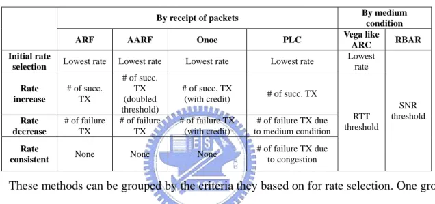
From the previous chapter, we know there’s a tradeoff between error toleration and transmission bandwidth, rate adaptation methods have been designed to find suitable rates for transmission. Table 1 is a comparison of 6 rate adaptation methods: auto rate fallback (ARF) [4], Adaptive ARF (AARF), packet loss classification (PLC) [5], Onoe [6], vega like audio rate control (ARC) [10], and Receiver-Based AutoRate (RBAR) [7].

Table 1. Comparison of rate adjustment algorithm.

By receipt of packets By medium condition ARF AARF Onoe PLC Vega like

ARC RBAR Initial rate

selection Lowest rate Lowest rate Lowest rate Lowest rate

Lowest rate SNR threshold Rate increase # of succ. TX # of succ. TX (doubled threshold) # of succ. TX

(with credit) # of succ. TX

RTT threshold Rate decrease # of failure TX # of failure TX # of failure TX (with credit) # of failure TX due to medium condition Rate

consistent None None None

# of failure TX due to congestion

These methods can be grouped by the criteria they based on for rate selection. One group depends on the success or failure of packet transmission. ARF and AARF adapt rate by decreasing transmission rate after certain amount of failure transmissions, and increase after a certain amount of successful transmissions. But AARF will double the amount of success transmissions needed to increase the rate in the next run if it fails to increase in current run. Onoe maintains a credit number which varies as the amount of success or failure transmission reaches a certain threshold. By this credit number, Onoe would decide to increase or decrease transmission rate. PLC increase and decrease rate like ARF, but it would further inspect the reason of failure and decrease rate when it’s due to medium condition and maintain current rate if it’s due to congestion. Another group of rate adaptation methods depends on phenomenon of the medium. Vega like ARC uses round trip time (RTT) for it’s metric in rate adjustment. Receiver-Based AutoRate (RBAR) adjust rate by determining the SNR value

(10)

4

where BER of a rate increases over to 10-5. The bounds of SNR value for each rate are

determined and rate selection would be based on this SNR threshold VS rate plotting.

The methods above were designed to carry data traffic, so throughput and bandwidth was their main concern. Quality of voice and medium utilization of VoWLAN traffic, however, wasn’t considered. In this paper, we would tend to find the most efficient sustainable rate for initial transmission and rate adaptation, satisfying the quality needed voice transmission and maximize utilization for VoWLAN traffic.

Chapter 3 Voice Quality based AutoRate (VQAR)

Our algorithm is based on a SNR to rate mapping function Rs(SNR). This function

guarantees the rate mapped from a certain SNR would be the rate that has MOS > 3.5 with minimum MC value. We will introduce our the way to get such function bellow.

3.1 Transmission quality & utilization evaluation metric

As mentioned in chapter 1, for evaluating the quality of a VoWLAN transmission, we used Mean Opinion Score (MOS), and Medium Consumption (MC) for evaluating utilization.

Table 2. MOS value to listener perception

MOS Quality Impairment

5 Excellent Imperceptible 4 Good Perceptible but not annoying 3 Fair Slightly annoying

2 Poor Annoying

1 Bad Very annoying

MOS is used for evaluating audio quality after encryption or transmission. It’s a rating score of 1 to 5 with 1 as the poorest quality and 5 as the best, as shown in table 2. The acceptable range for VoIP would be 3.5 ~ 4.2. Usually, MOS is calculated by letting nearly 100 people listen to the audio after encryption or transmission and give a score from 1 to 5 rating the quality of the audio they hear. The average of the result would be the MOS score for this certain encryption or transmission. The original method for MOS calculation is too expensive, so an artificial method called “E-model” [8] is develop to calculate MOS by

(11)

5

certain input variables. The E-model calculates a “R-factor” based on formula (1). A -Ie -Id -Is -Ro factor -R = (1) Whereas, mobility) (e.g., factor advantage : A coding) speech to due distortion signal (e.g., factor impairment equipment : Ie echo) (e.g., delay to due factor impairment : Id loudness) excessive (e.g., processing speech usly with simultaneo occur that impairment : Is noise) circuit side, either at noise room (e.g., factor ratio noise : Ro

Formula (1) could be simplify to (2) by import known values for Ro, Is, and A according to our simulation scheme.

Ie -Id -93.34 factor -R = (2)

Id and Ie could be calculated by extracting NS-2 simulation result. From this we could calculate the R-factor and transfer to MOS.

MC is a metric defined by ourselves for evaluating the capacity a single VoIP connection takes up. It’s likely to have multiple transmissions on the air at the same time within an access point; it would be best to have each transmission to take up lesser time in transmission and allow more time for other transmissions. Therefore, fully utilize the medium. We define MC by formula (3). time period connection VoIP period the in n applicatio VoIP a by occupied time MC= (3)

Smaller MC means less occupation of a session, which would be able to provide more service to more subscribers, and would also provide better utilization.

3.2 Voice Quality based AutoRate (VQAR)

Our approach is based on the most efficient sustainable rate vs SNR formula, Rs(SNR).

By measuring the MOS and MC of all possible rates at different mobility status, we could select the rate which has MOS > 3.5 with minimum MC. Then with the given relationship we use it as a reference for initial and retransmission rate selection in our proposed algorithm - Voice Quality based AutoRate (VQAR).

(12)

6 3.2.1 Most Efficient Sustainable rate discovery – Rs(SNR)

In order to estimate the influence of mobility, we use signal to noise ratio (SNR). By simulation, SNR can be calculated through free space propagation in outdoor environment. SNR is calculated by formula (4) and free space loss is calculated by formula (5).

) power noise / P ( log 10 SNR= × 10 r (4) 2 2 t r fd) (4 c P P π = (5) Whereas, (m) distance d 1/s) (Hz frequency f (m/s) light of speed c power signal er transmitt Pt power signal receiver Pr = = = == =

Noise is usually construct by thermal noise (i.e. white noise), which is a constant value. From (4) and (5), we could see that SNR variates with distance only. Therefore, it is safe to use distance to represent influence of mobility in an outdoor free space environment. And we could convert distance to SNR for a more general situation.

First, we set two stations separated by a known distance, from 1m to 300m, and let VoIP traffic sent from one station to the other. The VoIP traffic is simulated by putting a constant bit rate traffic flow to simulate G.729 codec. By changing the distance, we could measure the MOS and MC of a certain rate at different SNR. The process is repeated with other rates, and we could get a complete plotting of SNR VS MOS and SNR VS MC for different rates. The relation of the most efficient sustainable rate and SNR RS(SNR) could be plotted from the

graphs we got previously, by choosing the rate with MOS value in the acceptable range for VoIP (= 3.5~4.2) with the minimum MC. With this relation, we could use it for our initial and retransmission rate selection.

(13)

7 3.2.2 Initial and Retransmission rate selection

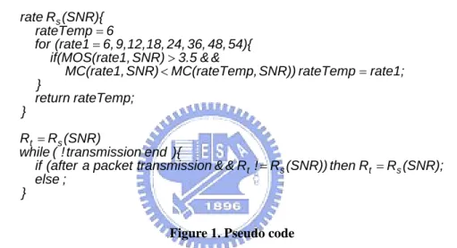
Rs(SNR) can be calculated by the pseudo code shown in Figure 1, once we calculated the

MOS and MC of each rate at different SNR, ie. MOS(rate, SNR) and MC(rate, SNR) respectively.

Initial rate selection is very forward. By measuring the current SNR value (denoted as SNR) and the SNR vs. most efficient sustainable rate mapping graph (denoted as Rs(x)) plotted previously. The selection of the initial rate, or the current transmission rate (denoted as Rt), would be the most efficient sustainable rate at the current SNR.

} ; else (SNR); R R then (SNR)) R ! R & & on transmissi packet a (after if ){ end on transmissi ! ( while (SNR) R R } rateTemp; return } rate1; rateTemp SNR)) p, MC(rateTem SNR) MC(rate1, & & 3.5 SNR) e1, if(MOS(rat 54){ 48, 36, 24, 18, 12, 9, 6, (rate1 for 6 rateTemp (SNR){ R rate s t s t s t s = = = = <> ==

Figure 1. Pseudo code

During transmission, we shall inspect if Rt is equal to Rs(SNR) per packet. If they are

different, we change Rt to Rs(SNR). Otherwise nothing is changed. The pseudo code is shown

in Figure 1. So as long as we select our transmission rate according to the RS(SNR) function,

we could guarantee the rate has MOS > 3.5 and minimum MC value.

Chapter 4 Simulation Results

4.1 Most Efficient Sustainable rate Rs(SNR)

According to the method mention in 3.2.1, the results of the simulations are shown in Figure 2, 3 and 4. Figure 2 is done by keeping the MS at different fixed distance, 1m to 300m, transmitting a UDP constant bit rate (CBR) traffic simulating the behavior of G.729 codec for

(14)

8

1000 packets and measure the average MOS value. From Figure 2 we could see that the voice quality drops rapidly when it exceeds the maximum transmission distance available. The MOS of 9Mbps drops earlier than 12Mbps, unlike the behavior of other rates. This is because 6 and 9Mbps uses BPSK modulation while 12, 18, 24, 36, 48, and 54Mbps uses QAM modulation. 0 0.5 1 1.5 2 2.5 3 3.5 4 4.5 0 25 50 75 100 125 150 175 200 225 250 275 300 325 350 Distance (m) MOS 6Mbps 9Mbps 12Mbps 18Mbps 24Mbps 36Mbps 48Mbps 54Mbps 54mb/s 48mb/s 36mb/s 24mb/s 18mb/s 9mb/s 12mb/s 6mb/s

Figure 2. MOS of different transmission rate under different distance

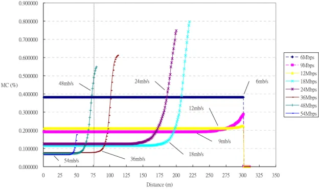
Figure 3 is simulated in the same situation as Figure 2, but we observe MC instead of MOS. The figure shows that higher rates have lower MC, but 9, 12, 18, and 24Mbps violate this fact.

(15)

9 0.000000 0.100000 0.200000 0.300000 0.400000 0.500000 0.600000 0.700000 0.800000 0.900000 0 25 50 75 100 125 150 175 200 225 250 275 300 325 350 Distance (m) MC (%) 6Mbps 9Mbps 12Mbps 18Mbps 24Mbps 36Mbps 48Mbps 54Mbps 18mb/s 6mb/s 12mb/s 9mb/s 24mb/s 36mb/s 48mb/s 54mb/s

Figure 3. MC of different transmission rate under different distance

With the results from Figure 2 and 4, we could decide the most efficient sustainable rate as shown in Figure 4(a). After we convert distance to SNR, we could get the results shown in Figure 4(b) and Table 3 for the distance/SNR to sustain rate mapping in our algorithm. This mapping guarantees the rate has MOS > 3.5 and minimum MC for current medium condition.

What would happen if we picked a higher or lower rate than Rs(SNR)? At 75m, for example,

Rs(SNR) = 36Mbps. If we pick a higher rate 48Mbps, MC is higher than 36Mbps (as shown in

Figure 3) and MOS is way lower than 3.5 (as shown in Figure 2). If we picked a lower rate 24Mbps, MOS is satisfied (as shown in Figure 2), but MC is still higher than 36Mbps (as shown in Figure 3).

(16)

10 0 10 20 30 40 50 60 0 50 100 150 200 250 300 350 Distance (m) Rate (Mbps) Rs (Mbps) 54mb/s 48mb/s 36mb/s 12mb/s 18mb/s 6mb/s 9mb/s

Figure 4(a). Sustainable Rate selection at different distance

0 10 20 30 40 50 60 1 10 100 1000 10000 100000 SNR rate(mb/s) Rs (Mbps) 6mb/s 12mb/s 18mb/s 9mb/s 36mb/s 48mb/s 54mb/s

Figure 4(b). Sustainable Rate selection at different SNR value

Table 3. SNR vs Sustain Rate Selection

Distance(m) SNR Rate (Mbps) >284 < 1.0518 6 252 ~ 284 1.0518 ~ 1.3452 12 167 ~ 251 1.3452 ~ 3.0632 9 78 ~ 166 3.0632 ~ 14.6415 18 50 ~ 77 14.6415 ~ 34.1714 36 39 ~ 49 34.1714 ~ 56.166 48 < 39 > 56.166 54

(17)

11

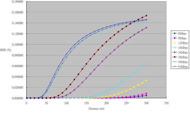
The reason we used MOS and MC for our main criteria instead of BER like other rate adaptation algorithm is because BER based algorithms are too conservative for VoIP traffic. Take RBAR for example, it guarantees the selected rate has BER < 10-5 although providing a satisfied MOS value, but has higher MC than VQAR (from the results of the following sections) since RBAR drops transmission rate earlier than VQAR to maintain a low BER. As we can see in Figure 5, BER increases faster as the transmission rate gets faster. However, phenomenon of 12Mbps having better MOS than 9Mbps, 18Mbps and 9Mbps has better MC than 24Mbps and 12Mbps, in Figure 2 and 3 are not shown in Figure 5. So using BER for VoIP traffic criteria is not completely suitable.

0.000000 0.020000 0.040000 0.060000 0.080000 0.100000 0.120000 0.140000 0.160000 0.180000 0 50 100 150 200 250 300 350 Distance (m) BER (%) 6Mbps 9Mbps 12Mbps 18Mbps 24Mbps 36Mbps 48Mbps 54Mbps

Figure 5. BER of different distance

4.2 Comparison of VQAR, ARF/AARF, RBAR

We compare the performance of our algorithm VQAR with auto rate fallback (ARF), advance ARF (AARF), and RBAR under three different situations: static MS with different distance to BS, moving MS at different velocity, and multiple node transmission.

(18)

12 4.2.1 static MS with different distance to BS

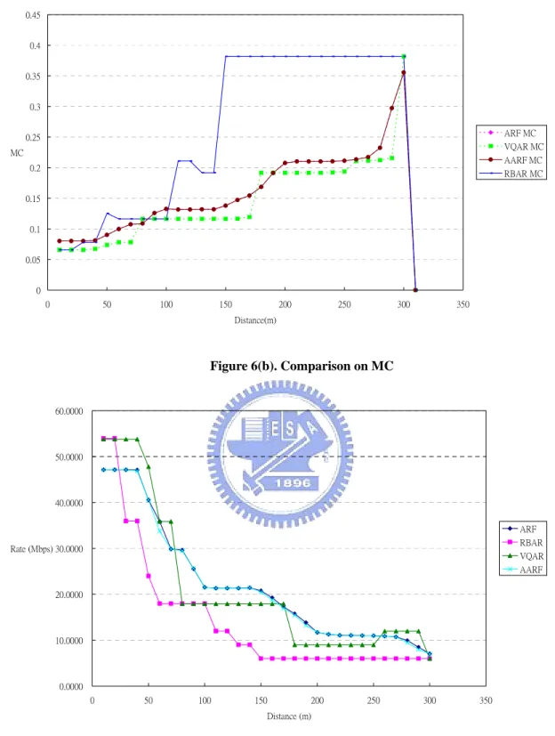
In the first scene, we put the MS at different fix distance and observe the MOS and MC value of ARF/AARF, RBAR, and VQAR. The simulation results are shown in Figure 6.

As we can see in Figure 6(a), MOS value of VQAR is just slightly better than ARF/AARF and almost the same as RBAR. However, this difference is not significance for human ear, since the MOS values are all slightly above four.

As for MC in Figure 6(b), VQAR is lower than ARF/AARF and RBAR in most of the distances. This is because VQAR could find the suitable rate with the lowest MC immediately, unlike ARF needs to start from the lowest rate increasing the transmission speed step by step until reaching the suitable rate. Although RBAR choose rate according to certain thresholds, similar to VQAR, but it drops rate earlier than VQAR, and it drops rate in a stepwise feature. Around 50m it chooses 24Mbps which has a higher MC than 18Mbps. The same situation happens around 100m~150m, picked 12Mbps first and dropped to 9Mbps later on.

0 0.5 1 1.5 2 2.5 3 3.5 4 4.5 0 50 100 150 200 250 300 350 Distance(m) MOS ARF MOS VQAR MOS AARF MOS RBAR MOS

(19)

13 0 0.05 0.1 0.15 0.2 0.25 0.3 0.35 0.4 0.45 0 50 100 150 200 250 300 350 Distance(m) MC ARF MC VQAR MC AARF MC RBAR MC Figure 6(b). Comparison on MC 0.0000 10.0000 20.0000 30.0000 40.0000 50.0000 60.0000 0 50 100 150 200 250 300 350 Distance (m) Rate (Mbps) ARF RBAR VQAR AARF

Figure 6(c). Comparison on transmission rate

Figure 6. Different algorithm’s MOS, MC, and transmission rate at different distance

In Figure 6(c) we observe the average rate chosen by each algorithm at different fixed distance. VQAR behaves similar to the sustain rate in Figure 4(a). The rate chosen by RBAR drops down step by step and rapider than VQAR, dropping the rate faster than needed.

(20)

14

Although average rate of ARF seems smooth, but it actually vibrates a lot since it would try to send in a higher rate once it exceeds certain amount of success transmission even though it reached to the suitable rate. Transmissions are wasted in the trial, that’s why ARF have higher MC than VQAR. AARF can reduce the amount of unneeded trials by doubling the waiting threshold each time it fails to increase the transmission rate, so AARF is just slightly lower than ARF.

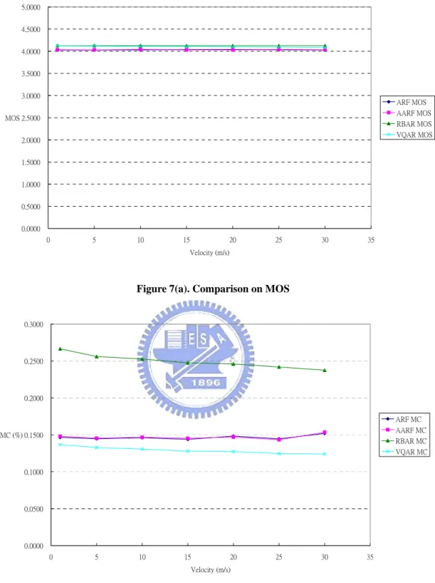
4.2.2 Moving MS at different Velocity

In the second scene, we let the MS move in a fixed velocity from 1m/s up to 30m/s. The MS starts at 50m away from the BS and moves away from the BS until it reaches 200m. Then the MS moves back toward the BS until it reaches 50 m away from the BS. This back and forth movement is done for 10 times, the results of this simulation are shown in Figure 7.

As we can see in Figure 7(a), MOS value of VQAR , ARF/AARF and RBAR are roughly the same just above four. Their difference, again, isn’t significance for human ear, since the MOS values are all slightly above four.

The MC values are shown in Figure 7(b). As we could see, VQAR maintains a lower MC than RBAR and ARF/AARF. The MC of ARF/AARF seem to grow with velocity is because ARF/AARF has a slower reaction to mobility. RBAR and VQAR could response faster since rate selection is based on the SNR value. RBAR is higher than VQAR by the same reason mentioned in 4.2.1, it drops rates faster than needed.

(21)

15 0.0000 0.5000 1.0000 1.5000 2.0000 2.5000 3.0000 3.5000 4.0000 4.5000 5.0000 0 5 10 15 20 25 30 35 Velocity (m/s) MOS ARF MOS AARF MOS RBAR MOS VQAR MOS

Figure 7(a). Comparison on MOS

0.0000 0.0500 0.1000 0.1500 0.2000 0.2500 0.3000 0 5 10 15 20 25 30 35 Velocity (m/s) MC (%) ARF MC AARF MC RBAR MC VQAR MC Figure 7(b). Comparison on MC

(22)

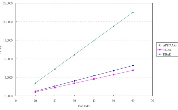
16 4.2.3 Multiple MS nodes comparison

In the third scene, we increase the amount of MS nodes connected to the BS nodes from 10 nodes to 60 nodes. All nodes are set at a fixed distance 150m away from the BS. The simulation results of MOS and MC values are shown in Figure 8.

In Figure 8(a), we could see that the MOS values are roughly the same for all four algorithms. Although VQAR is slightly better than the other three algorithms, as mentioned before, this difference is not significance for human ear, since the MOS values are all slightly above four. The MC values are shown in Figure 8(b). VQAR has the lowest MC out of the four algorithms as we expected, ARF/AARF slightly higher and RBAR at the highest. This order maintains as we increase the amount of MS nodes. From Figure 8(c), we examine the MC value of a single MS node. Compared with Figure 6(b), the MC value of a single is slightly larger in the multi MS node scene, due to the fact more collisions occur when the more MS nodes exists. The MC value of ARF/AARF is about 1.18 time higher than VQAR, and RBAR is about 2.75 times higher. This difference is also the same when we count summation MC of all MS nodes in Figure 8(b).

0.0000 0.5000 1.0000 1.5000 2.0000 2.5000 3.0000 3.5000 4.0000 4.5000 5.0000 0 10 20 30 40 50 60 70 # of nodes MOS ARF/AARF VQAR RBAR

(23)

17 0.0000 5.0000 10.0000 15.0000 20.0000 25.0000 0 10 20 30 40 50 60 70 # of nodes MC ( % ) ARF/AARF VQAR RBAR

Figure 8(b). Comparison on MC (summation of all MS nodes)

0.0000 0.0500 0.1000 0.1500 0.2000 0.2500 0.3000 0.3500 0.4000 0.4500 0 10 20 30 40 50 60 70 # of nodes MC (%) ARF/AARF VQAR RBAR

Figure 8(c). Comparison on MC (of single MS node)

Figure 8. Different Algorithm’s MOS & MC with different amount of MS nodes.

Some may wonder the effectiveness of VQAR in real environment when multiple MS nodes exist. When more nodes exist, MC would increase due to failure transmission from congestion. However, this increase would affect all rates. And like PLC, when transmission failure is due to congestion, we should intend to maintain current transmission rate instead of

(24)

18

lowering to prevent further collisions. Increasing transmission rate wouldn’t be suitable since the medium condition isn’t suitable for a higher transmission rate. So if VQAR selects rate on a predetermined MC chart might not guarantee the selected rate to have the same MC in multiple MS node situation, it still can guarantee that the selected rate tends to have the lowest MC than other rates.

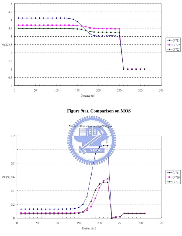
4.3 Codec Influence

Besides the tests and comparison ran in our simulation, there are further simulations to run. As shown in Figure 9 we could expand determination of sustainable rate to be by SNR and also by codec. We simulate traffic of G.711, G.723, and G.729 codec, their bit rates are 64kb/s, 5.6kb/s, and 8kb/s. Although these codec’s sampling rate are all 8kHz, they differ in the bit rate after coding.

From Figure 9(a) we could see that G.711 with the highest bit rate has the highest MOS value at the beginning but drop lower than 3.5 MOS around 170m. The drop is due to the high amount of data G.711 used for coding so when error starts to occur, G.711 lost more data than the lower bit rate codec. G.723 and G.729 suffer from the same effect, but slighter than G.711. Because G.723 uses the smallest bit rate, it has the highest distortion after coding resulting in a low MOS value. And in Figure 9(b) we could see that the MC value with G.711 highest, following G.729 and G.723 at the lowest, in the order of their bit rate.

(25)

19 MOS of Different Codec (Rt=24Mbps)

0 0.5 1 1.5 2 2.5 3 3.5 4 4.5 5 0 50 100 150 200 250 300 350 Distance (m) MOS G.711 G.729 G.723

Figure 9(a). Comparison on MOS

MC of Different Codec (Rt=24Mbps) 0 0.2 0.4 0.6 0.8 1 1.2 0 50 100 150 200 250 300 350 Distance(m) MC(%) G.711 G.729 G.723 Figure 9(b). Comparison on MC

(26)

20

Chapter 5 Conclusion and Future Work

When transmitting VoIP traffic over wireless medium under mobility conditions, using the same rate for transmission would not be suitable. Rates too fast would result in massive packet loss; rates too slow would result in high occupation of a single station. Our problem statement is to find and choose a most efficient sustainable rate which guarantees certain quality and maximum utilization for VoWLAN transmission under mobile movements. We

use MOS and MC for quality and utilization evaluation, so we would select a rate Rs(SNR)

that satisfies MOS > 3.5 with minimum MC for transmission rate. The mapping of Rs(SNR)

can be calculated by observing the MOS and MC value of all rates under all possible medium conditions, then selecting the rate satisfying our criteria.

From the simulation result previously, we could see that VQAR, ARF/AARF and RBAR all guarantee a suitable quality (MOS > 3.5) for voice transmission under static MS with different distance to BS, moving MS at different velocity, and multiple MS nodes. But VQAR has a lower MC than ARF/AARF and RBAR in most situations. Averagely speaking, MC value of VQAR is 11% lower than ARF/AARF and 27% lower than RBAR. Such difference is even more obvious in multiple MS nodes. VQAR not only guarantee a satisfying quality for VoIP traffic, but also guarantee a better medium utilization than other algorithms. Transmission quality and high utilization are both satisfied when we use VQAR for rate adaptation.

Further work could be done by letting rate selection of VQAR also based on different codec, since MOS and MC behavior also differs under different codec as shown in 4.3.

(27)

21

References

[1] William Stallings, “Wireless Communications and Networks,” Prentice Hall, pp. 100-160, 2002.

[2] “Telephone transmission quality subjective opinion tests. A method for subjective performance assessment of the quality of speech voice output devices,” ITU-T Recommendation, pp. 85, 1994.

[3] The Network Simulator – ns-2, <http://www.isi.edu/nsnam/ns/>

[4] M. Lacage, M. H. Manshaei, and T. Turletti, “IEEE 802.11 Rate Adaptation: A Practical Approach,” IEEE MSWiM’04, October 2004.

[5] C. W. Huang, A. Chindapol, J. A. Ritcey, and J. N. Hwang, “Link Layer Packet Loss Classification for Link Adaptation in WLAN,” Information Sciences and Systems, 2006 40th Annual Conference, pp.603-608.

[6] S. Pal, S. R. Kundu, K.Basu, and S. K. Das, “IEEE 802.11 Rate Control Algorithms: Experimentation and Performance Evaluation in Infrastructure Mode,” In PAM '06, 2006.

[7] Gavin Holland, Nitin Vaidya, and Parmvir Bahl, “A Rate-Adaptive MAC Protocol for Multi-Hop Wireless Network,” ACM SIGMOBILE, 2001

[8] J. Matta, C. Pepin, K. Lashkari, and R. Jain, “A Source and Channel Rate Adaptation Algorithm for AMR in VoIP Using the Emodel,” NOSSDAV, pp. 92-99, Monterey, USA, Jun 2003.

[9] T. Branskich, N. Smavatkul, and S. Emeott, “Optimization of a Link Adaptation Algorithm for Voice over Wireless LAN Application,” IEEE Communications, 2005. [10] A. Trad, Q. Ni, and H. Afifi, “Adaptive VoIP Transmission over Heterogeneous

Wired/Wireless Networks,” MIPS 2004, Grenoble, France, November 17-19, 2004. [11] M. Bandinelli, F. Chiti, R. Fantacci, D. Tarchi, G. Vannuccini, “A Link Adaptation

strategy for QoS support in IEEE 802.11e-based WLANs,” IEEE Communications, 2005 [12] Z. Qiao, L. Sun, N. Heilemann, and E. Ifeachor, “A new method for VoIP Quality of

Service Control use combined adaptive sender rate and priority marking,” IEEE Communications, 2004