Optimal design of panel speaker array with omnidirectional characteristics

Optimal design of panel speaker array with omnidirectional

characteristics

Mingsian R. Baia)and Kuochan Chung

Department of Mechanical Engineering, National Chiao-Tung University, 1001 Ta-Hsueh Road, Hsin-Chu 300, Taiwan, Republic of China

共Received 31 August 2001; accepted for publication 31 July 2002兲

A panel speaker system intended for a projection screen is developed. Like other sound sources with large dimension, the panel speaker has a beaming problem in high frequencies. To alleviate the problem, panel speakers are integrated into an array, with optimal electronic compensation for omnidirectional response and array efficiency. The heart of the design procedure is a three-stage optimization scheme involving two nonlinear and nonconvex objectives. The process is interactive, allowing the array coefficients to be tailored so that the specifications of directional response can be met. The optimal design of panel speaker array is then implemented by using a multichannel digital signal processor. In addition, a Hilbert transformer is required to produce the quadrature components of the array coefficients. A small array and a large matrix were constructed to validate the implemented array signal processing system. The experimental results indicate that, without degradation of efficiency, the proposed optimization technique in conjunction with electronic compensation is effective in attaining omnidirectional radiation property. © 2002 Acoustical

Society of America. 关DOI: 10.1121/1.1509435兴

PACS numbers: 43.38.Ar 关SLE兴

I. INTRODUCTION

This work focuses on the development of a projection screen which is composed of panel speakers. This system is intended for applications such as oral presentation, public addressing, or home theater. The system integrates both the audio and video functions into one unit, which may provide certain advantages over conventional systems. The main rea-son for using panel speakers lies in the flatness and compact-ness, which makes them well suited for the application as a projection screen. In general, a large and properly designed panel speaker is less directional in high frequencies than con-ventional cone speakers. However, a detailed electroacoustic analysis1 revealed that this desirable property of panel speaker comes at the expense of efficiency. Furthermore, like other sound sources with large dimension, the panel speaker will still suffer from a peculiar beaming problem at coinci-dence angles in high frequencies if the radiating area is large.2As a solution to the above problem, this paper pre-sents a speaker array approach, using an idea that contradicts the original distributed mode concept of panel speakers. We use small panels which are as light and stiff as possible to produce coherent but directional sound beams. Then, using electronic compensation and digital signal processing, we seek to achieve simultaneously omnidirectional response and array efficiency. If individual elements are identical, then the proposed beamforming technique also is applicable to arrays of conventional loudspeakers. The analysis and design of conventional loudspeaker arrays can be found in the literature.3– 6 It is also pointed out by the reviewer that a sound and light spectacle in Mexico used an array of panel speakers as the projection screen. This technology, invented

by Sound Advance, is similar to a conventional cone speaker in as much as it uses a voice coil assembly.7However, it uses a flat diaphragm molded from expanded polystyrene, which allows the user to flush mount it inside a wall or ceiling in ‘‘invisible’’ fashion.

The design of an omnidirectional array boils down to finding a set of array coefficients that gives rise to a ‘‘flat spectrum’’ in the wave number space. For a linear array with real coefficients, direct inversion of an all-pass flat spectrum will apparently lead to the trivial solution: only one single element is active at the origin. This case corresponds to an array with very poor efficiency. Hence, two approaches have been proposed to avoid running into the dilemma between flat spectrum and array efficiency. One approach is to intro-duce a phase function into the directional response. The Bessel array and the quadratic phase array共QPA兲 are based on this idea.6 The array gains in the QPA are purely phase compensation in quadratic forms. Another approach8 is to choose a white-noise-like sequence with low correlation property, e.g., the Barker code, the Huffman code, and the maximum flatness sequence to produce a flat spectrum of array radiation pattern.

Different from the earlier approaches, an optimization technique is proposed in this paper to find array coefficients that maximize two cost functions: flatness and efficiency. This problem turns out to be a nonlinear and nonconvex problem for which it is generally very difficult to locate the global optimum. Hence, instead of finding the global opti-mum, we are content with the solution of a three-stage sub-optimal problem. The design process is interactive, allowing us to tailor the array coefficients so that the specifications of directional response can be met. The array coefficients thus found are generally complex numbers, which entail the implementation of a Hilbert transformer.9–11 The Hilbert a兲_{Electronic mail: msbai@cc.nctu.edu.tw}

transformer can be implemented in either IIR or FIR filter;9 we will only discuss the latter approach.

A 5⫻1 panel speaker array and a 3⫻3 panel speaker array were constructed for experimental verification. Signal processing and electronic compensation are carried out by using a multichannel digital signal processor共DSP兲. Results will be compared and discussed with regard to an uncompen-sated array and the array obtained using the proposed opti-mization technique.

II. FAR-FIELD MODEL FOR UNIFORM LINEAR ARRAYS

A panel speaker array is schematically shown in Fig. 1共a兲. Audio signals are processed, often digitally, by a bank of filters before feeding to the power amplifiers and panel speakers. With reference to the geometry of Fig. 1共b兲, the far-field pressure radiated by a source array with 2N⫹1 equally spaced elements can be expressed as6,12

P共r,␪, f兲⫽A共 f ,␪兲R共 f ,r兲B共 f ,␪兲, 共1兲

where d is the spacing between two adjacent speakers, r Ⰷd is the distance between the array center and a far-field observation point,␪ is the angle measured from the normal to the array, f is the frequency, c is the sound speed, A( f ,␪) is the radiation pattern of each source, R( f ,r)

⫽r⫺1_{exp(j2␲fr/c) represents the spherical spreading,} B( f ,␪) is the array pattern, defined as

B共 f ,␪兲⫽

兺

N

g_n共 f 兲ej共2␲n f d sin␪/c兲, 共2兲 with gn( f ) being the array coefficient of the nth element.

Using the array filters, one is able to manipulate the array pattern to obtain the desired directional response.

Hereafter, we further restrict the array coefficients gn( f )

to be frequency-independent, complex constants, gn. The

array pattern can then be written as

B共u兲⫽

兺

N

gnejnu, 共3兲

where u⫽2␲f d sin␪/c is a dimensionless angle. Inspection of Eq. 共3兲 reveals that the array pattern is essentially the frequency response of an FIR filter with coefficients g_n. That is, the design problem of an omnidirectional array can be regarded as the design of an FIR all-pass filter. For latter use, define the angular spectrum

S共u兲⫽储B共u兲储₂2, 共4兲

where储 储2 denotes the 2-norm, and the autocorrelation

R共k兲⫽

兺

⬁

gngk*_⫺n, 共5兲

where k is the array index, gn has a compact support within

关⫺N,N兴, ‘‘*’’ denotes complex conjugate. It can be shown that the angular spectrum is the Fourier transform of the autocorrelation, i.e.,

S共u兲⫽

兺

N

R共k兲e⫺ jku. 共6兲

III. OBJECTIVES AND CONSTRAINTS

As mentioned earlier, the design goal of our problem is to find an array with omnidirectional characteristics and good efficiency. In this section, these design objectives will be formulated as two performance indices: spectral flatness and array efficiency.

A. Array efficiency

The array efficiency of a (2N⫹1)⫻1 array is defined as ␩⫽_{共2N⫹1兲兩g兩}R共0兲

⬁, 共7兲

where g⫽兵gn兩⫺N⭐n⭐N,n苸N其, 兩g兩⬁⫽max兵gn兩⫺N⭐n

⭐N其is the infinity norm of g, and

R共0兲⫽

兺

冕

where the Parseval theorem has been invoked. Array effi-ciency is thus the mean-squared array gains normalized by 兩g兩_⬁. The physical meaning of the array efficiency can be interpreted as the degree of participation of active array ele-ments. The efficiency will be close to unity if most array elements are active with full power共large gain values gn). FIG. 1. A uniform linear array.共a兲 The schematic of a panel speaker array;

B. Spectral flatness

For the same array, the merit factor, or the spectral flat-ness, is defined as12,13

F⫽ R

2_共0兲 兺k⫽0兩R共k兲兩2

. 共9兲

Using Eq.共6兲, we have 1 2␲

冕

冕

兺

According to the Parseval’s relation, we have

兺

冕

Substituting Eqs.共10兲 and 共11兲 into Eq. 共9兲 gives

F⫽ 共兰⫺␲

␲ _{S共u兲du兲}2

2␲兰_⫺␲␲ 关S2_共u兲⫺R2_共0兲兴du. 共12兲

The denominator of F can also be written as

冕

冕

⫺␲ ␲

关S共u兲⫺R共0兲兴2_{du. 共13兲} From Eqs.共12兲 and 共13兲, the spectral flatness F is the ratio of the mean-square spectrum over the spectral variance. An ar-ray with omnidirectional response tends to have large spec-tral flatness.

C. Constraints

Unfortunately, the aforementioned objective functions are not sufficient to reach a unique solution because any array coefficients differing within a scaling and/or a rotation will lead to identical F and␩. This fact will be detailed in the following analysis.

Let C and R be the sets of real numbers and imaginary numbers, respectively. Suppose an array coefficient set g1 can be obtained from another set g⫽兵gn兩⫺N⭐n⭐N其 by a

magnitude scaling r and a finite rotation u0, i.e.,

g1⫽T共r,u0,g兲⫽兵rgne⫺ jn␦兩⫺N⭐n⭐N,r苸C,u0苸R其.

共14兲 Then, it is not difficult to verify the spectrum of the new coefficients

S1共u兲⫽兩r兩2_{S共u⫹u0兲. 共15兲}

The spectrum is scaled by a factor兩r兩2_{and shifted in u axis} by u₀. Furthermore, the spectral flatness and array efficiency remain invariant under the transformation T(r,u₀,g), i.e.,

F1⫽F, ␩1⫽␩, 共16兲

and both coefficient sets are considered ‘‘equivalent.’’ Con-sequently, additional constraints are needed to resolve this nonuniqueness problem. These constraints are derived from the following theorem. Theorem: For a (2N⫹1)⫻1 array, consider an array coefficient set g⫽兵gn兩⫺N⭐n⭐N其, with

兩g兩_⬁⫽兩g0兩. 共17兲

Using the equivalent transformation of Eq. 共14兲, the array coefficient set g can always be transformed into a ‘‘reduced’’ array coefficient set J given by

J⫽兵J_n兩J_n苸C, 兩J_n兩⭐1, ⫺N⭐n⭐N, J0⫽1 and ⬔J0⫽⬔J1⫽0其 共18兲 Proof: Let r0⫽e⫺ j⬔g0_/兩g兩 ⬁, ␦0⫽⬔g0⫺⬔g1, and J⫽T共r0,␦0,g兲 ⫽

再

冎

Substituting Eq. 共17兲 into 共19兲 leads to: J0⫽1, J1 ⫽兩g1/g0兩, and 兩J兩⫽兩gn/g0兩⭐1. Hence,

J⫽兵Jn兩Jn苸C, 兩Jn兩⭐1, ⫺N⭐n⭐N, J0⫽1 and

⬔J0⫽⬔J1⫽0其,

which is Eq.共18兲. Q.E.D.

Thus, on the basis of the theorem, the feasible solution set of the array design problem can be dramatically reduced by imposing the following ‘‘fundamental constraints’’ in optimi-zation:

g0⫽1, ⬔g0⫽⬔g1⫽0 and 兩gn兩⭐1, ⫺N⭐n⭐N. 共20兲

Under this constraint, the maximum magnitude of array gain never exceeds unity.

IV. THE THREE-STAGE OPTIMIZATION PROCEDURE In this section, an optimization technique is proposed to find array coefficients that maximize the aforementioned two cost functions: flatness and efficiency. Unfortunately, this problem turns out to be a nonlinear, nonconvex, and multi-objective problem for which it is generally very difficult and time-consuming to locate the global optimum. Hence, in-stead of finding the global optimum, we seek to find a sub-optimal solution by using a three-stage optimization scheme—two stages for single-objective optimization and one stage for weighting two objectives.

A. The first stage: Phase optimization

To reiterate, the goal for the array design is to find array coefficients with high array efficiency and flat spectrum. For high efficiency, the magnitude of each array coefficient should be close to unity. For flat spectrum, the array coeffi-cient set should be a random sequence with low correlation property. Putting these two statements together, one may conclude that the desired array coefficient set should be a random sequence satisfying two conditions: 兩gn兩⬇1 and

⬔gnis a random number over关0,2␲兴. Thus, in the first stage

of optimization, we restrict the magnitude of each array co-efficient at a ‘‘full efficiency’’ state, i.e., 兩gn兩⫽1, and adapt

the phases as randomly as possible. The optimization prob-lem in this stage can be stated as

Max ␪k苸R,⫺N⭐k⭐N F⫽ R 2_共0兲 兺k_⫽0R2共k兲 , 共21兲

subject to the aforementioned fundamental constraints, and the ‘‘full efficiency constraint,’’ defined as

兩gk兩⫽1, ⫺N⭐k⭐N. 共22兲

In this setting, the optimization in the first stage has only a single objective, spectral flatness. The constrained steepest

descent共CSD兲14method is employed to find the local maxi-mum, or the ‘‘full efficiency point.’’

However, the result of the search is quite sensitive to initial conditions because the problem is nonlinear and non-convex. As motivated by the characteristics of the optimal array, we thus adopted a heuristic but efficient approach and assigned random numbers to the phases as the initial guess. A simulation result obtained using the first-stage optimization for a 13⫻1 array is shown in Fig. 2. This simulation took approximately 1 min on a personal computer. The result was found by performing the first-stage optimization 20 times and selecting the flattest pattern as the full efficiency point. The step size of optimal search starts at 0.3 and decreases for convergence. Each optimization converged within 100 itera-tions. The calculated array coefficients are listed in Table I. It can be seen from the result that the angular spectrum fluctu-ates randomly since spectral flatness is not optimized in this stage.

B. The second stage: Magnitude and phase optimization

In this stage, both magnitude and phase of array coeffi-cients are adjusted to further improve spectral flatness. After phase adapting, the only way to obtain more flatness is to adjust the magnitude of array coefficients. In effect, such optimization procedure is a ‘‘tapering’’ process of magnitude to get a broader and flatter spectrum, at the cost of array efficiency. The optimal problem in this stage is formulated as follows: Max ␪k苸R,⫺N⭐k⭐N F⫽ R 2_共0兲 兺k⫽0R2共k兲 , 共23兲

subject to the fundamental constraints. The initial guess is the full efficiency point found in the last stage. The optimi-zation in this stage is a nonlinear and nonconvex problem with one objective, flatness. CSD is used to find the subop-timal solution that is called the ‘‘flattest point.’’

The example of the 13⫻1 array is used again for the second-stage optimization. The result corresponding to the flattest point is also shown in Fig. 2. The array coefficients are listed in Table I. If the status of each iteration in this optimization stage is recorded, a trade-off can be observed between the flatness and efficiency. The search path for the 13⫻1 array is shown in Fig. 3. It can be seen in the plot that flatness is a monotonically increasing function of efficiency. The curve is terminated at both ends by the flattest point and the full efficiency point, respectively. The search path is

FIG. 2. The angular spectra at the full efficiency point and the flattest point for the 13⫻1 optimal array.

TABLE I. The array coefficients for the 13⫻1 optimal array at 共a兲 the full efficiency point and共b兲 the flattest point.

Array index 共a兲 共b兲

⫺6 exp(j0.06) 0.21 exp(⫺j1.27) ⫺5 exp(⫺j1.05) 0.51 exp(⫺j2.10) ⫺4 exp(⫺j1.81) 0.58 exp(⫺j2.10) ⫺3 exp(⫺j0.63) 0.72 exp(⫺j1.67) ⫺2 exp(⫺j1.41) 1.00 exp(⫺j2.40) ⫺1 exp(j3.07) 0.76 exp(j3.13) 0 1 1 1 1 0.76 2 exp(j1.43) 1.00 exp(j2.40) 3 exp(⫺j2.55) 0.73 exp(⫺j1.48) 4 exp(j1.78) 0.58 exp(j2.08) 5 exp(⫺j2.05) 0.50 exp(⫺j1.05) 6 exp(⫺j0.10) 0.21 exp(j1.25) Flatness 18.74 360 Efficiency 1 0.50

FIG. 3. The search path of efficiency and flatness for the 13⫻1 optimal array.

stored in the computer for final tuning of the efficiency and flatness.

C. The third stage: Tuning of efficiency and flatness As shown in Fig. 3, the search path for the array lies within the window

0.50⭐␩⭐1, 共24兲

and

19.68⭐F⭐360, 共25兲

which renders the reachable performance limit in the design. In the third stage, the following template is employed as the desired spectrum:

Sd共u兲⫽Rd共0兲⫹Aripplesin u/T, 共26兲

where Rd(0) and Aripplerepresent, respectively, the mean and the ripple size of the desired spectrum. For example, let

Rd(0)/Aripple⫽10. Substituting Eq. 共26兲 into Eq. 共12兲, the

corresponding flatness should be

Fd⫽2共Rd/Aripple兲2⫽200. 共27兲

Using the search path in Fig. 3, one can find the correspond-ing efficiency to be 0.56. Recall the definition of array effi-ciency

␩⫽Rd

2_{共0兲/2N⫹1⫽0.56, 共28兲}

where N⫽6 for a 13⫻1 array. Solving Eqs. 共27兲 and 共28兲 yields Rd(0)⫽7.30 and Aripple⫽0.73, based on which the

desired spectrum is given by

Sd共u兲⫽7.28⫹0.728 sin u

T. 共29兲

If the result is acceptable, the corresponding array coeffi-cients will be retrieved from the computer and the actual spectrum will be calculated. Otherwise, one should select another Rd(0)/Arippleand repeat this optimization stage. The desired spectrum and the actual spectrum for the example are compared in Fig. 4. Two spectra have similar ripple size and

spectrum mean. The flow chart of the optimization with three stages is shown in Fig. 5.

D. QPA array versus the optimal array

To justify the proposed technique, the 13⫻1 array de-signed using our optimization method is compared to the QPA array (z⫽18) where z is the shape factor. The array gains in the QPA are purely phase compensation in quadratic forms, z(1⫺兩␪兩/␲)␪/␲. The details of the QPA array can be found in Ref. 6. The array coefficients used in this simulation are listed in Table II. The angular spectra in Fig. 6 show that the spectrum of our array appears flatter than that of the QPA array. This is also reflected in Table II, where the calculated flatness is 11.5 vs 114.9 for the QPA array and our array, respectively, with identical efficiency.

V. EXPERIMENTAL INVESTIGATIONS

Two panel speaker arrays are constructed for experimen-tal verification of the proposed array signal-processing tech-niques. In this section, a technical, but critical, issue in

FIG. 4. The desired spectrum vs calculated spectrum for the 13⫻1 optimal array (F⫽200) found in the third stage.

implementing complex array coefficients shall be addressed, followed by hardware implementation of a 5⫻1 small array and 3⫻3 large array.

A. The implementation of complex array coefficients As noted earlier, the resulting array coefficients gn

ob-tained using the proposed optimization techniques are gener-ally complex. Although they are constants in nature, the ap-proximation of which calls for the use of frequency-dependent filters

gn共␻兲⬇Re兵gn其⫹ j Im兵gn其, 共30兲

where␻is the digital frequency, n is the array index, and j ⫽

冑

and output bn is given as

A共ej␻兲⫽关Re兵gn其⫹H共ej␻兲Im兵gn其兴B共ej␻兲, 共31兲

where A(ej␻) and B(ej␻) are discrete Fourier transforms of

an and bn, respectively. The Hilbert transformer9 H(ej␻)

serves to generate a quadrature component. The frequency response of an ideal Hilbert transformer is

H共ej␻兲⫽

再

0⭐␻⭐␲

j, ⫺␲⭐␻⬍0, 共32兲

and the associated impulse response h关n兴 is

h关n兴⫽

再

Ha共ej␻兲⫽

再

e⫺ j共M␻⫹␲/2兲, 0⭐␻⭐␲

e⫺ j共M␻⫺␲/2兲, ⫺␲⭐␻⬍0. 共34兲 The frequency response of the modified array filter then be-comes

gn共␻兲⬇e⫺ jM␻兵Re兵gn其⫹ j Im兵gn其其⫽e⫺ jM␻gn. 共35兲

Note that no waveform distortion will arise due to the pure delay. Figure 7共b兲 shows the implementation in more detail. Using the implementation shown in Fig. 7共b兲 and substitut-ing Eq. 共35兲 into 共2兲, we have

B共␪,␻兲⫽e⫺ jM␻

兺

where f⫽ fs␻/2␲, fs is the sampling frequency, f is analog

frequency, and ␻is digital frequency. Hence, the system in Fig. 7共b兲 yields an array pattern with the same magnitude response as the desired pattern. The Hilbert transformer

TABLE II. The comparison of 13⫻1 QPA (z⫽18) and the 13⫻1 optimal array when the optimal array and QPA has the same efficiency.

Array index QPA (z⫽18) Optimal array

⫺6 0.74 0.35 exp(⫺j0.78) ⫺5 ⫺0.78 0.61 exp(⫺j1.78) ⫺4 0.96 0.66 exp(⫺j1.92) ⫺3 ⫺1.00 0.90 exp(⫺j1.22) ⫺2 0.45 1.00 exp(⫺j2.09) ⫺1 0.67 0.90 exp(j3.09) 0 ⫺0.86 1 1 ⫺0.67 0.94 2 0.45 1.00 exp(j2.03) 3 1.00 0.88 exp(⫺j2.02) 4 0.96 0.62 exp(j1.79) 5 0.78 0.59 exp(⫺j1.52) 6 0.74 0.37 exp(j0.57) Flatness 11.53 114.9 Efficiency 0.63 0.63

FIG. 6. The spectra of the QPA (z⫽18) and the optimal array 共13⫻1兲, where both arrays have equal efficiency.

FIG. 7. The implementation diagram of complex array coefficients. 共a兲 Single-channel array filter and the Hilbert transformer; 共b兲 multichannel implementation.

can be implemented by either an FIR9 filter or an IIR10,11 filter. In this work, we chose to use the FIR implementation. The Kaiser window approximation for a Hilbert transformer of order M takes the form9

h关n兴⫽

冦

再

冎

will introduce frequency-dependent delay and result in some waveform distortion.

B. The experimental result of a 5Ã1 linear panel speaker array

Although the ultimate goal of this work was to develop the large panel speaker array, we use a small array to verify the far-field behavior because of the limitation of current measuring environment. A 5⫻1 panel speaker array is con-structed for experimental verification. The system consists of using PU-foam panel speakers, array signal-processing unit, a monitoring microphone, data acquisition unit, and a step-ping motor unit. The dimensions and structure of the 5⫻1 panel speakers are shown in Figs. 8共a兲 and 共b兲. The size of each rectangular panel is 7⫻6.7 cm2 and the spacing be-tween adjacent speakers, d⫽6.7 cm. Each panel is driven by an electromagnetic exciter mounted on an aluminum frame. The photo of the array hardware is shown in Fig. 8共c兲.

The array signal processing is carried out by a floating-point DSP, TSM320C32 in conjunction with a multiple-channel IO module. Audio signals are fed to the array signal-processing unit, through AD conversion and power

amplifi-FIG. 8. The small panel speaker array.共a兲 Configuration of the 5⫻1 panel speaker array;共b兲 dimensions of panel speakers and the location of exciter;

cation, and generate compensated signals for each channel of speaker. The monitoring microphone is situated 2 m from the center line of the array. The array is mounted on a turntable driven by the stepping motor so that directional responses of the array within关⫺90°, 90°兴 can be recorded automatically, with every 1° increment. Necessary data acquisition/ processing and motor control are all handled by the DSP as well. The experiments are conducted inside an anechoic chamber.

An experiment was conducted to compare the optimal panel speaker array to an uncompensated array (gn

⫽1,᭙n). The optimal set of coefficients of the 5⫻1 array was found using the proposed optimization technique

gopt⫽兵⫺0.45,j,1,j,⫺0.45其. 共38兲

The Hilbert transformer was implemented by a 100-tap FIR filter with a 50-sample delay, and sampling rate is 20 kHz. The directional response of the panel speaker array is mea-sured at 2 and 3 kHz, respectively, on the horizontal plane of the array. Drastic differences can be observed in the experi-mental results of Fig. 9. The array is indicated in the figure. The uncompensated array indeed radiates a rather directional

pattern, whereas the optimal array exhibits a relatively om-nidirectional behavior.

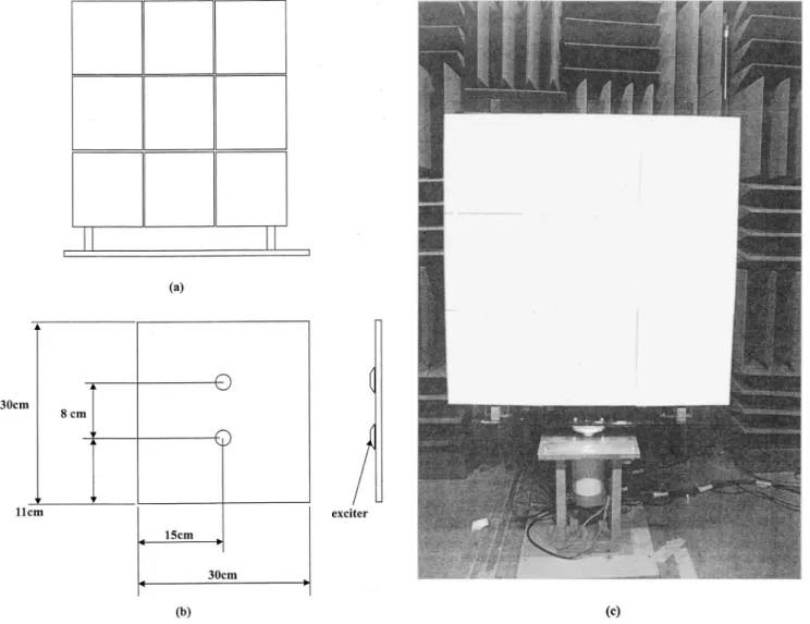
C. The experimental result of a 3Ã3 panel speaker matrix

To further justify the panel speaker array, a large 3⫻3 matrix of the size of a projection screen is constructed using PU-foam panels, covered with glassy face skins. The dimen-sions and structure of the 3⫻3 panel speakers are shown in Fig. 10共a兲. The size of each panel is 30⫻30 cm2 and the spacing between adjacent speakers, d⫽30 cm. The photo of the array hardware is shown in Fig. 10共b兲. Despite the matrix configuration, the array is based on one-dimensional com-pensation in the horizontal direction, which in our applica-tion is considered more important than the vertical direcapplica-tion. Each panel is driven by two electromagnetic exciters mounted on an aluminum frame. The three panels at each column are wired together to the same DSP output and six exciters are all in parallel connection. The rest of the details of experimental arrangement are identical to those of the 5⫻1 array.

An experiment was conducted to compare the optimal panel speaker array to an uncompensated array. The optimal

FIG. 10. The large panel speaker array of a projection screen.共a兲 Configuration of the 3⫻3 panel speaker array; 共b兲 dimensions of panel speaker and the location of the exciter;共c兲 The photo of the 3⫻3 panel speaker array of a projection screen.

set of coefficients of the 3⫻3 array was found using the proposed optimization technique

gopt⫽兵⫺0.45j,1,⫺045j其. 共39兲

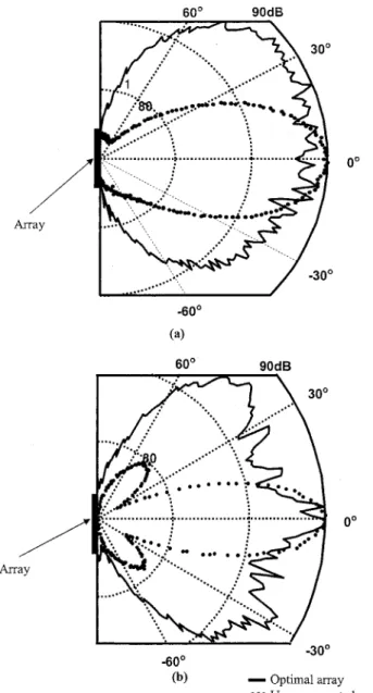
The Hilbert transformer was implemented by a 150-tap FIR filter with a 75-sample delay, and sampling rate is 10 kHz. The directional responses of the panel speaker array is mea-sured at 488 and 780 Hz, respectively, on the horizontal plane of the array. It is noted that in this large array experi-ment, we were able to investigate only near-field radiation pattern in our anechoic room. Similar to the case of small array, drastic difference can be observed in the experimental results of Fig. 11. The uncompensated array radiates a quite directive pattern, whereas the optimal array exhibits a rela-tively omnidirectional behavior.

VI. CONCLUSIONS

An important feature of this paper is the array optimiza-tion method, and the projecoptimiza-tion screen is a practical example

of its use. Electronic compensation is employed to achieve omnidirectional response and array efficiency. Optimal de-sign of array coefficients is computed by a three-stage opti-mization procedure that effectively solves the nonlinear and nonconvex problem. The process is interactive, allowing us to tailor the array coefficients to meet the design specifica-tions. The array design obtained using the optimization tech-nique has been implemented by using a multichannel DSP, where a Hilbert transformer is required to produce the quadrature components of the array coefficients. A small ar-ray and a large matrix were constructed to validate the imple-mented array signal-processing system. The experimental re-sults obtained from the DSP-based system indicate that the optimally compensated panel speaker array exhibits omnidi-rectional radiation pattern without degradation of efficiency. With regard to the use of panel speakers as projection screens, there are a few technical points to consider. These include the added brightness that can be achieved with a nonperforated screen, as well as the degree to which the response of large speaker arrays suffers from time smearing and poor stereo imaging.

Although the ultimate goal of this work was to develop the large array, we were unable to verify its far-field behavior due to the limitation of current measuring environment. Much work is continuing in improving the implementation as well as measurement of the large array for future research. ACKNOWLEDGMENTS

Special thanks are due to the illuminating discussions with NXT, New Transducers Limited, UK. The work was supported by the National Science Council in Taiwan,

Re-public of China, under the project number NSC

89AFA06000714.

1_{M. R. Bai and T. Huang, ‘‘Development of Panel Loudspeaker System:}

Design, Evaluation and Enhancement,’’ J. Acoust. Soc. Am. 109, 2751– 2761共2001兲.

2

L. E. Kinsler, A. R. Ffrey, A. B. Coppens, and J. V. Sanders, Fundamentals

of Acoustics共Wiley, New York, 1982兲.

3_{D. L. Smith, ‘‘Discrete-Element Line Arrays—Their Modeling and}

Opti-mization,’’ J. Audio Eng. Soc. 45, 949–964共1997兲.

4

G. L. Augspurger, ‘‘Near-Field and Far-Field Performance of Large Woofer Arrays,’’ J. Audio Eng. Soc. 38, 231–236共1990兲.

5_{D. G. Meyer, ‘‘Digital Control of Loudspeaker Array Directivity,’’ J.}

Au-dio Eng. Soc. 32, 747–754共1984兲.

6_{R. M. Aarts and A. J. E. M. Janssen, ‘‘On Analytic Design of Loudspeaker}

Arrays with Uniform Radiation Characteristics,’’ J. Acoust. Soc. Am. 107, 287–292共2000兲.

7_{Sound Advance, http://soundadvance.com/.}

8_{G. F. M. Beenker, T. A. C. M. Claasen, and P. W. C. Hermens, ‘‘Binary}

Sequences with a Maximally Flat Amplitude Spectrum,’’ Philips J. Res.

40, 289–304共1985兲.

9_{A. V. Oppenheim and R. W. Schafer, Discrete-Time Signal Processing}

共Prentice-Hall, Englewood Cliffs, NJ, 1989兲.

10_{Z. G. Jing, ‘‘A New Method for Digital All-Pass Filter Design,’’ IEEE}

Trans. Acoust., Speech, Signal Process. 35, 1557–1564共1987兲.

11_{B. Gold, A. V. Oppenheim, and C. M. Radar, ‘‘Theory and Implementation}

of the Discrete Hilbert Transformer,’’ in Proc. Symp. Computer Processing

in Communications, Vol. 19共Polytechnic, New York, 1970兲.

12

D. F. Johnson and D. F. Dudgeon, Array Signal Processing Concepts and

Techniques共Prentice-Hall, Englewood Cliffs, NJ, 1993兲.

13_{M. J. E. Golay, ‘‘The Merit Factor of Long, Low Autocorrelation Binary}

Sequences,’’ IEEE Trans. Inf. Theory 28, 543共1982兲.

14_{J. S. Arora, Introduction to Optimum Design共McGraw-Hill, Singapore,}

1989兲.

FIG. 11. The experimental results of directional response for the 3⫻3 panel speaker array at共a兲 488 Hz and 共b兲 780 Hz.