智慧型運輸系統下特定短距通訊網路中下鏈路之排程演算法

全文

(1)國立交通大學電信工程學系碩士班碩士論文. 智慧型運輸系統下特定短距通訊網路中下鏈路之排程演算法 Downlink Scheduling Algorithm for Dedicated Short Range Communication Networks in Intelligent Transportation System 研究生︰石皓棠指導教授︰張仲儒博士鄭瑞光博士. 中華民國九十三年六月.

(2) 智慧型運輸系統下特定短距通訊網路中下鏈路之排程演算法 Downlink Scheduling Algorithm for Dedicated Short Range Communication Networks in Intelligent Transportation System 研究生︰石皓棠. Student: Hao-Tang Shih. 指導教授︰張仲儒博士. Advisor: Dr. Chung-Ju Chang. 鄭瑞光. 博士. Dr. Ray-Guang Cheng. 國立交通大學電信工程學系碩士班碩士論文 A Thesis Submitted to Institute of Communication Engineering College of Electrical Engineering and Computer Science National Chiao Tung University In Partial Fulfillment of the Requirements For the Degree of Master of Science In Electrical Engineering June 2004 Hsinchu, Taiwan, Republic of China 中華民國九十三年六月.

(3) 智慧型運輸系統下特定短距通訊網路中下鏈路之排程演算法研究生︰石皓棠. 指導教授︰張仲儒博士鄭瑞光博士. 國立交通大學電信工程學系碩士班中文摘要智慧型運輸系統 (ITS) 將會發展成為下一代的運輸系統，它可以幫助我們增加交通的便利行車的效率以及提供更安全的駕駛環境，而特定短距通訊網路 (DSRC) 是智慧型運輸系統下的一種接取網路，它可以提供車子和路旁單元之間高速且可靠的無線通訊鏈路，在特定短距通訊網路中車子通過一個路旁單元涵蓋範圍的時間是很短的，而且當車子從一個路旁單元移動到另外一個路旁單元時所需要執行換手程序的時間相對來說是很長的，因此移動性的問題在特定短距通訊網路是很重要的，如果我們可以適當的考慮車載單元的各種特性去安排服務的順序，我們就可以有效的去減少換手的機率。除此之外在智慧型運輸系統中所傳送的資訊資料是有有效範圍的，根據資訊的功用和目的所對應的資料有效範圍也都不一樣，再加上每台車子的車速也都不同，所以每個使用者所要求的資訊服務都會有不同的最大可容許延遲時間，一項資訊服務所需的資料必須在這個最大可容許延遲時間內成功的被接收，否則就會變成失敗的服務即使成功的接收到了資料也是沒有意義的。在本篇論文中我們提出了一個下鏈路的排程演算法叫做最大自由度最後 (MFL) 的排程演算法，此演算法可以在一個最大可容許時間延遲的需求下去達到最小的系統換手率，此演算法根據剩餘每個使用者的服務通道 (SCH) 存在時間，剩餘的資料傳送時間，佇列延遲時間和最大可容許時間延遲去安排使用者的服務順序。模擬結果顯示我們所提出來的演算法和傳統的先到先服務 (FCFS) 還有最早到達截止期限優先 (EDF) 的方法相比在服務失敗率和系統換手率方面擁有較好的效能，並且盡量完全的去使用服務通道達到完全的使用率，因此我們提出的排程演算法可以適用於在智慧型運輸系統下特定短距通訊網路中提供各種資訊的服務。 i.

(4) Downlink Scheduling Algorithm for Dedicated Short Range Communication Networks in Intelligent Transportation System Student: Hao-Tang Shih. Advisor: Dr. Chung-Ju Chang Dr. Ray-Guang Cheng. Institute of Communication Engineering National Chiao Tung University Abstract The intelligent transportation system (ITS) is a next generation transportation system, which aims to increase efficiency, convenience and traffic safety. Dedicated short-range communication (DSRC) is an access network for the ITS to provide a high-speed and reliable radio link between vehicle and roadside unit. In DSRC networks, the dwell time of a vehicle in a cell is short and the handoff latency is long. Therefore, the mobility issue is important in DSRC networks. If we consider lots of characteristics for each OBU to schedule the OBUs service order, the system handoff rate can be reduced effectively. Besides, the information data in ITS has the effective range according to its purpose and function. Furthermore, each OBU has different velocity. Therefore the service data requested by OBUs should have a maximum tolerable delay. The request data need to be received by OBUs from the RSU successfully before the maximum tolerable delay or the service will become failure. In this thesis, we propose a downlink scheduling algorithm, called the max freedom last (MFL) scheduling algorithm, to minimize the system handoff rate under the maximum tolerable delay requirement. The algorithm schedules the OBUs service order according to the remaining SCH dwell time, remaining transmission time, queueing delay, and the maximum tolerable delay for each OBU. The simulation results show that the MFL scheduling algorithm has good performance in the service failure rate and the system handoff rate compared to traditional FCFS and EDF methods and also can achieve the full utilization for the SCH. Therefore, the MFL scheduling algorithm can be applied to the DSRC networks with different kinds of services in ITS.. ii.

(5) 誌. 謝. 經過了一年多的努力終於完成了我的碩士畢業論文，在這段過程中如果沒有很多人的幫忙與協助，就沒有辦法如此順利，首先我要感謝我的指導教授張仲儒老師，雖然老師在研發長的任內公務十分繁忙，但是仍然很用心的指導我的論文，從老師的教導學到嚴謹的治學態度以及如何做好研究的方法，並也從平時和老師的聊天中得到了很多寶貴的經驗，相信再未來的工作以及人生規劃會有非常大的助益。再來要感謝的是和老師一起共同指導我們的鄭瑞光學長，在論文的研究上犧牲假日的時間指導我們以及在國防役工作的應徵給了我們很多寶貴的意見，平常更以學長的身份分享他的求學和研究經驗還有在我不順利的時後給我很多的鼓勵，讓我可以順利的完成碩士學位。此外還要感謝實驗室裡許多的夥伴在這段時間一起陪著我走過，首先要感謝家慶學長，總是熱心的跟我一起討論給了我很多靈感，以及解答了很多後來在論文模擬上的困難，還有在論文寫作上的建議和經驗分享。再來要感謝立峰學長不論是在論文上或是日常生活上都會不厭其煩的幫忙我，也一起和我在實驗室裡度過很多個漫漫長夜一起看日出。還要感謝義昇學長給了我許多在研究上的觀念和想法，還有在論文口試中給我很多的建議讓我的論文口試可以順利的通過。還要感謝凱盟學長，即使已經離開了新竹，還是對我相當關心，耳提面命叫我一定要好好做論文，口試通過之後還特地跑下來跟我們慶祝。當然還有要感謝崇禎和俊憲，這兩年來一起修課一起 meeting 當然還有一起玩樂啦，這一路有你們一起走來讓我不會孤單，遇到困難或是不順利的時候也會幫忙我一起度過，你們都是很棒的。感謝實驗室的其他學長姐和學弟們還有很多支持我幫助過我的朋友同學們，你們讓我的研究生生活更加豐富多采多姿。最後要感謝我的爸媽家人，你們的默默支持讓我沒有後顧之憂，什麼都不用擔心可以專心的做研究，今天才能夠順利的完成碩士的學業，這篇碩士論文獻給所有關心我幫助過我的人。石皓棠. 謹誌. 民國九十三年. iii.

(6) Contents 中文摘要............................................................................................................... i Abstract............................................................................................................... ii Acknowledgement ............................................................................................. iii Contents ............................................................................................................. iv List of Figures......................................................................................................v List of Tables...................................................................................................... vi Chapter 1 Introduction.......................................................................................1 Chapter 2 Max Freedom Last Downlink Scheduling Algorithm ...................7 2.1. Introduction................................................................................................................ 7 2.2. System Model .......................................................................................................... 13 2.2.1. System Operation........................................................................................ 13 2.2.2. Traffic Model .............................................................................................. 21 2.3. MFL Downlink Scheduling Algorithm .................................................................... 23 2.4. Simulation Result..................................................................................................... 31 2.4.1. Simulation Environment ............................................................................. 31 2.4.2. Simulation Result and Conclusion.............................................................. 33 2.5. Concluding Remarks................................................................................................ 42. Chapter 3 Max Freedom Last Downlink Scheduling Algorithm with Different Maximum Tolerable Delay ............................................44 3.1. Introduction.............................................................................................................. 44 3.2. System Model .......................................................................................................... 45 3.3. Simulation Result..................................................................................................... 46 3.3.1. Simulation Environment ............................................................................. 46 3.3.2. Simulation Result and Conclusion.............................................................. 47 3.4. Concluding Remark ................................................................................................. 49. Chapter 4 Conclusion .......................................................................................51 Bibliography ......................................................................................................52 Vita .....................................................................................................................54. iv.

(7) List of Figures Figure 1-1. Structure of the MAC extension and corresponding layer..................................... 4 Figure 2-1. Signaling Operation ............................................................................................. 13 Figure 2-2. The relationship between the remaining dwell time and the................................ 15 Figure 2-3. System Operation ................................................................................................. 17 Figure 2-4. The layer architecture in RSU.............................................................................. 19 Figure 2-5. Detailed structure of the Queue Selector ............................................................. 20 Figure 2-6. The flow chart of the MFL downlink scheduling algorithm ................................ 27 Figure 2-7. Simulation Environment ...................................................................................... 32 Figure 2-8. Service Failure Rate for T = 60 s ........................................................................ 34 Figure 2-9. Service Failure Rate for T = 180 s ...................................................................... 34 Figure 2-10. System Utilization for T = 60 s ......................................................................... 35 Figure 2-11. System Utilization for T = 180 s ....................................................................... 36 Figure 2-12. System Handoff Rate for T = 60 s .................................................................... 37 Figure 2-13. System Handoff Rate for T = 180 s .................................................................. 37 Figure 2-14. New OBU Handoff Rate for T = 60 s ............................................................... 39 Figure 2-15. New OBU Handoff Rate for T = 180 s ............................................................. 39 Figure 2-16. Handoff OBU Handoff Rate for T = 60 s ......................................................... 41 Figure 2-17. Handoff OBU Handoff Rate for T = 180 s ....................................................... 41 Figure 3-1. Modified structure of the Queue Selector ............................................................ 46 Figure 3-2. Service Failure Rate ............................................................................................. 48 Figure 3-3. System Utilization................................................................................................ 48 Figure 3-4. System Handoff Rate ........................................................................................... 49. v.

(8) List of Tables Table 2-1. System Parameters................................................................................................. 33 Table 3-1. System Parameters with Service Classification..................................................... 47. vi.

(9) Chapter 1 Introduction Equation Section 1. In order to solve serious traffic problem, most countries have developed the intelligent transportation system (ITS). ITS is a next generation transportation system, which aims to increase efficiency, convenience and traffic safety with improvement of infrastructures and vehicles [1]. Many types of mobile computer such as personal computers and cellular phones in the mobile wireless environment have come into wide use recently according to the growth of the Internet, intranet and wireless networks [2].Users in mobile environment hope that various types of information are able to be accessed from anywhere and anytime, even if they are in vehicles. The ITS network consists of a backbone network and several access networks such as Dedicated Short-Range Communication (DSRC), cellular/IMT2000, digital satellite broadcasting. DSRC provides a high-speed and reliable radio link between vehicle and roadside unit for ITS. It is a short-range to medium-range communications networks that supports public safety and private service [3]. DSRC extends the IEEE 802.11 technology into the high-speed vehicle environment. The international pre-standards for DSRC are composed of the specification for three layers. The small service areas and critical real-time constraints require a specific protocol architecture leading to reduced protocol stack [1].Therefore the physical layer, the data link layer, and the application layer build it up. The data link layer is further divided into the logical link control (LLC) sub-layer and the medium access control (MAC) sub-layer [3].The DSRC physical layer and MAC layer basically follow IEEE 802.11a and IEEE 802.11, respectively. 1.

(10) There are two basic components at DSRC. One is the on-board unit (OBU) and the other is road-side unit (RSU). OBU is carried by vehicle and RSU is set on the roadside. In other words, RSU and OBU in DSRC act as an access point (AP) and mobile station, respectively, in wireless local area network (WLAN). In DSRC system, there may be multiple OBUs and the overlapping RSU communication zones. Therefore the packet transmission from OBUs or RSUs must execute “listen before transmitting” carrier sense multiple access with collision avoidance (CSMA/CA) procedure in order to avoid collision. It is the same mechanism as the distributed coordination function (DCF) mode in WLAN. The communication sessions can be established between RSU and OBU(s) or between OBU(s) over line-of-sight distance of less than 1000 m. The ITS radio band is to be located at 5.9 GHz and divided into seven channels. Each channel has 10 MHz bandwidth. One of them is designed as the control channel (CCH). The other six channels are named as service channel (SCH). The CCH is an important channel at DSRC because all kind of communication sessions is established via CCH. At the beginning of communication between OBU and RSU, RSU will broadcast application-specific road-side service table (RST) periodically. Each RST contains RSU identification numbers, priority information, application type etc. OBU will listen to the CCH and receive the RST. OBU processes the RST and compares the information with its Application of Interest (AOI) Table. When an ITS Application is connected to an OBU, it provides information, including its identification (ID), that is used to create an AOI Table. If a match is found, the OBU may send response to the RSU. Then the RSU will instruct the OBU to jump to a specific SCH and execute the extended transaction. In addition, OBU can also send on-board unit service table (OST) at CCH to initiate a communication session between two vehicles. The other OBUs also process the OST and compare with their own AOI Table. If a match found, they can jump to the dedicated SCH to start vehicle-to-vehicle 2.

(11) communication transaction. However in order to avoid that an OBU engages a SCH for a long time and does not listen to other high priority services, OBU must has the ability to monitor the CCH. When a SCH transaction is started, a timer in both OBU and RSU, called the service channel time (SCH Time), is started. If the transaction is completed before the timer expires, no action is taken. If the transaction is not completed and the timer expires, the OBU and RSU suspend the transaction and return to the CCH and the OBU transmits an OBU probe. At the same time, a timer in both OBU and RSU, called the control channel wait time (CCH Wait Time), is started. The OBU probe is very similar to the OBU service table, but it also contains information on its current in-process transaction. This information includes the priority and identification of the ITS application. If any other DSRC unit has a higher priority ITS application, it responds to the OBU probe and takes priority over the in-process transaction. Then this higher priority service will be performed first. If the OBU probe elicits no response within the CCH Wait Time, it returns to the SCH and continues with the in-process transaction [4]. Therefore it can be sure that when there are higher priority services coming, they can be provided as soon as possible. In DSRC system, a MAC extension (MACX) layer is added between MAC and LLC layer. The MAC extension is designed to support this system that requires multi-channel operation. It extends the IEEE 802.11 functionality used to support DSRC in order to facilitate this multi-channel operation without affecting the implementation of the DSRC MAC and PHY. Besides, OBUs require monitoring the CCH until a RST that they are interested is received and then jumping to a SCH. DSRC also requires that OBU must jump back to the CCH to listen for higher priority RST if the SCH Time timer expires. However the transaction in progress on the SCH may not be completed and need to be suspended until an OBU returns to the SCH to complete the transaction in process. Therefore the MACX 3.

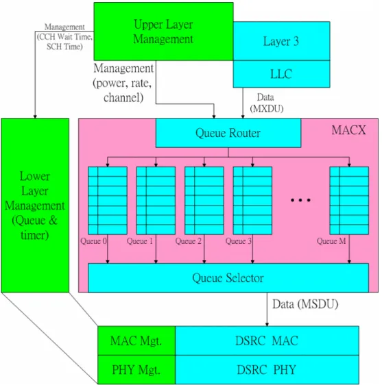
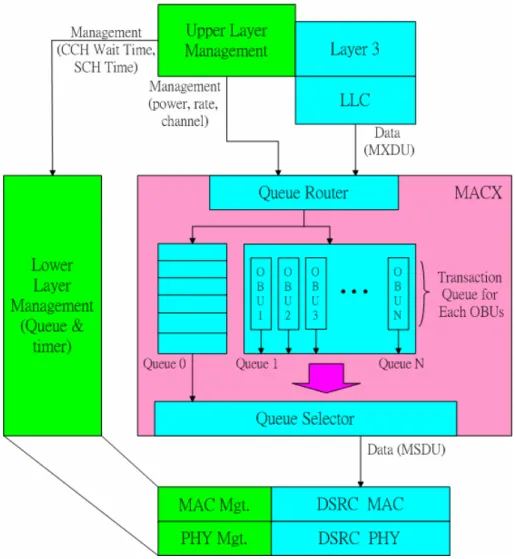
(12) supports the queuing of packets until an OBU returns to the SCH to complete the transactions in progress, as well as enforcing the requirement to return to the CCH [5].. Figure 1-1. Structure of the MAC extension and corresponding layer management for DSRC system. The structure of the MAC extension and corresponding layer management function for transmission operations is illustrated in Figure 1-1. For transmission of DSRC packets, each MAC extension data unit (MXDU) received by the MACX from the LLC layer is routed to a queue assigned to the channel where the packets is to be transmitted by queue router. In Figure 1-1, there are M queues corresponding to M SCHs and Queue 0 is corresponding to CCH. Beside channel assignment, the transmit power and data rate may also be controlled by 4.

(13) upper layer management. Using the interface to lower layer management, upper layer management can manipulate SCH Time and CCH Wait Time in the lower layer management [5]. RSU(s) and OBU(s) all implement these two timers in order to synchronize the RSU and OBUs to jump between CCH and SCH. According to the statement before, when the transaction in progress on the SCH is not completed before the SCH Time timer expires, the MACX will force to suspend the ongoing transmission returning to the CCH and wait for CCH Wait Time to listen for higher priority RST. The remaining packets are queued in the queue of the MACX. After CCH Wait Time timer expiring, the MACX will force the PHY back to SCH and queue selector selects the oldest MXDU from the non-empty queue(s). The queue selector’s operation behavior is with the first come first serve (FCFS). There are two kinds of communications in DSRC system. One is vehicle-to-vehicle (v2v) and another is vehicle-to-roadside (v2r). The IEEE 802.11 MAC protocol primarily supports communication on v2v and v2r SCHs, corresponding to two basic scenarios: an ad hoc mode characterized by distributed mobile multi-hop networking that allows vehicles in a fleet to communicate peer-to-peer directly; and an infrastructure mode characterized by a centralized mobile one-hop network for communication between vehicle to fixed roadside hubs. Therefore in v2r communications, RSU can work by using DCF mode or point coordination function (PCF) mode for high mobility environment [6]. In v2r communications, when RSU communicates with OBUs using CCH, they usually use DCF mode because there may be multiple OBUs and the overlapping RSU communication zones. When RSU communicates with OBUs using SCH, they can use any kinds of methods that both of them can support like PCF mode or others. In ITS service, RSUs are typically ITS application service providers, and OBUs are typically ITS application service users that get a lot of information from RSUs. At DSRC, the physical layer follows the IEEE 802.11a, the cell coverage is small, and the transmission data 5.

(14) rate is high. Besides, the speed of vehicles is fast. The occurrence of handoff is frequent and the dwell time in each cell is short. Therefore the service may hard to achieve continuity under this environment because of handoff failure. The handoff is a very important problem at DSRC. In this thesis, we design a downlink scheduling algorithm to address the handoff problem about the service that is provided via downlink direction at DSRC network. The algorithm we proposed can minimize the system handoff rate under satisfying the maximum tolerable delay requirement for the different kinds of application service.. 6.

(15) Chapter 2 Max Freedom Last Downlink Scheduling Algorithm Equation Section 2. 2.1. Introduction At DSRC network, the dwell time of a vehicle in a cell is short because of the small RSU communication zone and the high speed of the vehicle. Therefore the occurrence of handoff is frequent. In addition, the handoff latency is long; it will cause the system overhead heavy. The first reason for long handoff latency is that OBU need listen to the RST in CCH for detecting which RSU coverage area it locates and it can establish connection to which RSU to continue the incomplete service. Only until OBU listens to the RST and establishes the connection to the RSU, it can continuously be served by the target RSU. The second reason is the back-end signaling. When an OBU moves from one RSU coverage area to another, there are necessary to have some back-end signaling among the current RSU (sRUS), the target RSU (tRSU) and the authentication authorization accounting (AAA) server. The handoff problem is very important for DSRC with high mobility environment. As we mention before, DSRC adopts a WLAN based protocol. In WLAN, the handoff is commonly classified into two kinds. One is the inter-sub-net handoff and the other is the intra-sub-net handoff. The intra-sub-net handoff means that stations move from a basic service set (BSS) to another BSS but they are still in the same extended service set (ESS). The inter-sub-net handoff means that stations move across different ESS. For the inter-sub-net handoff, the DSRC system must have some requirements and structure to 7.

(16) support mobile IP service [7]. For the intra-sub-net handoff, the IEEE 802.11 WLAN system supports mobility across BSS boundaries. Mobile stations may move from one BSS to another and can maintain their higher-level network connections. This mobility is enabled through the use of IEEE 802.11 management frames and an inter access point protocol (IAPP) that is used to communicate on the distribution system (DS). In order to maintain the higher-level network connections for the mobile stations that move from one AP to another, APs must have interoperability within the DS. They are defined in IEEE 802.11F [8]. There are two directions to be considered to deal with the handoff problem. One is to reduce the handoff latency and the other one is to reduce the handoff rate. The meaning of reducing the handoff latency is to reduce the necessary time from the time that an OBU disconnects to one RSU to the time that this OBU establishes the connection to another RSU. There are many researches that take efforts to reduce the handoff latency. In [9], it proposed the prediction-based fast handoff scheme that supports broadband wireless access in fast moving vehicles. The proposed scheme supports seamless and fast handoff across continuous cells, and reduces packet loss across discontinuous cells. It used a concept that the moving pattern has a tendency to be predictable. Therefore the proposed scheme predicts handoff and next candidate access router in order to achieve seamless handoff. In [10], it introduced a fast handoff mechanism, NeighborCasting, for use in wireless IP networks that utilize neighboring foreign agent information. Initiating data forwarding to the possible new foreign agent candidates at the time that the mobile node initiates the link-layer handoff procedure minimizes handoff latency. In [11], it proposed a single protocol for both link layer (within IP subnet) and IP layer (across IP subnet) handoffs within a local domain. Combining routing table in IP layer and bridging table in link layer to form a single forwarding table, packets destined to a mobile terminal can be forwarded by simple table look-ups. Therefore the overhead and latency caused by interfacing the mobility management in link layer and IP 8.

(17) layer are eliminated. Then the proposed protocol can support fast and efficient link layer and intra-domain handoffs in the local domain. On the other hand, the meaning of reducing the handoff rate is to reduce the handoff occurrence probability among the duration that RSU provides the services to a lot of OBUs. In the DSRC lower layer management and MACX specification [5], a simple implementation method of the queue selector in the transmission mode is mentioned. All queues with the same priority are served on a FCFS basis. The oldest MACX data unit (MXDU) in the MAC extension queue(s) is delivered to the DSRC MAC in order of age. The queue selector is a function that chooses which queue and which MXDU to be delivered to MAC layer. It means that one transaction data can be served if it comes before the others regardless of the position and the velocity of the destination OBU or the volume of the whole transaction data. This method is not a good method because it may happen that OBUs leave for the sRSU cell coverage but the transaction data is not served completely yet and need to perform the handoff procedure. In [12] [13] [14], they considered the speed, location, and direction of the mobile stations to address some handoff problems. In [12], it presented a new policy of accepting the handoff calls that is optimal with respect to handoff failure probability and has the best channel utilization. In this scheme, the allocating channels prioritization of the handoff calls in queue was determined by their dwelling time in the handoff area. In [13], it proposed a handoff priority scheme called “Deadline Scheduling Queue” to process handoff requests. All mobile users have their deadline time (handoff threshold) according to their system parameter (speed direction of mobile travel, cell size and type of on-going mobile traffic). In [14], it proposed a handoff method that is fit for the pico-cellular networks called sub-group multicast-based handoff (SGMH). SGMH considers the MH’s (mobile host) speed and the distance from MH’s current location to the candidate handoff cells to reduce the buffer overhead and achieve seamless connection service. 9.

(18) In the real world, each OBU may have different velocity. And when an OBU has a request to RSU for downlink transmission data, it may be at different position at a cell and move different directions. Therefore the remaining dwell time of each OBU when it has a request to RSU for downlink transmission data may also be different. Someone may be long and someone may be short. If we can consider the position, moving direction and velocity of OBUs, we can schedule the transmission order of the OBU transactions suitably to reduce the handoff occurrence probability of OBUs. Besides, the volume of the transaction data must also be considered. If the data transmission rate is the same, the volume of the transaction data which is larger takes longer transmission time. Therefore if we consider these factors suitable to do scheduling for the service order of OBUs, we will reduce the handoff rate and then to reduce the system overhead. Usually the driver wants to get some information about driving or travels or others. RSUs are typically service provider and OBUs are typically service user. There we consider that RSU provides a service that downlink transmits data to OBUs that request from some information server in the Internet. Many OBUs may want to have request when the RSU provides this service. Therefore many OBUs may send response OSTs as the requests by using contention mechanism in WLAN when RSU sends RST of this service at CCH. After the RSU sends the ACKs to these response OSTs, they will jump to certain SCH to do downlink transmission service. As we mentioned before, FCFS is not a good method here. Therefore we think that RSU should consider both the remaining dwell time of each OBU and the remaining transmission time of each OBU transaction to schedule the transmission order of OBUs in order to reduce the handoff probability of OBUs. We consider that the RSU uses PCF mode (polling mode) in WLAN to perform the downlink transmission service for the OBUs in SCH. Then the service list generated by the scheduling algorithm we proposed would become the polling list in the PCF mode. 10.

(19) Data accessed in the ITS network are categorized into two types. One kind of data does not depend on the location of mobile hosts such as music, global news, and software programs etc. The other kind of data depends on the location of mobile hosts such as traffic information, detail driving map, and other travel information [15]. No matter what kind of data, data delay is important. If there is a too long time delay when the driver requests these data from the information center or the data server, the driver may request this information again or when the driver gets this information but this information becomes useless. Therefore, there should be a maximum tolerable timing delay for the service. And we should take the queueing delay for each OBU request data into account when we do the scheduling. In the thesis, our goal is to design a downlink-scheduling algorithm to minimize the system handoff rate under the maximum tolerable delay requirement. In this chapter, we propose a downlink-scheduling algorithm called max freedom last (MFL) scheduling algorithm to minimize the system handoff rate under the maximum tolerable delay requirement for the OBU transactions in DSRC system. The basic principle of MFL scheduling algorithm is to consider the complete served possible OBU first and then complete served impossible OBU. MFL serves the complete served possible OBUs with larger freedom later. And the algorithm increases the priority for OBUs according to the queueing delay and the maximum tolerable delay. The word “Freedom” means the degree of freedom for the possible complete service time of OBUs. When the RSU sends the RST to announce the downlink transmission service, OBUs can send OSTs to request information data in CCH and then jump to the SCH to start to receive the request data from RSU. Therefore each OBU has the necessary transaction time for receiving its request information data from RSU and the remaining dwell time before it moves out the sRSU coverage area. As long as OBUs can receive their request data completely from the RSU before they move out the sRSU coverage area, these OBUs are called completely served OBUs. We say that an 11.

(20) OBU has larger freedom if it has the less transaction time and the longer remaining dwell time. If an OBU has larger freedom, it can tolerate more OBUs served by RSU before it. Therefore we can achieve the goal for minimum handoff rate according to the degree of freedom. The proposed MFL scheduling algorithm will generate the service list and a data volume assignment table depending on the current conditions for OBUs including the remaining dwell time, the required transaction time and the queueing delay. In this thesis, the environment that we consider is that the vehicles are in the highway that is fully covered by the DSRC networks and the vehicles move for a bi-direction straight line. The RSU transmits the requested data to the OBUs via the downlink direction whenever OBUs request data from information servers or data servers. We consider an error free environment. And we assume that the remaining dwell time for each OBU can be obtained according to the moving direction, position and the velocity of OBUs. Also, the data transmission rate of the RSU is a fixed value and the service provided by RSU uses only one fixed SCH. In this thesis, we compare the MFL algorithm with the first-come-first-serve (FCFS) and the earliest deadline first (EDF) schemes in the aspects of system handoff rate, system utilization, and service failure rate. FCFS is a simplest operation method about the queue selector in the MACX sub-layer mentioned in the specification [5]. The RSU will serve the OBU whose request data first come to the queue for SCH in the MACX sub-layer of the RSU. EDF is another conventional method. There we define the deadline of EDF as the remaining SCH dwell time of each OBU. The RSU will serve the OBU, which has the shortest remaining SCH dwell time. When an OBU stays in the cell coverage of a RSU and waits for the RSU downlink transmission data to it, there are three kinds of results for the OBU: completely served, partially served, and completely un-served. The meaning of completely served is that the RSU downlink transmits the whole data that the OBU request before the 12.

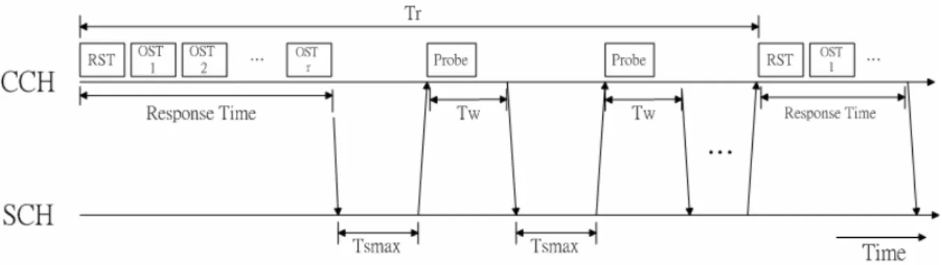
(21) OBU moves out this cell. The meaning of partially served is that the RSU transmits the partial data but still has some data in the queue when the OBU moves out this cell. The meaning of the completely un-served is that the RSU does not transmit any request data of the OBU before the OBU moves out this cell. When an OBU has request data not being completely served it will do the handoff and the remaining data in the queue will be forwarding to the next RSU. The rest of this chapter is organized as follows. At first, the system model that includes the system operation and the traffic model is described in section 2.2. The proposed scheduling algorithm is introduced in section 2.3. Finally, the simulation result and concluding remarks are presented in section 2.4 and 2.5, respectively.. 2.2. System Model 2.2.1. System Operation The system environment we considered is the DSRC network covering highway, and the vehicles move in a bi-direction straight line with different velocity. The RSUs’ coverage areas are lightly overlapped, and the RSUs provide the service of transmitting data to OBUs.. Figure 2-1. Signaling Operation. RSU will send the RST in CCH to announce this service and OBUs may request for service 13.

(22) by sending OSTs to response the RST. Figure 2-1 shows the diagram of the signaling operation. In this figure, Tr is the period of the RST transmission and TSMAX is the maximum SCH time. The maximum SCH time means the uninterrupted duration that both RSU and OBUs can stay at the SCH. Tw is the CCH wait time, which is the duration that the RSU and the OBUs get to monitor the CCH. At the beginning, the RSU sends the RST in CCH to announce the service that it provides. Then OBUs, which have interest to the service, send the OSTs responses to the RSU to request data transmission and contend with other OBUs. If the RSU successfully receives an OST and can accept the request, RSU will response an ACK to the OBU. The duration that OBUs can send OSTs is called the response time. We set the value of the response time equal to Tw . In each time that RSU sends the RST, it permits that a maximum number of OBUs that can send OSTs at the response time period. This value is equal to r . If there are r OSTs sent by OBUs, the RSU will response the next OST by broadcasting an NACK and the OBUs that request success would jump to SCH to begin the service. There is a high priority service provided by RSUs for OBUs to do registration to the RSUs. In WLAN, when a station moves from one AP to another and listens to the beacon sent by the new AP, it will send the re-association request to the new AP in order to register and ask to establish the connection. Then the new AP will send the re-association response to the station and completely establish the connection. But in DSRC, there are no beacons sent by RSUs. If RSUs want to provide some service, they will send the RST to announce. Therefore the function of the RST in DSRC is like the function of beacon in WLAN. When an OBU powers on or moves from one RSU to another one, it listens to this kind RST for registration service and responses OSTs to do association request or re-association request. If handoff OBUs arrival in this cell, they must register to the RSU and accomplish the handoff procedure first. After that, when the handoff OBU listens to the RST for service, it 14.

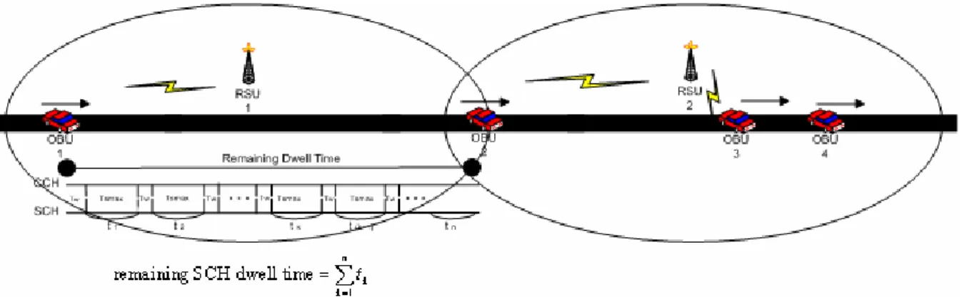
(23) can directly jump to SCH to begin the service together without requesting again. Therefore the total number of OBUs that RSU admits to serve is equal to the number of handoff OBUs plus the number of new OBUs and the OBUs that are still not served completely. When all the accepted OBUs jump to SCH, RSU will do scheduling first and then serve these OBUs based on the scheduling result. At the same time, the SCH Time timer starts to decrease from Ts max . When SCH Time timer expires, the RSU and these OBUs suspend their transmission and return to CCH to monitor. Hereafter the in-process OBU will send a probe and the other timer CCH Wait Time will start to decrease. If there is a high priority service provided by the RSU, the RST responds to this service after the probe. If no other urgent or important service happens, the RSU and OBUs will return to the SCH and resume the suspension service. In DSRC, the RSU and OBUs can not always stay in SCH to do communication because they need to monitor the CCH for the high priority service. But the RSU can only transmit data for OBUs in SCH. Therefore we need to transfer the remaining dwell time to the remaining SCH dwell time as the input for MFL algorithm. Now we describe the relationship between them.. Figure 2-2. The relationship between the remaining dwell time and the remaining SCH dwell time Figure 2-2 illustrates the relationship between the remaining dwell time and the 15.

(24) remaining SCH dwell time. The remaining SCH dwell time is equal to the remaining dwell time of OBUs in this cell deducting the total CCH Wait Time Tw and the OBU response time within the remaining dwell time of OBUs. In our system, the value of the response time is equal to Tw . Therefore we can obtain a transformation function to transfer from the remaining dwell time to the remaining SCH dwell time. The transformation relationship between the remaining dwell time and the remaining SCH dwell time is as follows:. ⎧ ⎛ ⎢ DTi ⎥ ⎞ ⎢ DTi ⎥ ⎪ DTi − ⎜ ⎢ ⎥ * ( p + 1) + 1⎟ * Tw , if DTi − ⎢ ⎥ * Tr > Tw T T r r ⎣ ⎦ ⎣ ⎦ ⎪ ⎝ ⎠ Di = ⎨ , ⎛ ⎞ ⎢ ⎥ ⎢ ⎥ DT DT ⎪ i i ⎪⎜ ⎢ T ⎥ * ( p + 1) ⎟ * Ts max , if DTi − ⎢ T ⎥ * Tr ≤ Tw ⎣ r ⎦ ⎠ ⎩⎝ ⎣ r ⎦. (2.1). Tr = ( p + 1) * (Tw + Ts max ) ,. (2.2). where p is the number of the probe between two RSTs, Di is the remaining SCH dwell time for OBU i , DTi is the remaining dwell time for OBU i , Tr is the repeat period of the RST transmission, and Ts max is the maximum uninterrupted duration of an SCH transaction, and Tw is the period of time that an OBU listens on the CCH before returning to a SCH. So the remaining dwell time is equal to the remaining SCH dwell time considers the absolute time axis. We describe the handoff procedure for the handoff OBUs. When a handoff OBU moves to a RSU coverage area, it will listen to the RST for registration service. After it listens to the registration RST, it sends the OST to do re-association. When the RSU receives the OST, it accomplishes the registration and starts the handoff procedure. RSU will send an IAPP-MOVE-Notify packet to the previous RSU that this OBU associates to inform the previous RSU that an OBU moves into here and performs the re-association. Then the previous RSU will forward the remaining data of the handoff OBU stored in the queue to the new RSU. Then the previous RSU sends the IAPP-MOVE-Response packet to the new RSU and release the resource that allocates to this OBU. In IEEE 802.11F [8], it defines a 16.

(25) proactive caching method. It can transfer the user context in advance. Therefore when a handoff OBU moves into the new RSU coverage area, it can establish the connection quickly.. Figure 2-3. System Operation. 17.

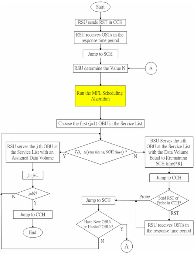
(26) Figure 2-3 is the flow chart of the system operation. When RSU sends RST in the CCH, RSU waits to receive OSTs in the response time. The OBUs that have interest to the service will respond with OSTs by contending with other OBUs. Then the RSU and these OBUs which have request for service jump to SCH to begin the service. The RSU determine the value N that is the total number of OBUs needed to be scheduled. This N includes the new OBUs, the handoff OBUs in this round and the OBUs that came before. Afterwards, RSU runs the MFL scheduling algorithm to determine the service list and data volume assignment table. TDs j is the transmission time of the assigned data volume of the j-th OBU transaction at the service list. If TDs j is smaller than or equal to the remaining SCH Time, the assigned data of the j-th OBU transaction can be served completely without interruption by monitoring the CCH. Otherwise, RSU only transmits part of the assigned data for the j-th OBU transaction and jumps to CCH to monitor. TDs j is equal to the data volume that records in the data volume assignment table for the j-th OBU transaction divided by the data transmission rate R . When the RSU and OBUs jump to CCH, the in-process OBU will send probe or the RSU will send the RST. If there are new OBUs or handoff OBUs arrival after the RSU sends the RST, the MFL scheduling algorithm will run again because the system condition is changed. Otherwise, the RSU and OBUs jump back to the SCH to continue the service. If all OBUs at the service list are served completely, the service will be end and RSU will jump back to CCH to wait for next time to transmit the RST. The layer architecture of protocol for the RSU is illustrated in Figure 2-4. There are one CCH queue (queue 0) and a group of transaction queues for each OBUs queue i for OBU i , 1 ≤ i ≤ N . The remaining portion is the same as the structure of the MAC extension and. corresponding layer management structure in Figure 1-1. In order to reduce the handoff rate of OBU at the DSRC system, RSU should consider 18.

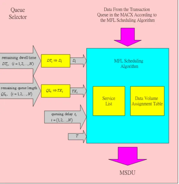
(27) OBUs’ position, moving direction and velocity, and the data volume of the OBU transactions in the design of scheduling. The proposed scheduling algorithm will generate a service list and a data volume assignment table. The service list determines the transmission order of OBUs and the data volume assignment table records the served data volume allowed for OBUs in the service list. The queue selector chooses which OBU’s data to be transmitted according to proposed scheduling algorithm.. Figure 2-4. The layer architecture in RSU. Figure 2-5 shows the detailed structure of the queue selector. The queue selector mainly contains the proposed scheduling algorithm. The MFL scheduling algorithm will generate a service list and a data volume assignment table according to the remaining SCH dwell time, 19.

(28) the remaining transmission time, the queueing delay for each OBU, and the maximum tolerable delay for the service.. Figure 2-5. Detailed structure of the Queue Selector. In the figure, DTi is the remaining dwell time for OBU i , QLi is the remaining queue length for OBU i , and ti is the queueing delay for OBU i , 1 ≤ i ≤ N . This information is collected from OBUs. Before this information inputs into the MFL algorithm, RSU transfers the remaining dwell time DTi to the remaining SCH dwell time Di and converts the remaining queue length QLi to remaining transmission time TX i . The relationship between QLi and TX i is given by: 20.

(29) TX i =. QLi , R. (2.3). where R is the transmission data rate of the RSU. The relationship between DTi and Di is described in equation (2.1). Also, there is still one input system parameter T , where T is the maximum tolerable delay for the service provided by the RSU. Then the queue selector selects MSDUs to transmit according to the algorithm result. There are two kinds of OBUs that arrival to the RSU in the system, new OBUs and handoff OBUs. The new OBUs are the OBUs that just send OSTs to response the RST in the response time in CCH and are accepted by the RSU. The handoff OBUs are the OBUs that are partially served or completely un-served by the previous RSU and move into a new RSU (tRSU) coverage area. When the handoff OBUs move into tRSU, they will listen to the RST for the registration first. Then the handoff procedure starts. The handoff procedure follows the IAPP protocol defined in IEEE 802.11F. After registration, the handoff OBUs can be scheduled by RSU without doing contention with other new OBUs.. 2.2.2. Traffic Model Here we model the sending process that OBUs send OSTs to response the RST in CCH as a Poisson process. Denote the number of the new OBUs requests by N n , which is Poisson random variable with mean value µ n . And each request for OBUs will bring a burst data. Denote the number of the MSDU data for each new OBU request by N p , which is a truncated Pareto distribution defined as:. fNp. ⎧ α kα , m > np > k , ⎪ , ( n p ) = ⎨ n pα +1 ⎪β , n p = m, ⎩. (2.4). where m is the maximal allowed number, k is the minimal allowed number, α is the 21.

(30) parameter for Pareto distribution, and β is the probability that n p > m . It can be calculated as: α. ⎛k⎞. β = ∫ f N ( n p ) dn p = ⎜ ⎟ ,α > 1, m ⎝m⎠ ∞. (2.5). p. Then we can obtain the mean of the MSDU number as: α. ∞. µN = ∫ np f N p. −∞. p. ⎛k⎞ αk − m⎜ ⎟ ( n p ) dn p = α −⎝1m ⎠ ,. (2.6). We describe the definitions of three performance index observed in the simulation result. The definition of the system handoff rate is given by: Rsh =. N ps + N cu N ps + N cu + N cs. ,. (2.7). where Rsh is system handoff rate, N ps is the number of the partially served OBUs, N cu is the number of the completely un-served OBUs, and N cs is the number of the completely served OBUs in the overall system. The definition of the system utilization is the average ratio of the RSU data transmission time per time unit. As we mention before, our goal is to design a downlink-scheduling algorithm to minimize the system handoff rate under the maximum tolerable delay requirement. If an OBU is not completely served by the system before the maximum tolerable delay, the service that the OBU requests will become failure. The definition of the service failure rate is given by: Rsf =. N sf N srd. ,. (2.8). where Rsf is service failure rate, N sf is the number of the service failure OBUs, and N srd is the number of the all OBUs accepted by RSU. The successful request data OBUs means the OBUs that request data to the RSU and the RSU sends response to it for acceptation.. 22.

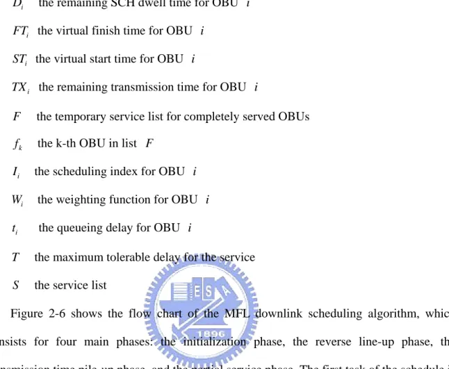
(31) 2.3. MFL Downlink Scheduling Algorithm The downlink scheduling algorithm generates a service list and a data volume assignment table. We consider the remaining SCH dwell time, the remaining transmission time, and the queueing delay of the request data for each OBU and the maximum tolerable delay for the provided service to design the algorithm. The goal of the downlink scheduling algorithm is to minimize the system handoff rate under the maximum tolerable delay requirement for the service and make full utilization of the SCH. To minimize the system handoff rate is equivalent to maximize the number of completely- served OBUs in the system. Therefore, the algorithm first serves the OBUs which can be possibly served completely and then serves other OBUs if there is any remaining resource. Since each OBU has its remaining SCH dwell time and data transmission time, an OBU is completely served if the total request data of an OBU is transmitted by RSU before it moves out this cell. Besides, when the queueing delay becomes large, we should increase the priority for OBUs to let the queueing delay not exceed the maximum tolerable delay. The proposed scheduling algorithm will consider the remaining SCH dwell time, the remaining transmission time, and the queueing delay of the request data for each OBU and the maximum tolerable delay for the provided service to achieve better performance. Before we design the scheduling algorithm, some notations that will be used in the MFL scheduling algorithm are defined: A. the set of all OBUs that we consider in the establishment of the MFL scheduling algorithm. A+. the set of the OBUs that have a chance of being completely served. A−. the set of the OBUs that have no chance of being completely served. k. the index of the list F. i. the index of the OBU 23.

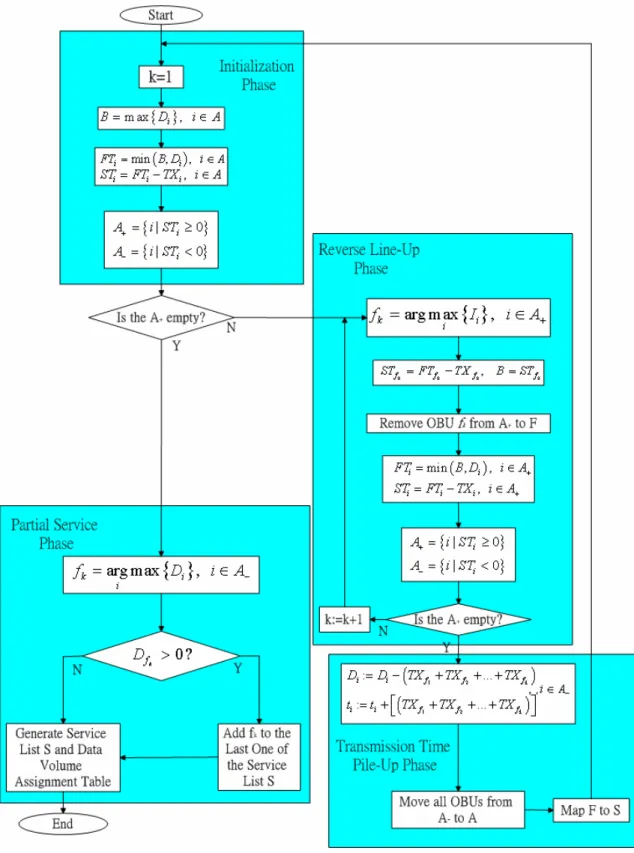
(32) B. the limit bound of the remaining SCH dwell time for all OBUs in set A+. Di. the remaining SCH dwell time for OBU i. FTi the virtual finish time for OBU i STi the virtual start time for OBU i TX i the remaining transmission time for OBU i. F. the temporary service list for completely served OBUs. fk. the k-th OBU in list F. Ii. the scheduling index for OBU i. Wi. the weighting function for OBU i. ti. the queueing delay for OBU i. T. the maximum tolerable delay for the service. S. the service list. Figure 2-6 shows the flow chart of the MFL downlink scheduling algorithm, which consists for four main phases: the initialization phase, the reverse line-up phase, the transmission time pile-up phase, and the partial service phase. The first task of the schedule is to determine a set A+ in which the OBUs may be completely served. The initialization phase sets the initial values of the virtual finish time FTi and virtual start time STi for each OBU i , and partitions all OBUs into sets A+ and A− . In the reverse line-up phase, the algorithm then constructs the temporary service list F according to the value of the scheduling index I i of all OBUs, where i ∈ A+ . For each iteration in the reverse line-up phase, the algorithm calculates the virtual start times for all OBUs in A+ to check if any OBU becomes not to be completely served. After the A+ is empty, the procedure enters the transmission time pile-up phase. All the gaps between any two consecutive transmissions are compacted and all transmission periods are piled up and concatenated together. After the transmission time pile-up phase, the procedure enters back to the initialization phase to check 24.

(33) whether there is remaining resource for OBUs to be completely served or not, the above phases will be performed iteratively till no further OBUs classified into the set A+ in the initialization phase. If there is no OBU in the set A+ , the procedure will enter the partial service phase. If there exists any OBUs whose remaining SCH dwell time is larger than zero, one OBU in A- will be scheduled. Finally, the complete service list S is determined and the scheduling is finished. In the initialization phase, the algorithm partitions all OBUs into sets A+ and A− , where A+ consists of all OBU i whose virtual start time STi is not negative and A− consists of all OBU i whose virtual start time STi is negative. The virtual start time STi for OBU i is given by: STi = FTi − TX i ,. (2.9). where FTi is the virtual finish time for OBU i and TX i is the remaining transmission time for OBU i . The value of FTi is equal to the remaining SCH dwell time Di in the initialization phase. Therefore an OBU may be completely served if its value of the virtual start time is larger than or equal to zero. In the reverse line-up phase, the algorithm generates the temporary service list F . The procedure to form the temporary service list F is as follows: Define. {k = 1. FTi = Di , ∀i ∈ A+ }. step 1 : f k = arg max { I i } i. step 2 : ST fk = FT fk − TX fk , B = ST fk step 3 : A+ := A+ − { f k } step 4 : FTi = min { Di , B} STi = FTi − TX i , ∀i ∈ A+ step 5 : A+ = {i | STi ≥ 0} , A− = {i | STi < 0} step 6 : If. A+ ≠ ∅ k = k + 1 goto step 2. step 7 : End The temporary service list F is as a linked list data structure which is constructed by an iterative sorting procedure. In each iteration, the OBU with the largest scheduling index is 25.

(34) found, then put into F and removed from the A+ . Afterwards, parameters of remaining OBUs in A+ are re-calculated, and the sorting procedure restarts. This iterative procedure of this phase ends till the A+ is empty. In the initialization phase, k is set to be one and the virtual finish time for OBU i , FTi , is equal to its own remaining SCH dwell time, i ∈ A+ . The step 1 is to choose an OBU which has the maximum scheduling index I i among A+ and put it in the list F , in the k th iteration. The scheduling index I i for OBU i is given by:. I i = FTi − Wi * TX i ,. (2.10). where Wi is the weighting function for OBU i . The weighting function Wi is defined as: ⎧ ti ' ⎪⎪1 − T , if T − ( FTi + ti ) ≥ 0 Wi = ⎨ , t ' i ⎪1 + , if T − ( FT + t ) < 0 i i ⎪⎩ T. (2.11). where FTi ' is defined in (2.1) which is the virtual finish time on the absolute time axis, ti is the queueing delay for OBU i , and T is the maximum tolerable delay for the service. The algorithm calculates the scheduling index for all OBUs. If the service time (waiting time + transmission time) of OBU i exceeds the maximum tolerable delay, the value of its weighting function Wi will be larger than one. Otherwise, the value of its weighting function Wi will be smaller than or equal to one. The effect will decrease or increase the scheduling index. Consequently, an OBU with larger queueing delay but within the maximum tolerable delay has larger probability to be chosen by the algorithm. The step 2 calculates the virtual start time for OBU f k . This value will be the limit bound B of the remaining SCH dwell time for all OBUs in set A+ at the next sorting iteration. The step 3 removes OBU f k from the set A+ . In step 4, after OBU f k is selected to be in the list F , the algorithm computes the virtual finish time for all OBUs in set A+ given by: 26.

(35) FTi = min ( B, Di ) ,. Figure 2-6. The flow chart of the MFL downlink scheduling algorithm. 27. (2.12).

(36) In order to serve most OBUs completely, the algorithm sets the virtual finish time of each OBUs close to its remaining SCH dwell time as much as possible. However, if the remaining SCH dwell time of an OBU is larger than the bound B , the virtual finish time only will be set by B . Also, the virtual start time for all OBUs in set A+ is calculated to check if any OBU can not be completely served. In step 5, all OBUs are re-partitioned. The OBUs with virtual start time not less than zero belong to the set A+ , otherwise A− . The step 6 checks whether all possible completely served OBUs are totally selected in this round of iterations. If it is right, the temporary service list F is formed and the MFL algorithm procedure will enter the transmission time pile-up phase. In the transmission time pile-up phase, the remaining SCH dwell time for each OBU in set A− is set equal to the original value minus the sum of the remaining transmission time for all OBUs in the list F , and the queueing delay for each OBU in set A− is set to the original value plus the value that the sum of the remaining transmission time on the absolute time axis for all OBUs in the list F . All OBUs in the set A− move to the set A . And then the OBUs in the list F move to the service list S . The rule for moving OBUs from the list F to the service list S is like the behavior of the stack using the rule as first in last out. It is because that the algorithm schedules the completely-served OBUs by sorting the service order of OBUs in a reverse order so that the reverse order of list F is equal to the order of the service list S . After this phase, the algorithm gets back to the initialization phase to check if any OBU can be served completely. If the algorithm completes the sorting procedure for completely served OBUs, the algorithm enters into the partial service phase. The algorithm selects the OBU in set A− with the maximum remaining SCH dwell time. If the value of this OBU is larger than zero, it means that this OBU can be partially served. The algorithm adds this OBU in the last of the 28.

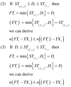
(37) service list S and assigns the data volume for this OBU to be its remaining SCH dwell time multiplies the transmission rate. Finally, the service list is generated. The process to construct the MFL scheduling algorithm is to iteratively sort OBUs in a reverse order according to the scheduling index. In the following, we will prove that the reverse mechanism in the reverse line-up phase can achieve the minimum system handoff rate. The proof is performed at the condition that neglects the queueing delay, which means that the weighting function is equal to one. In addition, the meaning of the minimum system handoff rate is equal to serving the maximum number of OBUs. The proof uses the mathematical induction method. Main Result:. The process in the reverse line-up phase can serve the maximum number of completely served OBUs. <Pf> In the following proof, denote N to be the number of OBUs in the list A+ , the notation “. ( ). '. ” to be a process using the other policy, and notation “ n (U i ) ” to be the. number of OBUs that satisfy the condition U i ≥ 0 .. I: Basis of induction : k = 1 means the 1st iteration of the reverse line-up phase. The correctness that RSU can serve the maximum number of completely served OBUs for k = 1 is proved in the following way : When k = 1 , we have FTi = Di f1 = arg max { FTi − TX i } , i. (. ( f1 ). '. ≠ f1 ∀i ∈ A+ , STi ≥ 0. ). ST f1 = ( FT f1 − TX f1 ) ≥ FT( f )' − TX ( f )' = ST( f )' . 1. 1. 1. Then we divide the relation of ST f1 , ST( f )' and Di into three cases. 1. (1) If ST( f )' ≤ ST f1 ≤ Di then 1. FTi = min {ST f1 , Di } = ST f1 29.

(38) ( FTi ). {. }. = min ST( f )' , Di = ST( f )'. '. 1. we can derive. (. 1. n ( FTi − TX i ) ≥ n ( FTi ) − TX i '. ). (2) If ST( f )' ≤ Di ≤ ST f1 then 1. FTi = min {ST f1 , Di } = Di. ( FTi ). '. {. }. = min ST( f )' , Di = ST( f )' 1. we can derive. (. 1. n ( FTi − TX i ) ≥ n ( FTi ) − TX i '. ). (3) If Di ≤ ST( f )' ≤ ST f1 then 1. FTi = min {ST f1 , Di } = Di. ( FTi ). '. {. }. = min ST( f )' , Di = Di 1. we can derive. (. n ( FTi − TX i ) ≥ n ( FTi ) − TX i '. ). Therefore the result for k = 1 is proved. II: Inductive hyposis : We assume that when k = x the result is correct for 1 < x < N − 1. III: Inductive step : If the result is correct when k = x then we have. {. FTi = min ST f x , Di. }. When k = x + 1 for 1 < x < N − 1 we can obtain f x +1 = arg max { FTi − TX i } , i. (. ( f x+1 ). (. ). ST f x +1 = FT f x +1 − TX f x +1 ≥ FT( f. x +1. )'. '. ≠ f x +1 ∀i ∈ A+ , STi ≥ 0. − TX ( f. Then we divide the relation of ST f x +1 , ST( f (1) If ST( f. x +1. )'. ≤ ST f x +1 ≤ Di then. {. }. FTi = min ST f x +1 , Di = ST f x +1. ( FTi ). '. {. = min ST( f. we can derive. (. x +1. )'. }. , Di = ST( f. n ( FTi − TX i ) ≥ n ( FTi ) − TX i '. x +1. ) 30. )'. x +1. x +1. )'. )'. ) = ST. ( f x +1 )'. .. and Di into three cases..

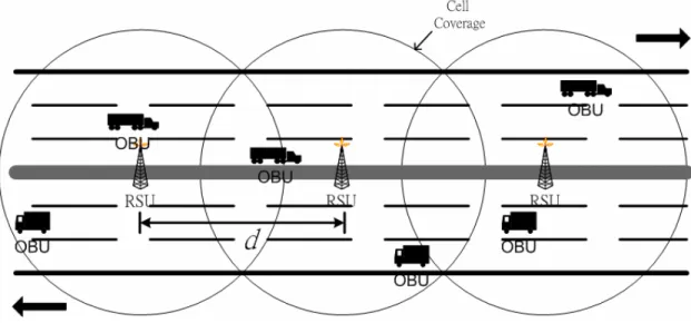
(39) (2). If ST( f. x +1. )'. ≤ Di ≤ ST f x +1 then. {. }. FTi = min ST f x +1 , Di = Di. ( FTi ). '. {. = min ST( f. we can derive. x +1. )'. }. , Di = ST( f. (. n ( FTi − TX i ) ≥ n ( FTi ) − TX i (3). If Di ≤ ST( f. {. x +1. )'. '. x +1. )'. ). ≤ ST f x +1 then. }. FTi = min ST f x +1 , Di = Di. ( FTi ). '. {. = min ST( f. we can derive. x +1. )'. }. , Di = Di. (. n ( FTi − TX i ) ≥ n ( FTi ) − TX i '. ). Therefore the result for k = x + 1 is proved.. Therefore this procedure in MFL algorithm can achieve the minimum system handoff . rate.. 2.4. Simulation Result 2.4.1. Simulation Environment Figure 2-7 shows the simulation environment, where a six-lane highway is considered. All the vehicles in the highway move in either one direction and they do not turn around. RSUs are uniformly put at the center of the highway, and the distance between two RSUs is equal to d . The long-term fading effect is considered in the simulation. The process that the new OBUs send OSTs to respond the RST is modeled as a Poisson Process with mean value µ n . And the MSDU number of the burst data requested by each new OBU is a truncated Pareto distribution with a parameter α . The minimal MSDU number of the burst data is k , the maximal number is m , and the size of an MSDU is M 31.

(40) bytes.. Figure 2-7. Simulation Environment. OBUs send OSTs to request for data service. The positions that OBUs send OSTs are uniformly located within the coverage of the RSU. The velocity of each vehicle with OBU is with uniform distribution with minimal velocity Vmin and maximal velocity Vmax . The system parameters are described as follows:. System Parameters. Notation. Value. The distance between two RSUs. d. 400 m. The mean arrival rate of the request data OBUs. µn. 2/sec. The parameter of the Pareto distribution. α. 1.1. The minimal number of MSDU of the request data. k. variable. The maximal number of MSDU of the request data. m. 10000. The size of each MSDU. M. 1000 bytes. The minimal velocity of vehicles. Vmin. 60 km/hr. 32.

(41) The minimal velocity of vehicles. Vmax. 120 km/hr. The maximum SCH Time. Ts max. 100 ms. CCH Wait Time. Tw. 5 ms. Repeat period of the RST transmission. Tr. 1050 ms. The maximal number of accepted OBUs per RST. r. 4. The maximum tolerable delay. T. variable. Data transmission rate. R. 18 Mbps. The number of probes between two RSTs. p. 9. Table 2-1. System Parameters. 2.4.2. Simulation Result and Conclusion In the simulation, we compare the proposed MFL algorithm with FCFS and EDF. Figure 2-8 and Figure 2-9 show the service failure rate versus the mean data size if using these three algorithms, where the maximum tolerable delay T is equal to 60s in Figure 2-8 and the maximum tolerable delay T is equal to 180s in Figure 2-9. Mean data size denotes the average volume of the burst data that an OBU requests information service which is calculated according to equation (2.6). We can see that MFL has smaller service failure rate than FCFS and EDF. The service failure rate is zero for three methods when the mean data size is below about 900k bytes. It is because that the system utilization is still light, thus almost all OBUs can be completely served within the maximum tolerable delay bound. The service failure rate for three methods starts to increase from zero when the mean data size is larger than around 900k bytes. It can be seen that MFL has the lowest service failure rate while FCFS has the largest. There are two reasons for this result. The first one is that MFL is the best policy to achieve the minimum system handoff rate. OBUs will have lower probability to become service failure. 33.

(42) Figure 2-8. Service Failure Rate for T = 60 s. Figure 2-9. Service Failure Rate for T = 180 s. This result will be showed later. And the other one is that MFL will let OBUs, which have 34.

(43) longer queueing delay and are closer to the maximum tolerable delay, have higher probability to be served. The method is by virtually decreasing the remaining transmission time of OBU. On the other hand, EDF and FCFS do not have any reaction when OBUs have longer queueing delay which is close to the maximum tolerable delay. Our goal is to design a downlink scheduling algorithm for DSRC networks in order to minimize the system handoff rate under the maximum tolerable delay requirement. Therefore the service failure rate must be limited in a reasonable range. If the required service failure rate is set at 0.1, the curves of three methods that meet this requirement are meaningful.. Figure 2-10. System Utilization for T = 60 s. Figure 2-10 and Figure 2-11 show the system utilization versus the mean data size for the three algorithms with the maximum tolerable delay is equal to 60s and 180s, respectively. It can be seen that the three methods can achieve the same system utilization. RSU can transmit data for OBUs if the transaction queues are not empty. And three methods use the same acceptation rule for OBUs. Therefore three methods can achieve the same system 35.

(44) utilization.. Figure 2-11. System Utilization for T = 180 s. According to the figure of the system utilization, we divide each following figures into three regions to observe and discuss. The first region is the range of the mean data size from 400 kbytes to the size of 800 kbytes at which the system is at light load. The second region is the range of the mean data size from 800 kbytes to the size of 1000 kbytes at which the system is at medium load. The third region is the other region of the mean data size from 1000 kbytes to 1200 kbytes at which the system load is heavy. Figure 2-12 and Figure 2-13 show the system handoff rate versus the mean data size for the three algorithms with the maximum tolerable delay equal to 60s and 180s, respectively. It can be seen that in the first region of Figure 2-12, MFL has smaller in the system handoff rate than FCFS but is almost the same as compared to EDF. In the second and third regions, MFL has the system handoff rate better than EDF. And the difference between MFL and EDF turns to be larger if the mean data size becomes larger. 36.

(45) Figure 2-12. System Handoff Rate for T = 60 s. Figure 2-13. System Handoff Rate for T = 180 s. In Figure 2-13, the behavior of the first and the second regions is the same as Figure 2-12. In the third region, although MFL is still better than FCFS and EDF in the system 37.

(46) handoff rate, the difference between MFL and EDF becomes smaller. We compare with Figure 2-12 and Figure 2-13. It can be seen that when we increase the maximum tolerable delay from 60s to 180s, the system handoff rate of three methods for all mean data size points becomes larger. Then we explain why the increasing rate of EDF in the service failure rate is slower than FCFS in Figure 2-8 and Figure 2-9. First, both FCFS and EDF do not have a reaction to the queueing delay and think about the maximum tolerable delay. And in Figure 2-12 and Figure 2-13, we can see that EDF is better than FCFS in the system handoff rate. It means that EDF has better ability to determinate the service order for OBUs than FCFS. Therefore EDF has lower probability to let OBUs become failure than FCFS. So the increasing speed of EDF in the service failure rate is slower than FCFS. As we mentioned before, we divide the OBUs into two kinds, new OBU and handoff OBU. We can individually observe to the new OBU and handoff OBU in the handoff rate. And the result of the system handoff rate comes from combining the new OBU handoff rate and the handoff OBU handoff rate according to the number of new OBUs and handoff OBUs. Therefore in the following, we observe and discuss about the new OBU handoff rate and the handoff OBU handoff rate in order to explain the system handoff rate. Figure 2-14 and Figure 2-15 show the new OBU handoff rate versus the mean data size for the three algorithms with the maximum tolerable delay equal to 60s and 180s, respectively. In the first region of Figure 2-14 and Figure 2-15, it can be seen that the new OBU handoff rate of FCFS increases faster than EDF and MFL. It is because that FCFS does not consider either the remaining SCH dwell time or the remaining transmission time. Also, MFL and EDF have almost the same new OBU handoff rate. It is because that the mean data size is still small in the first region, and thus the remaining transmission time is much less than the remaining SCH dwell time. As we mentioned before, MFL schedule OBUs according to the scheduling index I i . If the mean data size is small, the scheduling index 38.

(47) will become almost equal to the remaining SCH dwell time. Therefore the result of MFL and EDF will become almost the same.. Figure 2-14. New OBU Handoff Rate for T = 60 s. Figure 2-15. New OBU Handoff Rate for T = 180 s 39.

(48) In the second and third regions, the increasing rate of the new OBU handoff rate in MFL is slower than EDF. It is because the effect of the remaining transmission time considered in MFL becomes obvious. And the increasing speed of FCFS is still faster than EDF. The reason is mentioned before. Then we compare Figure 2-14 and Figure 2-15. It can be found that the performance results for three methods are almost the same individually in the first region. It is because that in the first region the system is at light load and the service failure rate is zero for the three methods. When we increase the maximum tolerable delay from 60s to 180s, the number of handoff OBU only has small increment and the new OBU handoff rate will not be affected at all. But in the second and third regions, the system is at medium and heavy load and the service failure rate starts to increase from zero. There is more and more handoff OBUs in the system. If the maximum tolerable delay is increased, OBUs can tolerate longer waiting time before service failure. Therefore the number of handoff OBU will become larger and the new OBU handoff rate will become higher. Figure 2-16 and Figure 2-17 show the handoff OBU handoff rate versus the mean data size for the three algorithms with the maximum tolerable delay equal to 60s and 180s, respectively. In both figures, it can be seen that the handoff OBU handoff rate of FCFS is almost close to zero in the first region. It is because that the system is still at light load and the handoff OBUs have the highest priority in FCFS. As we mentioned before, when a handoff OBU moves to tRSU, it must register to the tRSU first. After it completes the handoff procedure, its remaining data will be forwarded from sRSU to tRSU. And then it can be scheduled when the RSU sends the next RST. Therefore the handoff OBU data will always come to the RSU before the new OBU data in a round.. 40.

(49) Figure 2-16. Handoff OBU Handoff Rate for T = 60 s. Figure 2-17. Handoff OBU Handoff Rate for T = 180 s. We compare Figure 2-16 and Figure 2-17. It can be found that when the maximum tolerable delay is increased from 60s to 180s, the handoff OBU handoff rate for three 41.

(50) methods will all become higher. The reason is that when we increase the maximum tolerable delay, there is more handoff OBUs staying in the system but the time of RSU for transmission data is the same. Besides, it can be seen that the increasing degree of handoff OBU handoff rate in MFL is larger than other two methods. The reason is that the priority for OBUs that have longer queueing delay is increased according to the ratio of the queueing delay over the maximum tolerable delay. Thus as the maximum tolerable delay is increased, the degree of priority increment for handoff OBUs will decrease. We observe the figures for the new OBU handoff rate and the handoff OBU handoff rate. It can be found that MFL is better than EDF and EDF is better than FCFS in new OBU handoff rate. But the order is reverse in handoff OBU handoff rate. It is because that the total time that RSU can transmit data for OBUs is fixed. Consequently, the new OBU and handoff OBU can not be kept in mind at the same time. Finally, we come back to see the performance of system handoff rate. For three regions in Figure 2-12, the performance behaviors for the three methods are dominated by the new OBU handoff rate. However, for the first region in Figure 2-13, the performance behaviors are dominated by the new OBU handoff rate. But for the second and the third regions in Figure 2-13, the performance behaviors are dominated by the handoff OBU handoff rate. It is because that when we increase the maximum tolerable delay from 60s to 180s, the number of the handoff OBU will increase significantly.. 2.5. Concluding Remarks In this chapter, a max freedom last (MFL) downlink scheduling algorithm is proposed for DSRC networks. The MFL scheduling algorithm can minimize the system handoff rate under a maximum tolerable delay for the service. We also give a proof that the process in the reverse line-up phase can minimize the system handoff rate. Simulation results show that the 42.

(51) MFL scheduling algorithm has better performance in the service failure rate and the system handoff rate than FCFS and EDF. This is because the MFL scheduling algorithm considers the remaining SCH dwell time, the remaining transmission time, and the queueing delay for all OBUs. Therefore the MFL scheduling algorithm can deal with the mobility issue at DSRC networks and reduce the system overhead.. 43.