線段移動及鏡相繞線技術應用於全域繞線器

國

立

交

通

大

學

資訊科學與工程研究所

碩

碩

碩

碩

士

士

士

士

論

論

論

論

文

文

文

文

線段移動及鏡相繞線技術應用於全域繞線器

Edge-Shifting and Mirrored Routing Techniques for Global

Routing

研 究 生：林俊毅

指導教授：李毅郎 教授

中

中

中

中 華

華 民

華

華

民

民 國

民

國

國 九

國

九

九 十

九

十 六

十

十

六

六 年

六

年

年 八

年

八

八

八 月

月

月

月

線段移動及鏡相繞線技術應用於全域繞線器 研究生 : 林俊毅

指導教授: 李毅郎 博士 國立交通大學 資訊科學與工程研究所

摘要

在實體化設計中，全域繞線扮演著相當重要的角色。它可以幫助詳細繞線器 能夠快速地定位出可用的繞線路徑出來。在傳統的全域繞線流程裡，迷宮式繞線 法是一個找尋繞線路徑的方法。迷宮式繞線法保證能夠找出一條花費最小的路 徑。但是其主要的缺點就是需要相當龐大的執行時間。因此新近的全域繞線研究 常藉著發展新的繞線技術，以期能對繞線的品質及速度有顯著地改善。 在本篇論文中，我們基於擁擠度驅動繞線器的流程，提出了兩個延伸加強的 方法 : 線段移動方法的精煉，以及鏡相單調繞線方法。線段移動方法是在 FastRoute 裡提出的一個減少氾濫數量的方法。我們藉由放鬆選擇可移動線段的 限制來增進原始的線段移動方法。另外鏡相單調繞線可以提供某些模式來取代一 定程度的迷宮式繞線方法。實驗結果顯示，這些加強方法能夠有效地減少迷宮式 繞線階段前的氾濫數量，同時整體執行時間也跟著降低了。

Edge Shifting and Mirrored Routing Techniques for Global Routing

Student: Jyun-Yi Lin Advisor: Dr. Yih-Lang Li

Institute of Computer Science and Engineering

National Chiao Tung University

Abstract

Global routing plays an important role in physical design. It can help detailed routers fast identify feasible routing paths. Conventional global routers apply maze routing algorithm to find a path. Maze algorithm offers a promise to seek a minimum-cost path. Long runtime is the main drawback of maze algorithm. Recent researches on global routing focus on refining the routing flow by developing routing techniques to deeply improve routing speed and quality.

In this paper, we propose two routing techniques to be built in a congestion-driven global router – edge shifting refinement and mirrored monotonic routing. Edge shifting is proposed in FastRoute to decrease overflow by shifting edge. We enrich edge shifting by relaxing the constraint of selecting a movable edge. Mirrored monotonic routing replaces maze algorithm in some routing patterns. Experimental results show that these extensions effectively reduce the amount of overflow before maze routing and the total runtime is also decreased.

Acknowledgement

I am deeply grateful to my advisor, Dr. Yih-Lang Li for his continuous guidance, support, and ardent discussion throughout this research. His valuable suggestions help me to complete the thesis. Also I express my sincere appreciation to all classmates in my laboratory for their encouragement and help. Especially I want to thank my partner Ke-Ren Dai for his assistance in this work.

This thesis is dedicated to my parents and my families for their patience, love, encouragement and long expectation.

Contents

Abstract (in Chinese)……….………II Abstract(in English)………...III Acknowledgement.………..IV List of Figures……….VII List of Tables………...VIII 1 Introduction ………..……….1 2 Preliminaries……….……...4

2.1 Global Routing Model………..……....4

2.2 Problem Formulation………...………….………...5

2.3 The Overview of FastRoute………...……….5

2.3.1 Congestion Map Construction………...6

2.3.2 Congestion-Driven Steiner Tree Construction………..7

2.3.3 Edge-Shift……….9

2.3.4 Monotonic Routing……….10

2.3.5 Multi-Source and Multi-Sink Maze Routing………...11

3 Global Routing Algorithm………...…14

3.1 Edge Shifting Refinement………..14

3.1.1 Movable Edges………14

3.1.2 Routing Tree Selection………15

3.2 Node Shifting……….16

3.3 Mirrored Monotonic Routing……….17

4 Experiment Result……...………...……….………21

4.1 ISPD98 Benchmarks………..21

4.2 ISPD07 Benchmarks………..24

5 Conclusions and Future Work……….……...………26

List of Figures

1 The model of global routing……….4

2 The routing flow of FastRoute……….6

3 The concept of POWV..………7

4 The method of counting congestion in building congestion-driven Steiner tree….8 5 The edge-shift concept……….9

6 Pattern route………...10

7 Monotonic routing algorithm……….11

8 Three possible problems induced by point-to-point maze routing………12

9 Multi-Source and Multi-Sink maze routing ….……….13

10 Movable edges …...15

11 Node-shift concept……….16

12 A node with degree 4 can not be shifted………17

13 The concept of mirrored monotonic routing………..18

List of Tables

1 The statistics of ISPD98 benchmarks……….22

2 The effect of extended edge-shift, node-shift, and mirrored monotonic routing...23

3 Comparison of our global router, FastRoute 2.0, BoxRouter, and Labyrinth……24

4 The statistics of ISPD07 benchmarks……….25

Chapter 1

Introduction

As semiconductor manufacturing technology continuously progresses and feature size shrinks, the complexity of Integrated Circuits (IC) increases significantly. As the process enters below 0.18µm, interconnection delay turns to be a dominant factor of circuit delay. Thus, routing operation is a key stage during the entire IC physical design. Routing operation is traditionally split into two phases: global routing and detailed routing. In the global routing phase, only the passing regions for each net are identified. The main objective of global routing is to uniformly distribute all nets to the routing region and to guide detailed routers for fast detailed path searching. Following the results of global routing, detailed routers determine the precise positions and routing layers in each passing region for every net. As a result of the help of global routing, the runtime of detailed routing can be diminished by several times. Because detailed router is based on the results of global routing, so global routing will heavily affect the quality of final solution. With good global routing information, detailed routers can avoid wasting much search time in unnecessary routing area and yield high quality results.

There have been a lot of global routing related works to congestion prediction and estimation for the distribution of the interconnections. In [1], Lou et al. presented a net-based stochastic model for considering the probabilistic usage of the nets. Kahng et al [2] observed that detours will affect the congestion of the routing, and they developed a method to accurately predict wire-length as well as congestion. Other prediction methods and global routing algorithms have been surveyed in [3],

[4], [5] and [6]. Besides, rip-up and reroute techniques have been employed in global routing [7][8]. These approaches start with a decomposition of multi-pin nets into several pairs of two-pin nets using spanning tree algorithm or Steiner tree algorithm. Then rip-up and rerouting are invoked many iterations to identify congested regions and the nets that have to be ripped up and to reroute these nets until there is no overflow or time is up. Elaheh et al [9] found that the flexibility of a Steiner tree is related to its routability. They showed that a global router can reach less number of overflows through flexible Steiner-tree adjustment. BoxRouter [10] utilizes integer linear programming (ILP) formulation to solve the routing problem. It first decomposes every net into several pairs of two-pin nets using FLUTE [11]. Next, it uses the ILP to formulate the routing situations inside a bounding box, and then routes as many nets as possible using L-Shape according to the result of ILP. If there still remain un-routable nets inside the box, these nets will be routed by maze algorithm across vicinal regions. Bounding box is then expanded and incremental ILP formulation is employed again for new area routing. This process is repeated until bounding box matches the total routing region. Pan et al. [12][13] presented a very fast global router, called FastRoute, which make integrating a global router inside a placer for accurate interconnection estimation feasible. In FastRoute, FLUTE is employed to yield an initial topology for every net, and then get the congestion map from the initial route. Based on the congestion map, it generates the congestion-driven Steiner trees to avoid the congested regions. The advantage of congestion driven tree is to consider both wire-length minimization and congestion avoidance. Besides, FastRoute conducts edge shifting to evade congested regions. Cao et al [14] proposed a router based on dynamic pattern routing, named DpRouter. DpRouter uses FLUTE to get an initial topology for each net, and then routes its segments by dynamic pattern routing to avoid congested regions. Furthermore, it

moves the segments to avoid local congestion.

In this thesis, we refine the edge-shift technique to avoid more congestion as possible. Then we apply the node-shift method to make the topology more flexible. By shifting nodes, the routing tree has more alternative topologies to dodge the congested region. In addition to the above techniques, we proposed mirrored monotonic routing to enrich the capability of monotonic routing through introducing detours to rule out overflows.

Chapter 2

Preliminaries

In this chapter, we introduce the model of global routing and define global routing problem. Finally we review the flow of FastRoute.

2.1 Global Routing Model

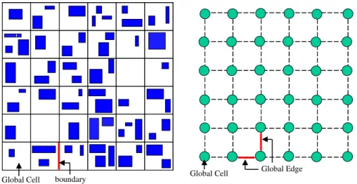
The first step of global routing is to transform a routing region into a routing graph such that routing can be completed on this graph. Figure 1 shows a routing graph model, called grid graph model. The routing space is partitioned into many rectangular grids, called global cells. Then we can model the global routing problem as a routing problem on a grid graph G(V, E), where V and E are the set of nodes and edges of the grid graph. Each node is corresponding to a unique global cell and two nodes have a global edge connecting them if their associated global cells are adjacent, i.e., a global edge is referred to as the boundary of two adjacent global cells in the

Global Cell boundary Global Cell

Global Edge

Fig. 1. (a) The routing space is partitioned into 6×6 global cells. (b) The associated grid graph model of routing space in (a).

original routing space. Besides, every global edge has its own capacity to indicate the maximum number of routing tracks across its corresponding boundary.

2.2 Problem Formulation

Given a global edge e, its capacity is denoted as ce. Assume the total number of

nets passing edge e is de, de is referred to as the demand of edge e. Thus, we can

define the overflow of edge e as the following formula:

The total overflows of a global routing can then be defined as:

Hence, the objective of a global routing problem is to find a routing with minimum total overflow and wire length:

Minimize: tof and

∑

∈E

e e

d .

2.3 The Overview of FastRoute

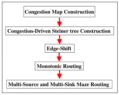
Figure 2 shows the routing flow of FastRoute [13]. FastRoute first constructs congestion map and congestion-driven Steiner tree based on the congestion map. Edge shifting is then employed to shift the movable edges to decrease overflow. Based on the topologies, every two-pin net is routed by monotonic routing. Finally, FastRoute uses multi-source and multi-sink maze routing to rip up and reroute the nets across congested regions. We will introduce each stage in the following sub-sections. (2)    − > = . , 0 , ) ( . otherwise c d if c d e overflow e e e e (1)

∑

∈ = E e e overflow tof ( )

2.3.1 Congestion Map Construction

There are two major methods to estimate the congestion – one is to build a probability formula to estimate the distribution of all nets; the other way is actually routing all nets and collecting the routing information for congestion estimation, FastRoute [13] adopts the latter method. FastRoute applies Flute [11] to generate all tree topologies rapidly. After building the topologies, it completes routing in straight-line or L-shape pattern, with the routing costs 1.0 and 0.5 for two patterns, respectively.

Fig. 2. The routing flow of FastRoute.

Congestion Map Construction

Congestion-Driven Steiner tree Construction Edge-Shift

Monotonic Routing

Multi-Source and Multi-Sink Maze Routing Congestion Map Construction

Congestion-Driven Steiner tree Construction Edge-Shift

Monotonic Routing

2.3.2 Congestion-Driven Steiner Tree Construction

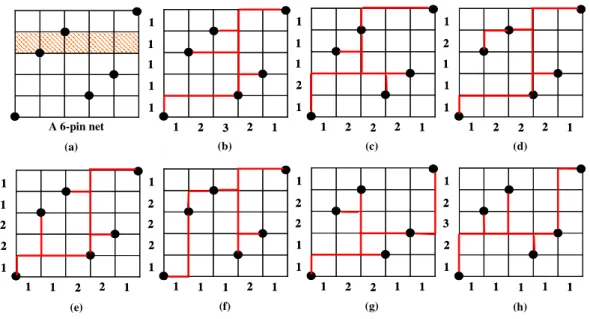
FLUTE [11] builds rectilinear Steiner minimal tree (RSMT) by using a lookup table. A net of degree n can be divided into n! sets based on the relative positions of its pins. The wire length of all topologies can be computed by the linear combination of the distances between adjacent Hanan grid lines. A linear combination can be viewed as a vector of the coefficients, and FLUTE calls this vector as potentially optimal wire length vector (POWV), as shown in Fig. 3. Hence FLUTE can obtain minimum wire-length topology by computing all POWVs and their own corresponding segment distances.

FastRoute utilizes POWV as the amount of usages of the corresponding segments. The topology of in Fig. 3(b) contains more horizontal segments but less vertical segments than that in Fig. 3(h). Since two topologies usually have different using frequencies of segments, FastRoute identifies the routing topology that contains as many segments across less congested regions as possible. For example, in Fig. 3(a), if the second column in the shaded region is congested, FastRoute will yield the topology in Fig. 3 (b) rather than in Fig. 3(c) since the former does not pass through

1 1 2 2 1 1 2 2 1 1 1 1 2 2 1 1 2 2 1 1 1 1 1 2 1 1 2 2 2 1 1 1 1 2 1 1 2 2 2 1 1 2 2 1 1 1 1 2 2 1 1 2 2 1 1 1 1 2 2 1 1 1 1 1 1 1 2 3 2 1 1 1 1 1 1 1 2 3 2 1 1 2 3 2 1 1 1 1 1 1 1 2 3 2 1 1 1 1 1 1 1 2 2 2 1 1 2 1 1 1 1 2 2 2 1 1 2 1 1 1 1 2 2 2 1 1 1 1 2 1 1 2 2 2 1 1 1 1 2 1 A 6-pin net (b) (c) (d) (e) (f) (g) (h) (a)

Fig. 3. Seven possible Steiner-tree topologies of a six-pin net in (a) and their own POWV.

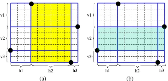
the second column that is congested. To achieve this goal, FastRoute first computes the corresponding congestion cost for each segment. For instance, in Fig. 4(a), the horizontal segment h2 computes the shaded column area as its total congestion cost. This implies that if this column area is congested, h2 segments are not preferable to be involved in the routing topology. Figure 4(b) shows a similar situation for a vertical segment v2. Besides, the average congestion cost of a horizontal/vertical segment is the ratio of total demand to total capacity of all global edges in the corresponding column/row area. The distance of a segment is scaled by its average congestion cost. Then congestion-driven Steiner tree construction problem is transformed into a traditional Rectilinear Steiner Minimal Tree (RSMT) problem weighted using scaled wire-length cost. FLUTE can then be invoked to seek a minimal Steiner tree with balanced wire length and congestion cost.

v1 v2 v3 h1 h2 h3 v1 v2 v3 h1 h2 h3 v1 v2 v3 h1 h2 h3 v1 v2 v3 h1 h2 h3 (a) (b)

Fig. 4. (a) The yellow region is the column area of a horizontal segment h2. (b) The green region is the row area of a vertical segment v2.

2.3.3 Edge-Shifting

After constructing an initial topology, FastRoute applies edge shifting to reduce overflow in advance. Figure 5 displays an example of edge shifting to evade congested regions, where the red edge is a movable edge and the shaded regions are congested regions. Figures 5(b), (c) and (d) display three cases of edge shifting for the movable edge under three scenarios. Note that, the wire length after edge shifting must be kept unchanged. The movable edge has the following characters: (1). both end nodes of this edge is of degree 3; (2). this edge has a safe sliding range for shifting to make sure that the final wire length remains unchanged. If an edge owns the above features, it is called a movable edge. The safe sliding range is showed in Fig. 5(a). For the red movable edge in Fig. 5(a), its left and right end points can be shifted within ranges R1 and R2, respectively. The overlapping range of R1 and R2 is the final safe sliding range of the movable edge. Afterward the total congestions of all possible topologies are computed and the minimum-cost topology is selected to Fig. 5. (a) Original routing tree and its movable edge; (b) un-congested region

is on the bottom and the movable edge is shifted to the bottom; (c) un-congested region is in the middle and the movable edge is shifted to the middle; (d)

un-congested region is on the top and the movable edge is shifted to the top.

R2 R1 R3 (a) (b) (c) (d) R2 R1 R3 (a) (b) (c) (d)

determine the position of the movable edge.

2.3.4 Monotonic Routing

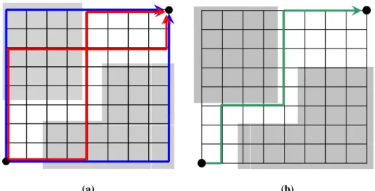
For two-pin net routing, maze routing and pattern routing algorithms are two extreme types of routing algorithms – the former is very slow but can find a minimum-cost path, yet the later is very fast at the cost of low quality or completion rate, as shown in Fig. 6(a). As compared to pattern routing, monotonic routing enlarges the solution space to multiple-bend and detour-free routing paths. Monotonic routing is considerably fast as compared to maze routing. Monotonic routing is also known as dynamic pattern routing. Each global cell is reachable from its one or two neighbors. For instance, in Fig. 6(b), the directions of monotonic routing are rightward and upward, so each global cell is accessible only from its left and bottom neighbors. For each global cell, the neighbor with minimum congestion cost will be selected as its predecessor. There are C(m+n, m) possible monotonic routing solutions for a m×n grids. Figure 6(b) presents an example of monotonic routing to avoid the congested regions. The complete algorithm of monotonic routing in FastRoute is shown in Fig. 7. The time complexity of monotonic routing is O(mn), where m and n

Fig. 6. (a) A routing region that can not be solved using L-shape and Z-shape patterns; (b) Monotonic routing can find an overflow-free routing path.

are the number of horizontal and vertical grids respectively. Its time complexity is the same as that of Z-shape pattern routing, but it enriches its solution space as compared to L-shape and Z-shape routings.

2.3.5 Multi-Source and Multi-Sink Maze Routing

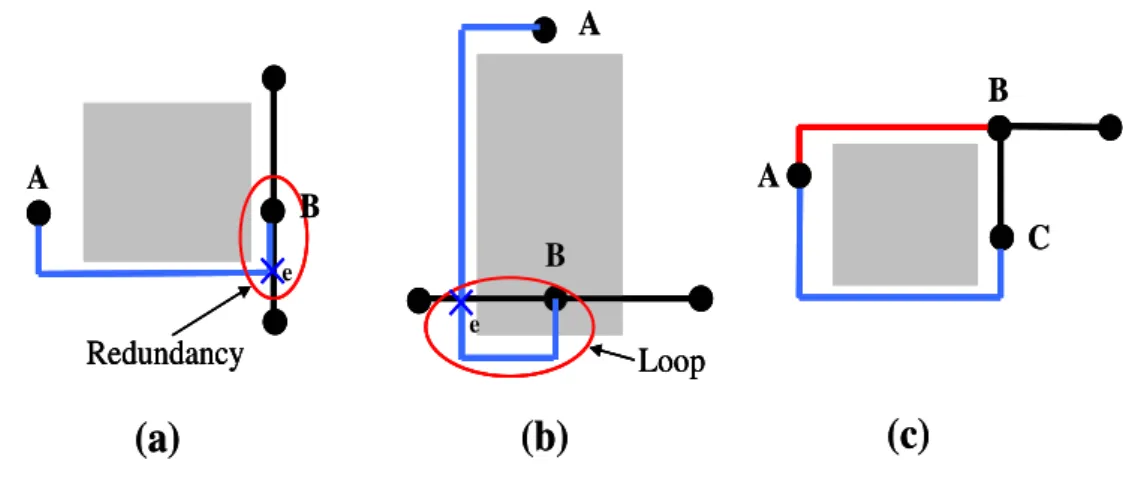
Maze routing is frequently employed to search a point-to-point routing path. However, some problem arises when it is applied in global routing to complete a net routing, that has been split into multiple two-pin net routings. Figure 8 displays these problems, including redundancy, looping and unnecessary detour:

(1). Redundancy : In Fig. 8 (a), the two-pin net routing connects nodes A and B.

Point-to-point maze routing usually yields an overlap segment, for example, eB in Fig. 8(a). Redundant wire results in the increase in wire length as well as congestion.

(2) Loop : Another problem induced by point-to-point maze routing is circular path. In Fig. 8(b), the routing path has connected a point e on the path containing target point B before reaching target B. Finally a loop appears in the routing path of the net.

(3) Unnecessary Detour: In Fig. 8(c), nodes A and C are initially designed to be connected. The blue wire displays the routing result with a detour. Actually, connecting these two disjoint sets has better alternative. The red wire in Fig. 8(c) displays a detour-free L-shape path.

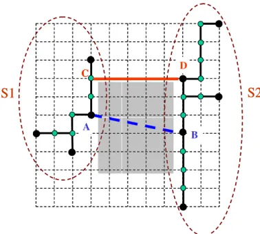
To solve the above problems, FastRoute proposes the multi-source and multi-sink maze routing algorithm. The main idea of this algorithm is to connect two sets of nodes instead of two nodes, i.e., all nodes on the sub-tree containing original start/target node are regarded as start/target nodes. Routing is complete if any one start node connects to any one target node. Figure 9 shows an example of multi-source and multi-sink maze routing, where the blue segment is the path generated by conventional maze routing algorithm, and the red segment connecting

Redundancy _Loop

(a)

(b)

(c)

A B B A A B C Redundancy

Redundancy _LoopLoop

(a)

(b)

(c)

A B B A A B C e e

Fig. 8. Three possible problems induced by point-to-point maze routing. (a) Redundant wire; (b) circular path; (c) unnecessary detour.

nodes C and D is a better result and produced by multi-source and multi-sink maze routing algorithm. A B

S1

C D

S2

A B

S1

C D

S2

Fig. 9. Point-to-point maze routing regards nodes A and B as start and target

nodes respectively. Multi-source and multi-sink maze routing regards all nodes of

two sub-trees as start and target nodes. Nodes C and D are new connection points

Chapter 3

Global Routing Algorithm

Compared with other state-of-the-art global routers, FastRoute [13] is extremely fast. Because maze routing is very time-consuming, FastRoute diminishes overflow as much as possible before entering maze routing stage. In this thesis, we refine edge shifting and node shifting technique to alter the topology of Steiner tree for decreasing overflow in advance. Besides, we propose mirrored monotonic routing technique to lower the usage of maze routing for saving routing time.

3.1 Edge Shifting Refinement

3.1.1 Movable Edges

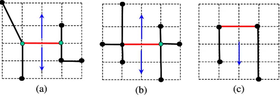
FastRoute only shifts the edge whose both end points are of degree 3 and keeps the wire length unchanged. Actually, shifting an edge with a degree-4 Steiner node and a degree-2 pin node can also reduce overflow without changing wire length. For example, Fig. 10(a) represents a movable edge identified in FastRoute. Figures 10 (b) and (c) display two movable edges with endpoints of degrees 4 and 2 respectively.

In Fig. 10(c), if the movable edge is shifted upwards, the wire length will increase, so in our method we do not move it upward. Thus, our proposed edge shifting guarantees to keep wire length unchanged.

3.1.2 Routing Tree Selection

Traditionally, the routing tree with minimum congestion is selected out of the routing trees derived by edge shifting. According this selection rule, an overflow-free routing tree with high total demand will not be selected as final solution. In this work, we attempt to balance the minimization between overflow and congestion by refining the cost function for routing-tree selection as follows:

(a) (b) (c) (a) (b) (c)

Fig. 10. Movable edges in FastRoute and our global router. The black and green nodes are the pins of the net and the Steiner points. (a) A movable edge defined in FastRoute; (b) a movable edge with endpoints of degree 4 in our global router; (c) a movable edge with endpoints of degree 2 in our global router.

( )

T overflow

( )

T congestion

( )

T t =

α

∗ +

β

∗

where α and β are coefficients, T is the routing tree for selection, overflow(T) is the overflow amount of T, and congestion(T) is its total congestion. In this work, overflow minimization is our main objective, so the overflow factor is adjusted to dominate this function.

3.2 Node Shifting

Edge shifting is a successful technique in routing tree restructuring for overflow reduction. Another available routing tree restructuring technique for overflow reduction is node shifting. Node shifting has been employed in restructuring rectilinear Steiner tree [15]. We also apply this technique for seeking an overflow-free routing tree. A C B D S a b c d e A C B D S a b c d e A C B D S A C B D S A C B D S A C B D S (a) B A C D S (b) B A C D S (b) A C D S (b) (c) (d)

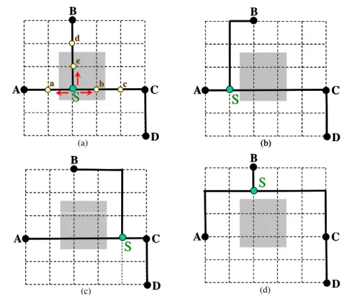
Fig. 11. (a) Five possible points, a, b, c, d, and e for node shifting on Steiner point S. Points a, c, and d can decrease overflow; (b) overflow is decreased by shifting

Steiner point S to point a; (c) overflow is decreased by shifting Steiner point S to

Figure 11(a) shows a routing tree with a Steiner point S inside a congested region. In this case, edge shifting is helpless in removing overflow but node shifting can solve the problem. For Steiner point S, points a, b, c, d, and e are its possible target points. Points b and e are inside congested region (shaded region in the figure), so they are not considered as target points. Figures 11(b) , (c) and (d) displays the results of shifting S to a, c and d, respectively. Only point d can produce an overflow-free routing tree. Note that we only shift a Steiner point of degree 3 in congested region. A Steiner point of degree 4 is not considered as a shifted node since shifting a node of degree 4 in any one direction always leave one edge in congested region, as shown in Fig. 12.

Node shifting enriches the flexibility of routing tree restructuring to exploit an overflow-free routing tree. Its disadvantage is the increase in wire length.

3.3 Mirrored Monotonic Routing

FastRoute performs time-consuming maze routing following monotonic routing to seek an alternative path. To increase routing speed, we propose a refined monotonic routing technique, called mirrored monotonic routing, to replace maze routing for some routings producing only one detour.

S

a b c d

S

a b c d

Kahng et al. [16] proposed an area expansion method to iteratively estimate the wire length of a detoured net for a placement. Inspired by the area expansion method, we enlarge the bounding box of a two-pin net routing by copying the column containing target point and putting it to the opposite side of the column next to the target column. This process is called target mirroring. Monotonic routing is then employed on the new routing region to seek a routing path and the target point in the

B’ X B A X X+1 (d) B’ X B A X X+1 B’ X B A X X+1 (d) B’ X B A X X+1 (e) B’ X B A X X+1 B’ X B A X X+1 B’ X B A X X+1 (e)

Fig. 13. An example of mirrored monotonic routing. (a) Monotonic routing can

not seek an overflow-free path; (b) an overflow-free path with one detour; (c) copy

column x to the right of column x+1 (mirror operation) ; (d) apply monotonic

routing on the expanded routing region with additional one mirrored column; (e)

mirror the routing path found by monotonic routing to yield a one-detour

overflow-free routing path.

A B (a) A B A B (a) A B (b) ₁ A B (b) A B A B A B (b) ₁ Congested region B B’ A X X+1 X (c) B B’ A X X+1 X (c) B B’ A X X+1 X B B’ A X X+1 X B B’ A X X+1 X (c)

additional mirrored column is the new target point. Figure 13 (a) shows that monotonic routing can not identify an overflow-free path, where a shaded region is referred to as a congested region. Figure 13(b) displays that the shortest path without overflow has one detour. Figure 13(c) shows a mirroring operation. If an overflow-free routing path is identified, the partial segments in the mirrored column have to be restored to the original target column through mirroring again, as shown in Fig. 13(d). The advantage of this approach is to fast yield a one-detour overflow-free routing path. However, the number of this type of routing paths in a routing problem determines the profit we can gain from this approach.

3.4 The Flow of Our Global Router

Figure 14 displays the routing flow of our global router. Our original routing flow is based on the routing flow of FastRoute; besides, we introduce the negotiation-based technique in [17] to the multi-source and multi-sink maze routing stage. Node shifting is performed following refined edge shifting. Before employing

Fig. 14. Proposed global router’s flow. Congestion Map Construction

Congestion-Driven Steiner tree Construction

MirroredMonotonic Routing

Multi-Source and Multi-Sink Maze Routing

Extended Edge-Shift

Node-Shift

Monotonic Routing Congestion Map Construction

Congestion-Driven Steiner tree Construction

MirroredMonotonic Routing

Multi-Source and Multi-Sink Maze Routing

Extended Edge-Shift

Node-Shift

maze routing to solve congested routings, mirrored monotonic routing is invoked to seek some one-detour routing patterns.

Chapter 4

Experimental Results

We implement the proposed global router in C++ programming language, and perform experiments on a computer with AMD Opteron 2.0GHz CPU ,16GB memory and Linux operating system.

Two sets of benchmark circuits are used in this thesis. One set is ISPD98 benchmarks [18], and the other set is ISPD07 benchmarks [19].

4.1 ISPD98 Benchmarks

Table 1 lists the statistics of ISPD98 benchmarks. Since the proposed two routing techniques are employed before maze routing, we compare the routing results before maze routing with and without applying these two routing techniques to show the quality improvement. In Table 2, columns 3, 4 and 5 list the routing results obtained by applying refined edge shifting, node shifting and both techniques, respectively. Every row (design) has two data. The data without and with mirrored monotonic routing are listed in the top and bottom rows, respectively. Refined edge shifting and node shifting are 5.9% and 4.7% more effective in decreasing overflow than FastRoute. Both techniques offer more 13% overflow reduction rate than FastRoute. For runtime, refined edge shifting, node shifting, and both techniques all can speed up the routing by 33%, 36%, and 38% respectively.

In Table 3, we compare our total overflow, wire length and runtime with three state-of-the-art global routers – FastRoute 2.0, BoxRouter, and Labyrinth. Our router does not yield any overflow in all cases and achieves about 3.6X and 15.5X faster than BoxRouter and Labyrinth, but still runs 4.3X slower than FastRoute.

Benchmark Grids #Nets #Routed Nets ibm01 64x64 11.5k 9.1k ibm02 80x64 18.4k 14.3k ibm03 80x64 21.6k 15.3k ibm04 96x64 26.2k 19.7k ibm06 128x64 33.4k 25.8k ibm07 192x64 44.4k 34.4k ibm08 192x64 47.9k 35.2k ibm09 256x64 50.4k 39.6k ibm10 256x64 64.2k 49.5k

Table 2. The effect of extended edge-shift, node-shift, and mirrored monotonic routing.

(*)Overflow before maze routing stage.

Original Flow with Edge-Shift Ext. with Node-Shift With Both Techniques

Of/bm* Time(s) Of/bm* Time(s) Of/bm* Time(s) Of/bm* Time(s)

w/o MMR 1674 6.86 1689 7.45 1539 4.84 ibm01 with MMR 1730 10.42 1438 6.4 1507 6.01 1297 3.6 w/o MMR 4123 5.49 4126 7.36 3883 4.7 ibm02 with MMR 4281 14.47 3075 6 3212 6.91 2798 5.2 w/o MMR 705 1.46 746 1.30 650 1.27 ibm03 with MMR 779 2.45 543 1.91 539 1.33 458 1.82 w/o MMR 2733 63.63 2808 53.58 2585 57.5 ibm04 with MMR 2936 72.03 2079 54.54 2449 45.81 1980 43.54 w/o MMR 3574 5.41 3646 6.54 3426 5.38 ibm06 with MMR 3849 13.36 2771 5.62 2683 5.36 2484 5.88 w/o MMR 2673 5.49 2725 5.84 2467 5.34 ibm07 with MMR 2859 9.96 2210 6.77 2274 6.05 2042 5.9 w/o MMR 3840 7.67 3832 6.62 3502 8.12 ibm08 with MMR 4205 14.16 3048 6.93 3354 8.96 2779 7.78 w/o MMR 4297 5.81 4439 8.14 3951 5.75 ibm09 with MMR 4564 11.43 3322 7.05 3651 6.74 3185 6.41 w/o MMR 6824 13.36 6791 13.48 6527 12.83 ibm10 with MMR 7033 23.96 5973 14.32 5996 15.87 5697 14.6 w/o MMR 30443 115.18 30802 110.31 28530 105.73 Total with MMR 32236 172.24 24459 109.54 25665 103.04 22720 94.43

4.2 ISPD07 Benchmarks

Table 4 shows the statistics of 2-D benchmarks in ISPD07 Global Routing Contest. These benchmarks are larger than ISPD98 benchmarks, and they have 2-D and 3-D versions. In this work, we only consider the 2-D routing. Table 5 compares our routing results with FGR, MaizeRouter, BoxRouter, and FastRoute presented in this contest [20]. Our global router yields the worst wire length in all cases, the worst total overflow in newblue1, and the third total overflow in newblue3. The proposed refined edge shifting allows increasing the wire length of a routing tree, so the wire length of our results is getting worse.

Table 3. Comparison of our global router( New and Original flow), FastRoute 2.0, BoxRouter, and Labyrinth.

New Flow Original Flow FastRoute2.0 BoxRouter Labyrinth

tof twl time(s)tof twl time(s)tof twl time(s)tof twl time(s) tof twl time(s) ibm01 0 66575 3.59 0 67605 10.42 31 68489 1.08102 65588 7.333 398 76517 24.28 ibm02 0 176964 4.92 0 175138 14.47 0 178868 1.4 33 178759 25.23 492 204734 42.23 ibm03 0 148161 1.27 0 148175 2.45 0 150393 0.9 0 151299 14.32 209 185116 41.4 ibm04 0 174357 41.69 0 174264 72.03 64 175037 2.82309 173289 19.054 882 196920 110.16 ibm06 0 286760 5.88 0 284218 13.36 0 284935 2.04 0 282325 26.93 834 346137 88.77 ibm07 0 375000 4.83 0 374885 9.96 0 375185 2.4 53 378876 40.175 697 449213 198.7 ibm08 0 415299 7.66 0 413497 14.16 0 411703 3.54 0 415025 67.93 665 469666 213.65 ibm09 0 420917 7.29 0 421378 11.43 3 424949 2.88 0 418615 50.99 505 481176 301.8 ibm10 0 600023 14.6 0 594691 23.96 0 595622 4.19 0 593186 75.303 588 679606 397.07 total 02664056 91.73 02653311172.24 982665181 21.254972656962 327.2752703089085 1418.1 norm 1 1 0.99 1.88 1.00042 0.232 0.99734 3.568 1.15954 15.460

Table 5. Comparison of our global router, FGR, MaizeRouter, BoxRouter, and FastRoute. Benchmark name Grids #Nets

Adaptec1 324x324 219794 Adaptec2 424x424 260159 Adaptec3 774x779 466295 Adaptec4 774x779 515304 Adaptec5 465x468 867441 Newblue1 399x399 331663 Newblue2 557x463 463213 Newblue3 973x1256 551667

Table 4. The statistics of ISPD07 benchmarks.

New Flow Original Flow FGR MaizeRouter BoxRouter FastRoute

twl tof Time(m) twl tof Time (m)

twl tof twl tof twl tof twl tof

a1 86.59 0 104.8 85.89 0 129.12 55.80 0 62.26 0 58.84 0 90.47 122 a2 79.10 0 420.4 79.00 0 533.6 53.69 0 57.23 0 55.69 0 82.46 500 a3 190.97 0 57.5 190.22 0 60.23 133.3 0 137.75 0 140.8 0 202.53 0 a4 166.69 0 8.9 165.37 0 11.28 126.0 0 128.45 0 128.7 0 170.80 0 a5 250.01 0 652.7 254.63 0 449.9 155.8 0 176.69 2 164.3 0 251.68 9680 n1 73.57 2212 270.6 73.10 2206 369.4 47.51 1218 50.93 1348 51.13 400 74.10 1934 n2 112.69 0 2.0 110.05 0 2.93 77.67 0 79.64 0 79.78 0 114.95 0 n3 159.04 36172 301.0 158.07 36098 285.73 108.2 36970 114.63 32588 111.6 38976 154.59 34236

Chapter 5

Conclusions

In this thesis, we propose two routing techniques – refined edge shifting and mirrored monotonic routing. The former increases the possibility to lower overflow using edge shifting technique while the later utilizes monotonic routing to replace maze routing in some one-detour routing patterns. Experimental results reveal that the proposed approaches enhance the routability and speed of our global router before entering maze routing stage. Unfortunately, node shifting probably increases the wire length of a routing tree. Experimental results on ISPD07 benchmark circuits also show this defect. Node shifting with wire length constraint will be studied further.

Chapter 6

Bibliography

[1] J. Lou, S. Krishnamoorthy, and H. Sheng. Estimating routing congestion using probabilistic analysis. In Proc. Intl. Symp on Physical Design, pp. 112-117, 2001. [2] A. Kahng and X. Xu. Accurate pseudo-constructive wirelength and congestion estimation. In Proc. Intl. Workshop on System-Level Interconnect Prediction(SLIP), pp. 61-68, 2003.

[3] R. Hadsell and P. Madden. Improved global routing through congestion estimation. In Proc. ACM/IEEE Design Automation Conf., pp. 28-31, 2003.

[4] J. Westra, C. Bartels, and P. Groeneveld. Probabilistic congestion prediction. In Proc. Intl. Symp on Physical Design, pp. 204-209, 2004.

[5] C. Sham and E. Young. Congestion Prediction in Early Stages. In Proc. System-Level Interconnect Prediction, April 2005.

[6] R. Kastner, E. Bozogzadeh, and M. Sarrafzadeh. Predicable routing. In Proc. IEEE/ACM Intl. Conf. Computer-Aided Design, pp. 110-113, 2006.

[7] J. Kruskal. On the shortest spanning subtree of a graph. Proc. American Math Society, 7:48-50,1956.

[8] Shortest connecting networks. Bell System Technical Journal, 31:1398-1401,1957. [9] E. Bozorgzadeh, R. Kastner, M. Sarrafzadeh. Creating and exploiting flexibility in rectilinear Steiner trees. In : Computer-Aided Design of Integrated Circuits and Systems, IEEE Transactions, pp. 605-615, 2003.

[10] M. Cho, D. Pan. BoxRouter: A New Global Router Based on Box Expansion and Progressive ILP. In Proc. Design Automation Conf., pp. 373-378, 2006.

Proc. Int. Conf. on Computer Aided Design, pp. 696-701, 2004.

[12] M. Pan, C. Chu. FastRoute: A Step to Integrate Global Routing into Placement. To appear. IEEE/ACM Intl. Conf. Computer-Aided Design, 2006.

[13] M. Pan, C. Chu. FastRoute 2.0: A High-quality and Efficient Global Router. In Asia and South-Pacific Design Automation Conference, pp.250-255, 2007.

[14] Z. Cao, T. Jing, J. Xiong, Y. Hu, L. He, X. Hong. DpRouter: A Fast and Accurate Dynamic-Pattern-Based Global Routing Algorithm. In Asia and South-Pacific Design Automation Conference, pp. 256-261, 2007.

[15] D. Pan, Architecture and Implementation of a Robust Global Router for Ultimate Routability. In IEEE/ACM Intl. Conf. Computer-Aided Design, 2007.

[16] A. Kahng ,X. Xu. Accurate pseudo-constructive wirelength and congestion estimation. In Proc. Intl. Workshop on System-Level Interconnect Prediction(SLIP), pp. 61-68, 2003.

[17] L. McMurchie ,C. Ebeling, “PathFinder: A Negotiation-based Performance-driven Router for FPGAs,” In Proc. ACM Symp. on FP-GAs, 1995. [18] http://www.ece.ucsb.edu/~kastner/labyrinth/benchmarks/

[19]http://www.sigda.org/ispd2007/contest.html [20] http://www.ispd.cc/slides07/gr-contest.pdf