國
立
交
通
大
學
電 子 工 程 系
碩
士
論
文
數位射頻干擾消除技術應用於
超高速數位用戶迴路系統
Digital RFI Cancellation in DMT-based VDSL systems
研 究 生:江啟仁
指導教授:桑梓賢 教授
數位射頻干擾消除技術應用於
超高速數位用戶迴路系統
Digital RFI Cancellation in DMT-based VDSL systems
研 究 生:江 啟 仁 Student:Chiang Chi-Jen 指導教授:桑 梓 賢 Advisor:Sang Tzu-Hsien 國 立 交 通 大 學 電 子 工 程 學 系 碩 士 論 文 A Thesis
Submitted to Department of Electronics Engineering College of Electrical Engineering and Computer Science
National Chiao Tung University in partial Fulfillment of the Requirements
for the Degree of Master
in
Electronics Engineering
June 2005
Hsinchu, Taiwan, Republic of Chin
數位射頻干擾消除技術應用於
超高速數位用戶迴路系統
研究生: 江啟仁 指導教授: 桑梓賢 博士 國立交通大學 電子工程學系 電子研究所碩士班 摘要 VDSL 是利用大眾電話網路提供寬頻接取的服務。衍生出來的問題是此電話 網路是使用無遮蔽效果的雙絞線,而且 VDSL 這項技術又與業餘無線電及 AM 廣播電台共享頻帶,如果在電話線路附近有一無線電發射端,則射頻訊 號將會進入無遮蔽效果的雙絞線產生干擾,這種現象稱為射頻干擾(Radio Frequency Interference)。一般而言,業餘無線電對 VDSL 的訊號產生的干擾 比 AM 廣播電台還嚴重,因此論文內容著重於處理業餘無線電對 VDSL 產 生的干擾。關於 RFI 演算法的模型,最簡單的模型是假設每個 Zipper VDSL 字符時間中的 RFI 波封為常數[9]。但是在 ETSI VDSL 的系統中,每個字符 時間比 Zipper VDSL 長數倍,所以 RFI 波封有時後並不為常數,因此使用 此模型並不完全準確。我們提出一個較為準確的 RFI 演算法的模型來達到 消除 RFI 的目地。模擬的結果可以證明我們演算法是可以有效消除 RFI。Digital RFI Cancellation in DMT-based VDSL systems
研 究 生:江啟仁 student:Chi-Jen Chiang
指導教授:桑梓賢 Advisors:Tzu-Hsien Sang
Department of Electronics Engineering National Chiao Tung University
ABSTRACT
VDSL is a promising technology of unshielded twisted pairs in the public telephone network for the purpose of broadband access. A problem with this technology is that the frequency range used for VDSL signaling is shared with amateur radios and broadcast AM radios. A transmitter in the proximity of a wire will induce an electrical signal in the wire; this is called Radio Frequency Interference (RFI).
In general, amateur radio (HAM) is more harmful than AM in VDSL. In this paper, we will focus on dealing with amateur radio. In regard to RFI model, the simplest model is zero-order with a constant RFI envelope in one Zipper VDSL symbol period [9]. But in ETSI VDSL systems, the symbol periods are several times longer than that of Zipper VDSL. The RFI envelop in one symbol may not be constant. Therefore, the use of such a model in digital RFI cancellation is not fully justified. We started with a more accurate RFI model and developed an improved way for RFI cancellation. Simulation results show support to our assumptions and the effectiveness of our algorithm.
Contents
中文摘要………..I ABSTRACT………...II ACKNOWLEDGE CONTENT………..III LIST OF TABLES………V LIST OF FIGURES………...V Chapter 1 ... 1 Introduction ... 11.1 Discrete Multi-Tone (DMT) Modulation... 2
1.2 VDSL Deployment configuration ... 4
1.3 VDSL Transmission Environment ... 6
1.4 Thesis Outline ... 10
Chapter 2 ... 11
Radio Frequency Interference ... 11
2.1 AM broadcast radio ... 11
2.2 Amateur radio ... 14
Chapter 3 ... 19
Cancellation Of RFI ... 19
3.1 Requirements of RFI Suppression ... 22
3.2 Jeong and Yoo’s Approach for Parameter Estimation [9] ... 23
3.3 A Digital RFI canceller by Wise and Bingham [10] ... 24
3.4 A Iterative RFI canceller by Huang [7] ... 26
3.5 An RFI Signal Model (Model 1) ... 28
3.5.1 RFI detection and parameter estimation ... 30
3.5.2 Measurement tones selection ... 32
3.6 First order model (Model 2) ... 35
3.7 Reduce computation cost of RFI cancellation algorithm... 38
Chapter 4 ... 40
Chapter 5 ... 43
Simulations... 43
5.1 Single RFI simulation ... 44
5.2 Multiple RFI simulation ... 47
Chapter 6 ... 52 Conclusion... 52 Future Work... 53 Appendix A. ... 59 Appendix B. ... 60 Appendix C. ... 61 Reference... 63
LIST OF TABLES
Table 1.2 VDSL Data rates... 5
Table 2.1-1 signal strengths for AM radio noise into VDSL ... 12
Table 2.1-2 The AM radio noise models for VDSL... 12
Table 2.2 Amateur Radio Bands defined by ANSI ... 15
LIST OF FIGURES Figure 1.2 VDSL Deployment Configuration... 6
Figure 1.3-1 VDSL Near-End crosstalk ... 7
Figure 1.3-2 VDSL Far-End crosstalk ... 7
Figure 1.3-3 VDSL Deployment Configuration alien crosstalk ... 8
Figure 1.3-4An example of RFI ingress... 8
Figure 1.3-5 An example of RFI egress ... 9
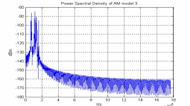
Figure 2.1-1. The Power Spectrum Density of AM model 3 simulation... 13
Figure 2.1-2 The magnification of 2.1-1 in the part of RFI peak ... 14
Figure 2.2-1. Simulation block diagram of amateur radio... 16
Figure 2.2-2 The Power Spectrum Density of RFI simulation ... 16
Figure 2.2-3 Amateur radio vs AM model 3 PSD ... 17
Figure 2.2-4 The PSD level of RFI vs Received signal ... 17
Figure 3-2. RFI in one DMT symbol period ... 21
Figure 3.1-1 The required level of RFI cancellation... 22
Figure 3.5-1 Illustration for the cases ... 31
Figure 3.5-3 Theoretical RFI model (3.5-5) cancellation ... 33
Figure 3.5-4 Simplify RFI model (3.5-6) cancellation ... 34
Figure 3.7 The flow chart of RFI cancellation algorithm ... 39
Figure 5 Compare with PSD for various noise ... 44
Figure 5.1-1 RFI signal suppression by Model 1 algorithm ... 45
Figure 5.1-2 RFI signal suppression by Model 2 algorithm ... 47
Figure 5.2-1 Multiple RFI signal suppression by Model 1 algorithm ... 48
Figure 5.2-2 Multiple RFI signal suppression by Model 1 algorithm ... 51
Figure 6-2 RFI signal suppression by time domain cancellation algorithm ... 56
Figure 6-3 RFI signal suppression by time domain cancellation algorithm ... 57
Chapter 1
Introduction
There are two different modulation schemes in the VDSL standard, i.e. a single carrier modulation scheme using CAP (carrier-less amplitude phase modulation) or QAM (quadrature amplitude modulation), and a multicarrier modulation scheme using the DMT modulation. In this thesis we will focus on a digital RFI cancellation in DMT-based VDSL transmission systems. The VDSL system uses the telephone network (unshielded twisted copper wires) for high-speed digital communication. A problem with this technique is that the frequency range used for VDSL signaling is shared with radio amateurs and broadcast AM radio. The unshielded copper wire acts like a common mode antenna that both radiates and receives energy form radio signal. This will cause two types of RFI which ingresses and egresses [1]. In this thesis we will focus on dealing with the problem of RFI ingress in VDSL system.
The main source of RFI is considered to be the amateur radio transmitters. This is because they can be located just a few meters form unshielded telephone wires. Moreover, the high transmitted power of the amateur radio can cause a great interference in VDSL system. There are two ways of RFI cancellation, analog and digital. A front-end analog cancellation can prevent RFI signal causing clipping in ADC. In order to prevent received signal clipping in ADC, at least 25 dB of cancellation in the analog domain is needed [2]. The analog method can suppress the RFI but often not enough. Usually the digital method operates in the frequency domain after the FFT. In this thesis we will focus on
algorithms which can achieve the RFI cancellation in the digital domain. With the measurement of the RFI on unused tones and a proper RFI model, we are able to evaluate the contribution of RFI on each tone. Then we can subtract the estimated RFI signal from the received signal in frequency domain. Besides, the algorithm can deal with multiple RFIs in a HAM-band. Simulation results show that the algorithm can achieve 40dB RFI cancellation at best.
1.1 Discrete Multi-Tone (DMT) Modulation
Discrete Multi-Tone modulation is the basis of the multi-carrier version of
VDSL. This type of modulation is essentially equivalent Orthogonal Frequency Division Multiplexing (OFDM). The basic concept of DMT is to split a serial high data rate stream into parallel lower data rate streams that are transmitted simultaneously over a number of sub-carriers. Because the symbol duration increases for the lower data rate parallel sub-carriers, the relative amount of dispersion in time caused by multipath delay spread is decreased. Figure 1.1-1 depicts a simplified DMT transceiver used for ADSL and VDSL. The data is first coded using a Reed-Solomon code. After interleaving the coded bytes, the data is modulated using a DMT modulation scheme. In the transmitter, we assume that
{
X 0, , . . . ,X 1 X N / 2 - 1}
(N/2: number of sub-tones) are transmitted complex number data. DMT modulation can be performed by an IDFT which can be implemented very efficiently as an IFFT. The sequence{
X 0, , . . . ,X 1 X N / 2 - 1}
can be considered as frequency domain signals andcan be transmitted in a real world, we must expand the sequence to
{ }
{ }
{
*}
N /2-1 1
0 1 N /2-1 0
R e X , ,...,X X ,Im X ,X ,...,X* for the input of the N-point
IFFT. After the N-point IFFT, the cyclic prefix (CP) is added to the DMT symbol to mitigate the inter symbol interference (ISI) effect.
L
p points CP isadded to original series
{
x0, ,...,x1 xN -1}
. And a new seriesN - N -1 0 1 N -1 p ro p er sym b o l p o in ts cyclic p refix ,...., , , ,..., p p L L
x x x x x is obtained. Notice that
L
p points must beat least equal to or larger than the length of channel impulse response to prevent ISI. Besides, adding CP makes linear convolution equivalent to circular convolution. Circular convolution in time domain is equivalent to tone-by-tone multiplication in frequency domain.
in time domain :circular convolution
in frequency domain
n n n k k ky
h
x
Y
H
X
=
⊗
⊗
⇒
=
⋅
At the receiver, the channel output signal is first shaping-filtered and converted to digital from by an analog-digital converter (ADC). If the channel delay spread is larger than CP, the ISI can no longer be confined without affecting the proper symbol. On way to deal with this issue is to introduce a FIR TEQ filter which can shorten the overall equivalent channel length. Then, we received the time domain signals
y
n and firstL
p points must be removed. Accordingly in thereceiver an FFT module can serve as a demodulation. A frequency equalizer (FEQ) is uesd to estimate i.e., the complex gain caused by channel. And this
can be achieved by using training sequences during the training phase before a communication link is established. After estimating the channel effect on each tone, we can further estimate the SNR. In a wire-line system such as DSL, the
k
channel capacity can be fully utilized. It means that sub-carriers with high SNRs should be assigned with more data bits, and less data bits are carried in those with lower SNRs. This procedure is called bit loading. Finally, the signals are decoded and the original transmitted data can be recovered.
Figure 1.1 A DMT-based DSL system
1.2 VDSL Deployment configuration
The VDSL systems operates over the copper wires in much the same way
high data rates up to 52 Mbps downstream and 6.4 Mbps upstream. However, the price paid for the higher speed is the shortened distance range. Due to the large attenuation of high-frequency signals on twisted-pair lines, the deployment of VDSL is limited to a loop length of less than 4500ft (1.5Km) form the signal source. Table 1.2 depicts the VDSL data rates in different loop lengths.
Asymmetric Services Data Rate Symmetric Services Data Rate Loop Length Classification Downstream Mb/s Upstream Mb/s Each Direction Mb/s Short Loop (1500 ft) 52 6.4 26 Medium Loop (3000 ft) 26 3.2 13 Long Loop (4500 ft) 6.5 0.8 6.5
Table 1.2 VDSL Data rates [12]
Figure 1.2 shows two possible VDSL deployment configuration, which can deal with limited range of transmission loop length. For customers close to the central office (CO), VDSL can be deployed over copper wiring from CO; this configuration is called fiber to the exchange (FTTEx). For more-distant customers the fiber is run to an optical network unit (ONU). This configuration is called fiber to the cabinet (FTTCab).
VTU-R: VDSL Transmission Unit at the remote customer site VTU-O: VTU at ONU
AN: access network NT: network termination
Figure 1.2 VDSL Deployment Configuration [14]
1.3 VDSL Transmission Environment
The DSL technological advances have increased the potential capacity of the
telephone operators’ access networks, which were originally intended only to provide a plain old telephone service (POTS). The performance of VDSL is not only limited by signal degradation but also by different noises occur on the telephone lines. The most common noises include crosstalk, radio frequency interference (RFI), impulse noise and background noise.
1. Crosstalk
Crosstalk occurs when electromagnetic radiation in a wire affects another wire in the same cable. Such coupling increases with frequency. There are two different types of crosstalk in multi-pair access network cables, near-end crosstalk (NEXT) and far-end crosstalk (FEXT), as show in Figure1.3-1and
1.3-2. NEXT is caused by signals traveling in the opposite direction. FEXT is caused by signals traveling in the same direction. NEXT increases with 1.5
f
and FEXT increases with 2 2
( , )
H f L ⋅ ⋅L f where L is length of the line, is frequency, and
f
( , )
H f L is the magnitude of loop insertion gain transfer
function. NEXT is usually more harmful than FEXT because NEXT is not attenuated by the transfer function. Higher transmitted frequency in VDSL usually means larger crosstalk. Because VDSL signals use bandwidth up to 12MHz, these noise can be very large, especially if the crosstalk signal is another VDSL signal at the same time and frequency. Crosstalk (NEXT and FEXT) can be caused by VDSL signals themselves, in which case we call them self-crosstalk (S-NEXT and S-FEXT), or by other disturbers (e.g. other kinds of DSL signals), in which case we call them alien crosstalk (A-NEXT and A-FEXT), as show in Figure 1.3-3.
Figure 1.3-1 VDSL Near-End crosstalk
Receiver FEXT Cable Wire pair Wire pair Transmitter
Figure 1.3-3 VDSL Deployment Configuration alien crosstalk [14]
2. Radio frequency interference (RFI)
RFI noise is caused by AM or amateur radio (HAM) signal that is transmitted in close proximity of a VDSL transceiver. There are two types of RFI which ingresses and egresses as shown in Figure 1.3-4 and 1.3-5.
Figure 1.3-5 An example of RFI egress [12]
The most straightforward method of reducing RF egress and ingress is to use shielded cable for all aerial sections, but it is probably the most expensive method. For more details, please refer to Chapter 2.
3. Impulse noise
Impulse noise is a temporary signal that can be narrowband or wideband and occurs randomly. Impulse noise can be caused by a variety of electronic and electromechanical devices, and also by atmosphere electrical surges. Impulses can be tens of millivolts in amplitude and can last as long as hundreds of microseconds. Therefore, the VDSL transceivers use forward error correcting codes and interleaving to provide protection against impulse noise.
4. Background noise
This noise is additive white Gaussian noise (AWGN) with fixed power spectral density (PSD) level of -140 dBm/Hz defined in [3]. This level usually corresponds to the reference noise floor.
1.4 Thesis Outline
In Chapter 2, we will introduce the situation that RFI signals interfere with VDSL systems and properties of RFI signals. In Chapter 3 we will indicate the difference in previous RFI cancellation algorithms and propose a new RFI cancellation algorithm. Multiple RFI cancellation is discussed in Chapter 4. The simulation results are showed in Chapter 5.
Chapter 2
Radio Frequency Interference
VDSL systems should avoid interfering existing services, at the same time mitigate impairments caused by other services; emission from VDSL should be controlled the transmitted PSD level in these radio frequency bands no higher than -81dBm/Hz [1]. To prevent ingress, there are tow major ways to mitigate the problem of RFI, analog and digital. An analog cancellation can prevent received signal clipping in ADC and at least 25 dB of cancellation in the analog domain is needed [2]. The analog method can suppress the RFI but often not enough. The digital method mostly operates in the frequency domain after the FFT. In this thesis we will focus on an algorithm that achieves the RFI cancellation in the digital domain.
The VDSL standard specifies that the RFI tests shall be performed while subject to simulated RFI threats as specified in Section 2.1 and 2.2. Each simulated RFI threat shall include 10 simulated AM broadcast stations in the band 535 to 1605 kHz and one amateur radio SSB transmission [3].
2.1 AM broadcast radio
Broadcast AM radio is operated to use the frequency band from 535 to 1605
kHz which overlaps VDSL band. The transmitter may use very high power up to 50KW PEP (Peek Envelope Power). So this powerful RF-transmitter can cause a very large RFI at the neighborhood of Digital subscriber Line. But at a
sufficiently large distance the RFI will be small enough to be handled. There are three model of AM radio noise in Table 1 [3]. Model 1 and Model 2 represent urban high-density areas, and Model 3 represents a suburban environment. The following differential mode levels are based on measurements.
(CM = common mode; DM = differential mode)
Table 2.1-1 signal strengths for AM radio noise into VDSL [3]
Table 2.1-2 The AM radio noise models for VDSL [3]
NOTE 1:
CM is a longitudinal signal with the common mode terminated in 50 Ohm. DM is a differential signal with the differential mode terminated in 100 Ohm.
Model 1 has 2 AM stations at 300 ft, 2 more at 6000 ft , 4 more at 12000 ft, and 2 at 24000 ft.
Model 2 has 1 AM stations at 300 ft, 5 more at 6000 ft.(with 2 at the slightly higher level of -50 dBm) , 3 at 12000 ft, and 1 at 24000 ft.
Model 3 has 5 at 6000 ft. (two are slightly higher at -50 dBm), 3 at 12000 ft, and 2 at 24000 ft.
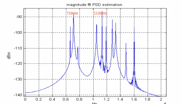
1130kHz 710kHz
Figure 2.1-2 The magnification of 2.1-1 in the part of RFI peak (10 RFI peaks indicate 10 AM broadcast stations)
2.2 Amateur radio
Amateur radio users (HAM) can be harmful because they can be located just a few meters from unshielded telephone wire, and the transmitting power in European is usually below 400W PEP (Peek Envelope Power) while it can be as high as 1500W in the US. Amateur radio users are allowed to use several different frequency bands, calls HAM bands, in the range 1.81MHz~30MHz. The international HAM bands are listed in Table 2.2 [3]. The VDSL spectrum varies with number of sub-carriers N’. There are 2 operating modes: N’=2048 and N’=4096, the sub-carriers spacing ∆ =f 4.3125KHz. The VDSL uses a large
frequency band ranging from 138KHz to 17.66MHz, and depending on N’, there are 3 (when N’=2048) or 5 (when N’=4096) HAM-bands that overlap VDSL spectrum.
HAM-band Band start (MHz) Band stop(MHz) Comments HAM-band 1 1.810 2.000 HAM-band 2 3.500 3.800 HAM-band 3 7.000 7.100 HAM-band 4 10.100 10.150 HAM-band 5 14.000 14.350 VDSL in HAM band HAM-band 6 18.068 18.168 HAM-band 7 21.000 21.450 HAM-band 8 24.890 24.990 HAM-band 9 28.000 29.100 VDSL out of HAM band
Table 2.2 Amateur Radio Bands defined by ANSI [3]
The simulation block of amateur radio (RFI) generator uses a simulated speech signal transmitted with Single Side Band (SSB) modulation. The simulated speech signal m(t) is constructed from white Gaussian noise which is band limited to 4KHz by passing through a special speech simulation filter [4]. The filtered signal is then switched on and off to simulate speech activity. The speech is on for 5 seconds and off for 10 seconds. During the speech activity period of 5 seconds the speech should be switched on for 50ms and off for 150ms repeatedly to simulate syllables [5]. The block diagram of amateur radio simulation shows as Figure 2.2-1. The Power Spectrum Density of RFI simulation result shows as Figure 2.2-2.
( ) ( ) cos(2 ) ( ) sin(2 ). (2.2-1)
rfi c c
S t =m t πf t −m t πf t
( )
m t Srfi( )t
Figure 2.2-1. Simulation block diagram of amateur radio
Figure 2.2-2 The Power Spectrum Density of RFI simulation (RFI power =-10dBm)
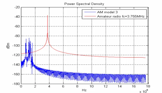
Figure 2.2-3 Amateur radio vs AM model 3 PSD
In Figure 2.2-3, the PSD of amateur radio is lager than AM broadcast radio. Therefore, the main source of RFI is considered to be the amateur radio transmitters. In this thesis, we will focus on dealing with amateur radio.
Figure 2.2-4 The PSD level of RFI vs Received signal
In the Figure 2.2-4 we can observe that RFI significantly degrades VDSL system performance, since RFI which is not periodic in the sub-carriers spacing gets spread to many sub-carriers. This is because the segmentation of the received data and removal of cyclic prefix is equivalent to multiplying the received signal (including RFI noise) by a rectangular window. Multiplication in time is equivalent to convolution in the frequency-domain with a sinc-like function. Since the sidelobes of the sinc are relatively high and decay rather slowly, RFI can effect a large number of sub-channels [11].
In order to satisfy the RFI egress requirements, DMT tones within HAM-band 1~5 are not modulated as shown in Figure 2.2-4. As a result, these unused tones can be used to measure the RFI, and RFI models can be estimated with the help of the measurements.
Chapter 3
Cancellation Of RFI
Since the power of RFI signal may be high. In order to prevent RFI signal clipping in ADC, a front-end analog cancellation which can suppress the RFI power level is needed. DMT-tones in the HAM-bands must be unused in order to avoid RFI egress. So we can use unused tones in the HAM-bands to estimate the RFI signal model. The block diagram of RFI canceller shows as Figure 3-1.
Figure 3-1. Block diagram of RFI canceller
As shown in Figure 3-1, the RFI cancellation process has to be conducted symbol by symbol. The derivation of the RFI signal model from one DMT symbol period is the beginning of our RFI cancellation algorithm. The simplest model is zero-order with a constant RFI envelope in one VDSL symbol period [9]. But in ETSI VDSL systems, the symbol periods are several times longer than that of Zipper VDSL. The RFI envelop in one DMT symbol may not be constant. By the parameters listed below, the relationship between RFI bandwidth and VDSL sub-carrier spacing is explained.
1. RFI bandwidth < VDSL sub-carrier spacing
Zipper-based VDSL’s sampling rate is fixed at 22.08MHz.
2 2 .0 8 1 2 3 .1 8 Z i p p e r V D S L s u b c a r r i e r s p a c i n g : B W = 1 1 .0 4 M H z = 4 3 .1 2 5 s u b c a r r i e r n u m = 2 5 6 1 s y m b o l p e r i o d : R F I b a n d w i d t h = 4 K H z 2 5 0 4 K H z 1 s f M H z s f K H z f s µ µ = = ∆ = ∆ =
If the RFI bandwidth is smaller than the inter-tone spacing of the DMT system, than the base-band function m(t) will not change much with the duration of one DMT frame [8]. Therefore, the RFI envelope is constant.
2. RFI bandwidth ≅ VDSL sub-carrier spacing
ETSI VDSL’s sub-carriers spacing is fixed at 4.3125KHz.
3 5 .3 2 8 1 2 3 1 .8 E T S I V D S L s u b c a rrie r s p a c in g : B W = 1 7 .6 6 M H z = 4 .3 1 2 5 s u b c a rrie r n u m = 4 0 9 6 1 s y m b o l p e rio d : 2 5 0 4 K H z R F I b a n d w id th = 4 K H z 1 s f M H z s f K H z f s µ µ = = ∆ = ∆ =
In this case 1 symbol period (231.8µs) ≈ RFI period (250µs), In ETSI VDSL
systems the RFI envelop in one DMT symbol may not be constant. The simulation of RFI signal in one DMT symbol is shown in Figure 3-2. Therefore, the use of zero-order model in digital RFI cancellation is not fully justified. A
more accurate first-order model is instead adopted by names [11]. In Section 3.2, 3.3, 3.4 we will introduce the previous works in digital RFI cancellation. And our RFI cancellation algorithm is discussed in Section 3.5 and 3.6. In Section 3.7, the reduction of computation cost of our RFI cancellation algorithm will be presented. 0 1000 2000 3000 4000 5000 6000 7000 8000 9000 -0.04 -0.03 -0.02 -0.01 0 0.01 0.02 0.03 0.04
Sampling point (Sampling rate=1/35.328MHz)
Vol
tage
RFI in one DMT symbol
0 1000 2000 3000 4000 5000 6000 7000 8000 9000 -0.025 -0.02 -0.015 -0.01 -0.005 0 0.005 0.01 0.015 0.02 0.025 Vol tage
Sampling point (Sampling rate =1/35.328MHz) RFI in one DMT symbol
0 1000 2000 3000 4000 5000 6000 7000 8000 9000 -0.03 -0.02 -0.01 0 0.01 0.02 0.03
Sampling point (Sampling rate = 1/35.328MHz)
Vol
tage
RFI in one DMT symbol
0 1000 2000 3000 4000 5000 6000 7000 8000 9000 -0.025 -0.02 -0.015 -0.01 -0.005 0 0.005 0.01 0.015 0.02 0.025
Sampling point (Sampling rate = 1/35.328MHz)
Vol
tage
RFI in one DMT symbol
3860 3880 3900 3920 3940 3960 3980 4000 4020 4040 4060 -0.02 -0.015 -0.01 -0.005 0 0.005 0.01 0.015 0.02
Sampling point (Sampling rate = 1/35.328MHz)
Vol tage partial magnification 3850 3900 3950 4000 4050 4100 -6 -4 -2 0 2 4 6 8 x 10⁻³
Sampling point (Sampling rate = 1/35.328MHz)
Vol
tage
partial magnification
3.1 Requirements of RFI Suppression
In order to guarantee reliable VDSL system transmission, at least 20dB
signal to noise ratio (SNR) is needed. Suppose RFI signal band limited to 4KHz bandwidth, the peak value of RFI power spectra density (PSD) is -40dBm/Hz, which is higher than the -60dBm/Hz VDSL PSD mask. Therefore, the RFI canceller should reduce the RFI PSD by 40dB in modulated DMT-tones [6]. But the peak of RFI PSD have no effect on the DSL performance since these tones in the HAM-band is not used. Those tones further away the RFI-peak which the RFI spectral leakage contaminates need RFI suppression since they are used for data transmission. For at least 20dB SNR in modulated DMT-tones, the required level of RFI cancellation shows in Figure 3.1-1. But the sub-carriers with high SNRs can be assigned with more data bits, the desired RFI cancellation level is as much as possible.
The required level of RFI cancellation
20dB 20dB
3.2 Jeong and Yoo’s Approach for Parameter Estimation [9]
The amateur radio S n
[ ]
is transmitted with SSB modulation.[ ]
[ ]
cos(2 ) ˆ[ ]
sin(2 ). (3.2-1)c c
S n = f n π f nT − f n π f nT
where f n
[ ]
is a band-limited signal with a bandwidth of 4KHz, ˆf n[ ]
is a Hilbert pair of f n[ ]
, and is the sampling period of ADC. After N-point Fast Fourier Transform (FFT), this RFI signal is represented asT
[ ]
[ ]
[ ]
[ ]
[ ]
[ ]
[ ]
2 1 0 2 2 1 0 2 2 1 ( ) ( ) 0 [ ] 1 = 2 = . (3 .2 -2 )N j k n N n N j n r j n r j2 n N N n N j n r k j n r k N N n k R k s e f j e f j e e z e z e n n f n n f n n n π π π π π − − = − − − = − − − + ∗ = = + + − + ⎧⎡ ⎤ ⎡ ⎤ ⎫ ⎨⎣ ⎦ ⎣ ⎦ ⎬ ⎩ ⎭ ⎡ ⎤ ⎢ ⎥ ⎣ ⎦
∑
∑
∑
N π Where r f N Tc , fc n T nr, 0 r N/ 2 N = i i i i = ≤ ≤ , and[ ]
1[ ]
[ ]
2 z n = ⎡⎣f n + j f n ⎤⎦ Here,[ ]
f n varies very slowly within
[
0, (N-1)T]
considering the sampling rate, so[ ]
z n can be approximated to a constant within the interval
[
0, (N-1)T]
.Let
[ ]
[ ]
2 ( ) 2 ( ) * 2 2 ( ) ( ) 1 1 . ( 3 .2 -3 ) 1 1 j k r j k r j k r j k r N N e e z n z n R k z z e e π π π π − − − + − − − + − − = ∀ = + − −Let , means the tone index of RFI. means the integer part and means the decimal part.
r= + ∆L
r
L
∆
[ ]
2 ( ) * 2 ( ) 2 2 2 ( ) 2 2 2 ( * * 1 1 ( ) ( = . ( 3 . 2 - 4 ) j L k j L k k L k L j j j j j j N N N N N N k L k L e e R k z z e e e e e e b b a W a W π π π π π π π π − ∆ + − − ∆ + + ∆ − ∆ − − − ∆ ∆ − + − + − − = + − − + − − ) )Where 2 2 2 2 (1 ) j k N k j N j j N W e a e b z e e π π π π − − ∆ − ∆ − ∆ ⎧ = ⎪ ⎪⎪ = ⎨ ⎪ ⎪ = − ⎪⎩
At k=L and L+1, the right hand term of (3.2-4) is negligible, so that
[ ]
[
]
0 1 1 (3.2-5) b b R L R L a W a W ≈ + ≈ − − Then, 0 1 0 [ ] [ 1] ( ) [ ] (3.2-6) [ ] [ 1] W R L W R L a b a W R R L R L − + = = − − + LTherefore, we can estimate the RFI signals by substituting and from (3.2-6) into (3.2-4).
a b
3.3 A Digital RFI canceller by Wise and Bingham [10]
RFI in one DMT symbol [10]
The RF interference is modeled in the time domain as a sinusoid 804 multiplied by a linearly-varying envelope 806. Equation (3.3-1) which follows provides the time domain model.
[
]
( ) ( )(1 ) cos 2 o . (3.3-1)
RFI t =rect t +at π f t+φ
Where rect t( ) is a rectangular window, fo is a carrier frequency of the radio interference, a is a small positive constant, and φ is a phase offset. This time domain model is equivalent to fitting a first-order polynomial to the modulation
envelope of the RF interference within the time duration of a DMT symbol. Equation (3.3-2) which follows details the conversion to the frequency domain.
{
}
( )
2sin cos sin
( )(1 ) . (3.3-2) 2 f a f F rect t at j f f f π π π π π π ⎧ ⎡ ⎤⎫ ⎪ ⎪ + =⎨ + ⎢ − ⎥⎬ ⎢ ⎥ ⎪ ⎣ ⎦⎪ ⎩ ⎭
The Fourier Transform of the cosine function of Equation (3.3-1) is a Dirac function at +f and –f. The negative frequency delta function is ignored because its contribution at the positive frequencies is minimal.
Let fo =(n+ ∆δ) f , where n is a frequency tone number, and δ (0<δ <1).
( ) (3.3-3) ( ) o f m n f f f m δ f = + ∆ − = − ∆
The resulting frequency domain model is as defined in Equation (3.3-4) which follows. 2 . (3.3-4) ( ) n m A B RFI m δ m δ + ⎡ ⎤ =⎢ + ⎥ − − ⎣ ⎦
Where RFIn m+ is the RF interference to frequency tone due to RF
interference
m
(n+δ) , where A and B are complex numbers that must be determined for each symbol. Further, if non-rectangular windowing is also used with the frequency domain model, the effect of the windowing can be approximated by Equation (3.3-5).
{
}
{
}
{
}
2 ( ) | ( ) | ( ) | sin ( ) . (3.3-5) ( ) f m f m m f m n m m F win t F win t W F rect t c m A B RFI W m δ m δ = = = + = = ⎡ ⎤ =⎢ + ⎥ − − ⎣ ⎦Instead of using three frequency tones to precisely determine A and Band δ , the offset amount δ can be approximated by the following Equation (3.3-6).
1 1 0 ( 1)/W . (3.3-6) ( 1)/W ( )/W RFI n RFI n RFI n δ = + + +
Then, using Equation (3.3-5) for tones n and n+1, two Equations (3.3-7, 3.3-8) can be written. 2 0 1 2 0 . (3.3-7) . (3.3-8) 1 (1 ) n n X A B W X A B W δ δ δ δ + = − + = + − −
The complex parameters A and B are determined by the following Equation (3.3-10). 2 0 2 1 1 1 1 . (3.3-10) 1 (1 ) n n X W A B X W δ δ δ δ + ⎡ ⎤ ⎢ ⎥ − ⎡ ⎤ ⎡ ⎤ ⎢ ⎥ = ⎢ ⎥ ⎢ − ⎥⎢ ⎥ ⎣ ⎦ ⎣ ⎦ − ⎢ ⎥ ⎣ ⎦
Furthermore, high order models could be likewise used to provide an even more
accurate model for the RF interference:
1 1 , (3.3-11) ( ) MO k n m k k A RFI m δ + + = ⎡ ⎤ = ⎢ − ⎥ ⎣
∑
⎦where MO is a model order for the frequency domain model, and are complex numbers that are determined at each symbol for each interferer.
k
A
3.4 A Iterative RFI canceller by Huang [7]
In VDSL system the number of sub-carriers is large (N=2N’=4096 or
N=2N’=8192), so we can assume 2 1 j N a e π − ∆ = ≈ . 1. Equation (3.2-4) becomes: [ ] . (3.4-1) 1 k L 1 k L b b R k W W ∗ − + = + − −
2. Record RFI components in the HAM-band for iterative cancellation:
[ ] ham band
R − k : RFI signals in the HAM-band.
3. Choose an unused tone in the HAM-band which RFI appears (except L, which will cause dividing by zero) to derive b1.
1 2 1 1 1 [ 1] . (3.4-2) 1 1 L b b R L W W ∗ + + = + − −
Since , are complex, we can use (3.4-3) to find the real and image part. 1 b R L[ + ]1
{ }
{ }
{ }
{ }
{ }
{ }
{ }
{ }
{ }
{ }
{
}
{
}
1 1 2 1 1 2 1 1 2 2 1 1 2 1 1 2 1 1 2 1 2 Re 1 Re [ 1] Im 1 Im [ 1] 1 Re 1 Re Im Im Im Im 1 Re 1 Re(3.4-3)
.
L L L L b R b R W W W W C C C C W W W W C C C C − + + + + + + − − − + = − − + −
⎡
+
⎤
⎢
⎥
⎡
⎤
⎢
⎥
⎡
⎤
⎢
⎥
⎢
⎥
⎣
⎦
⎢
⎥
⎣
⎦
⎢
⎥
⎣
⎦
L L And{ }
{ }
{
}
{
}
2 2 1 1 1 2 2 2 2 1 2 (1 Re ) (Im ) (1 Re L ) (Im L ) . C W W C W + W + = − + = − + 14. By substituting into (3.4-1), the estimated RFI components in the HAM-band can be subtracted form
1 b [ ] ham band R − k . 1 [ ] [ ] R [ ]
residual ham band estimated b
R k =R − k − − k
5. Choose another tone in Rresidual[ ]k to derive b2, as in step 3.
Take Rresidual[L−1] for example:
{ }
{ }
{ }
{ }
{ }
{ }
{ }
{ }
{ }
{ }
{
}
{
}
1 1 2 1 1 2 1 1 2 2 1 1 2 1 1 2 1 1 2 1 2 Re [ 1] Re 2 Im [ 1] Im 2 1 Re 1 Re Im Im Im Im 1 Re 1 Re.
L L L L residual residual R L b R L b W W W W C C C C W W W W C C C C − − − − − − − − − − − − − − + = − − +
⎡
+
⎤
⎢
⎥ ⎡
⎤
⎡
⎤ ⎢
⎥ ⎢
⎥
⎢
⎥
⎣
⎦
⎢
+
⎥
⎣
⎦
⎢
⎥
⎣
⎦
6. By substituting b2 into (3.4-1), then
2
[ ] [ ] R [ ]
residual ham band estimated b
R k =R − k − − k
achieved. ( R [ ]k [ ] residual ham band small enough R − k → )
8. Finally, by substituting (b1+b2+…+bN) = b into (3.4-1), the estimated RFI components at each tone can be subtracted form received RFI to achieve RFI suppression.
3.5 An RFI Signal Model (Model 1)
The amateur radioSrfi( )t is transmitted with SSB modulation.
( ) ( ) cos(2 ) ( ) sin(2 ) (3.5-1) rfi c c S t =m t π f t −m t π f t [ ] [ ] cos(2 ) [ ]sin(2 ) (3.5-2) rfi c c S n =m n πf nT −m n πf nT
Where m t( )is speech signal band limited to 4KHz bandwidth, m t( ) is the
Hilbert transform of , and is the sampling period of ADC. The simplest, zero-order model of the envelope is a constant in one DMT symbol period [9]. With SDMT (Synchronize DMT) parameters (with a 1:10 ratio of the 25
( )
m t
T
s
µ symbol period to the shortest cycle of the 4KHz RFI signal), this model is
quite good, and 40~50 dB of RFI suppression can be achieved [2]. But one symbol period in ETSI VDSL system is several times longer than SDMT, thus the assumption of constant envelope is unrealistic. In our approach, the basic idea is to use a slowly-sinusoid wave as the model of the envelope of RFI in one DMT symbol. symbol 1 2 ( ) ( )( cos(2 )) cos(2 ) (3.5-3) 1 for 0<t<T ( ) 0 otherwise
rfi e i S t rect t c d f t f t rect t π φ π φ = + + + =
⎧
⎨
⎩
of RFI in one DMT symbol as shown in Fig 3-2.
e
f is the frequency of speech signal in one DMT symbol.
i
f is not the HAM carrier frequency, which will typically be constant over
many symbols. But rather, fi is a pseudo center frequency which displaced 1
to 2 kHz from the carrier frequency because of the SSB modulation. Therefore,
i
f will change from symbol to symbol [2].
T
is the sampling period of ADC. The discrete signal reads as:1 2
( cos( 2 )) cos( 2 ). (3.5-4)
[ ]
rfi e i
S
n
=
c + d π fnT
+φ π fnT
+φAfter N (=2N’)-point Fast Fourier Transform (FFT), the RFI signal is
represented as: 2 1 0 [ ] [ ]
0,1, 2...
1
N j kn N rfi n R k S n ek
N
π − − = =∑
=
−
The operation process is described in Appendix A. In a more concise form,
1 1 2 2 3 3 1 1 2 ( ') 2 ( ') 3 ( ') 3 ( ') [ ] (3.5-5) k L k L k L L k L L k L L k L L b b b b b b R k a W a W a W a W a W a W ∗ ∗ ∗ ∗ ∗ ∗ − + − + + + − − + − = + + + + + − − − − − − where 2 2 2 ( ) 1 1 2 2 ( ') 2 ( ') 2 ( ( ')) 2 2 2 ( ') ( ') 2 ( ') 2 ( ') 2 ( 3 3 2 ( ') ( ') 2 1 2 2 1 ( ) ( ) 1 2 1 4 1 4 j j j k L N N k L j N j j j k L L N N k L L j N j j j k N N k L L j N j j j c e a e b e W e e d e a e b e W e e d e a e b e W e e π π π π π π π π π π π π φ φ φ φ φ ∆ ∆ − − − − ∆ ∆ + ∆ ∆ + ∆ − − − + − + ∆ + ∆ ∆ − ∆ ∆ − ∆ − − − − − ∆ − ∆ + − − = = = − = = = − = = =
⋅
⋅
⋅
( ')) . L−L⎧
⎪
⎪
⎪
⎪⎪
⎨
⎪
⎪
⎪
⎪
⎪⎩
In VDSL system the number of sub-carriers is large (N=2N’=4096 or N=2N’=8192), so we can assume that , and can be approximated by 1. But this assumption will influence the accurate of RFI signal model. The details are described in the section 3.5.2 (Measurement tones selection).
1
a a2 a3
Furthermore, with the assumption that speech signal band limited to 4KHz we can set L'=0 . Finally, The RFI signal model becomes as:
1 2 3 1 2 3 ( ) ( ) [ ] 1 1 0 . .. .. - 1 1 1 k L k L k L k L b b b b b b R k W W b b k N W W ∗ ∗ ∗ − + ∗ − + + + + + = + − − = + = − − (3.5-6)
Equation (3.5-6) is the same as equations found in [7]. But here a different strategy is used to cancel the RFI.
3.5.1 RFI detection and parameter estimation
Since the information about the RFI is unknown, we need to do RFI detection in advance. To detect the RF interference we can use a method that finds the maximum absolute value among the FFT tones inside the HAM bands and compares it with a threshold. The value of the threshold will vary with system design but is normally set 20dB above the noise floor. When the maximum absolute data vector ( R k[ ']) is greater than the threshold, then the RFI
cancellation process is started.
One way to find L is described in [10]. The main idea of this method is
equation (3.5-7) list below. By searching unused tones (the max value ( )
and the second max value ( ), we could find
[ ']
R k
[ '']
_ ' _ ''
[ ']
[ '']
[ ']
[ '']
(3.5-7)
[
1]
[ ]
[
1]
index k index k LR k
R k
R k
R k
R L
R L
R L
+ = + ∆ + ∆ =⎧
⎪
⎪
⎨
+
⎪
⎪
+
+
⎩
i i [ '] R k [ ''] R k [ '] R k [ ''] R k∆
∆
Figure 3.5-1 Illustration for the cases
Based on (3.5-6), if we consider 1 unused tone in the HAM-band we can use it as a known number (by measuring a tone in the HAM-band) to calculate . We finally obtain the expression of the RFI estimation on all DMT tones. Since and are complex, we can use (3.5-8) to find the real and image part, according to [7].
1 [ ] R k b b R k[ ]1
{
}
{
}
{ }
{ }
{ }
1{ }
1{ }
{ }
1{ }
{ }
1 1 Re Im Re Im Re [ ] Im [ ] (1 Re ) (Im ) (1 Re ) (Im ) k L k L k L k L b j b b j b R k j R k W − j W − W + j W + − + = + − − − −{ }
{ }
1+{ }
{ }
{ } { }
{ } { }
{ }
{ }
{
}
{
}
1 1 1 1 1 1 1 1 1 1 1 1 2 2 1 1 2 1 2 Re [ ] Re Im [ ] Im 1 Re 1 Re Im Im Im Im 1 Re 1 Rek L k L k L k L k L k L k L k L R k b R k b W W W W C C C C W W W W C C C C − − + + − − + − + − − + − = − − + −
⎡
⎤
⎢
⎥
⎡
⎤
⎡
⎤ ⎢
⎥
⎢
⎥
⎢
⎥ ⎢
⎥
⎣
⎦
⎣
⎦
⎢
⎥
⎢
⎥
⎣
⎦
8)
And
{
}
{
}
{
11}
{
11}
2 2 1 2 2 2 (1 Re ) (Im ) (1 Re ) (Im ) . k L k L k L k L C W W C W W − − + + = − + = − +Based on (3.5-6), the second term represents the negative-frequency term, which can be ignored if the RFI center frequency is far from DC or Nyquist frequency. Therefore, its contribution at the positive frequencies is minimal and we can further simplify (3.5-8) into (3.5-9).
1
1
[ ] (1 k L )
b = R k −W − (3.5-9)
Which together with (3.5-6) complete the RFI model.
3.5.2 Measurement tones selection
How do we choose the placement of measurement tones? In the simulation, the placement of measurement tones has a great impact on RFI estimation. When the measurement tones are very close to the RFI-peak, the estimation error of RFI model will increase, but the measurement SNR (RFI /noise) is good. When the measurement tones are placed further away from the RFI-peak, the estimation error of RFI model is less, but SNR is lower. This kind of situation is also mentioned in [8].We use simulation and RFI model analysis to explain the issue of measurement tones selection.
A simulated typical RFI signal is used as an example:
symbol 1 2 ( ) ( )( cos(2 )) cos(2 ) = ( )(0.03+0.007 cos (2 4KHz t+1.8436 ))cos(2 3.755MHz t+1.4764 )) 1 for 0<t<T ( ) 0 otherwise
rfi e i S t rect t c d f t f t rect t rect t π φ π φ π π π π = + + + ⋅ ⋅ ⋅ ⋅ ⋅ =
⎧
⎨
⎩
Figure 3.5-2 A given RFI signal in one DMT symbol period
With these given parameter ( c , d , fe , fi ,φ1 ,φ ), we can calculate the 2
theoretical value of RFI. The simulation diagram shows in Figure 3.5-3 and 3.5-4. In Figure 3.5-4 (b), the simplify RFI model (3.5-6) is not accurate at tones close to the RFI-peak. Hence, If we use a measurement tone close to the RFI-peak as a known number to calculate , the estimation error of will increase. For reducing the estimation error of , we must use a measurement tone further away the RFI-peak to calculate .
1 [ ] R k b b b b 0 500 1000 1500 2000 2500 3000 3500 4000 4500 -400 -350 -300 -250 -200 -150 -100 -50 0 tone unmber dB m /Hz
power spectral density
RFI signal residual RFI 845 850 855 860 865 870 875 880 885 890 895 0 10 20 30 40 50 60 70 80 90 100 tone number ab s( R F I)
RFI signal after FFT RFI signal
RFI signal estimation
(a) (b)
0 500 1000 1500 2000 2500 3000 3500 4000 4500 -200 -180 -160 -140 -120 -100 -80 -60 -40 -20 tone number dB m /H z
power spectral density
RFI signal residual RFI 860 865 870 875 880 885 890 0 20 40 60 80 100 tone number ab s( R F I)
RFI signal after FFT
RFI signal RFI estimation
(a) (b)
Figure 3.5-4 Simplify RFI model (3.5-6) cancellation
Furthermore, we use RFI model analysis to explain the issue of measurement tones selection. 1 1 2 2 3 3 1 1 2 ( ') 2 ( ') 3 ( ') 3 ( ') [ ] . (3.4-5) k L k L k L L k L L k L L k L L b b b b b b R k a W a W a W a W a W a W ∗ ∗ ∗ ∗ ∗ ∗ − + − + + + − − + − = + + + + + − − − − − − 1 1 1 2 3 * simplify * -2 2 - - (k -L) [ ] [ ] Let '= 0, 0... -1 0... -1 - - 1 1 Assume 1- , = =1-k L k L k L k L j j N N k L R k R k L a a a a b b b b k N k N a W a W W W a e i W e i π π
ε
δ
∗ + − ∆ − = = ≅ ≅ ≅ + = ⎯⎯⎯→ + = − − = = + iWe can ignore negative-frequency term, and find out b.
Theoretical value b=R k[ ] ( -1 ⋅ a Wk L1- )= [ ] ((1-R k1 ⋅
ε
i) (1-−δ
i)) =R k[ ] (1 ⋅δ
−ε
) Estimation value b=R k[ ] (1-1 ⋅ Wk L1- )= [ ] (1-R k1 ⋅ Wk L1- )= [ ] (1-(1- ) )R k1 ⋅δ
i =R k[ ]1 ⋅δ
i Estimation error b = Estimation value - Theoretical valueEstimation error b = [R k1] ⋅
ε
iIn the Figure 3.5-3 (b), we can observe the magnitude of the measurement tone decreases if it is further away the RFI-peak. Therefore, the estimation error decreases.
3.6 First order model (Model 2)
If we use first-order model, the RFI model shows as bellow.
s y m b o l ( ) ( ) c o s ( 2 ) ( 3 . 6 - 1 ) 1 f o r 0 < t < T ( ) 0 o t h e r w i s e . ( ) r f i i S r e c t t c d t f r e c t t t = + π t φ = ⎧⎨ ⎩ + 2 ( ) cos(2 ) ( ) cos( ). (3.6-2) rfi i S n c d n fnT c d n nr N π π +φ φ ⎡ ⎤ ⎣ ⎦= + ⋅ = + ⋅ +
After N (=2N’)-point Fast Fourier Transform (FFT), the RFI signal is
represented as: 2 1 0 [ ] [ ]
0,1, 2...
1.
N j kn N rfi n R k S n ek
N
π − − = =∑
=
−
The operation process is described in Appendix B. In a more concise form,
1 1 2 2 3 3 2 2 1 1 1 1 1 1 1 1 [ ] [ ( )] [ ( )] (3.6-3) k L k L k L k L k L k L k L k L b b b b W b W b R k a W a W a W a W a a W a a W ∗ ∗ ∗ − + ∗ ∗ ∗ ∗ − + − + − + ⋅ ⋅ = + + + + + − − − − − − Where 2 2 1 2 2 2 2 1 2 3 (1 ) 2 2 . (1 ) 2 j j N j j j N j j N j j c b e e e d b N e e e a e d b e e π π φ π π φ π π φ − ∆ ∆ − ∆ ∆ − ∆ ∆ ⎧ ⎪ ⎪ ⎪ = − ⋅ ⋅ ⋅ ⎪⎪ ⎨ ⎪ = − ⋅ ⋅ ⋅ ⋅ ⎪ ⎪ ⎪ ⎪⎩ = = − ⋅ ⋅
In VDSL system the number of sub-carriers is large (N=2N’=4096 or N=2N’=8192), so we can assume thata1is approximated by 1.
Finally, The RFI signal model becomes as:
3 3 2 2 [ ] (3.6-4) 1 1 (1 ) (1 ) k L k L k L k L k L k L W b W b b b R k W W W W ∗ ∗ − + − + − + ⋅ ⋅ = + + + − − − −
Where 1 2 2 1 2 1 2 2 3 1 (1 ) 2 2 (1 ) . 2 j j j j j a c d b e e b N e e b b b d b e e j π φ π φ π φ ∆ ∆ ∆ ≅ ⎧ ⎪ ⎪ ≅ − ⋅ ⋅ ≅ − ⋅ ⋅ ⋅ ⎪ ⎨ = + ⎪ ⎪ ≅ − ⋅ ⋅ ⎪ ⎩
Based on (3.6-4), 2 unused tones in the HAM-band are used as the known numbers and (by measuring 2 tones in the HAM-band) to
calculate and . Since , , and are complex, we can use (3.6-5) to find the real and image part.
1 [ ] R k R k[ 2] b b3 b b3 R k[ ]1 R k[ 2] { } { } { } { } { } { } { } { } 1 1 3 2 3 2 1 11 12 13 14 21 22 23 24 31 32 33 34 41 42 43 44 Re Re [ ] Im Im [ ] Re Re [ ] Im Im [ ] (3.6-5) b R b R b R b R M M M M M M M M M M M M M M M M − ⎡ ⎤ ⎡ ⎤ ⎡ ⎤ ⎢ ⎥ ⎢ ⎥ ⎢ ⎥ ⎢ ⎥ ⎢ ⎥ = ⎢ ⎥ ⎢ ⎥ ⎢ ⎥ ⎢ ⎥ ⎢ ⎥ ⎢ ⎥ ⎢⎣ ⎥⎦ ⎣ ⎦ ⎢⎣ ⎥⎦ k k k k k k k k 1 1
The detail (M11, M12……) is described in Appendix C.
In accordance with Section 3.5.1 we can ignore the negative-frequency term. Similarly (3.6-5) is further simplified into (3.6-6).
{ } { } { } { } { } { } { } { } 1 1 3 2 3 2 1 11 12 13 14 21 22 23 24 31 32 33 34 41 42 43 44 Re Re [ ] Im Im [ ] Re Re [ ] Im Im [ ] (3.6-6) b R b R b R b R M M M M M M M M M M M M M M M M − ⎡ ⎤ ⎡ ⎤ ⎡ ⎤ ⎢ ⎥ ⎢ ⎥ ⎢ ⎥ ⎢ ⎥ ⎢ ⎥ = ⎢ ⎥ ⎢ ⎥ ⎢ ⎥ ⎢ ⎥ ⎢ ⎥ ⎢ ⎥ ⎢⎣ ⎥⎦ ⎣ ⎦ ⎢⎣ ⎥⎦ 2 2 2 2 4 4 3 3 3 3 3 (1 ) (1 2 )
1 2 Re{ } Re{ } ( 2 Im{ } Im{ })
Re{ } Re{ } Im{ } Im{ } (Im{ } Re{ } Im{ } Re{ })
where k L k L k L k L k L k L k L k L k L k L k L k L W W W W W j W W X jY W b W b W b j W b b W X jY − − − − − − − − − − − − − = − ⋅ + = − + + − + = + ⋅ = ⋅ − ⋅ + ⋅ + ⋅ = +
{
}
2 1( ) 2 2 3( ) 4 4 (1 Re ) k k k C W C X Y − = − = + L{ }
{ }
{ }
{ }
{ }
{ }
{ }
{ }
{ }
{ }
{ }
1 1 1 1 1 1 1 1 1 1 1 11 1( 1) 4 4 21 22 23 24 1( 1) 1( 1) 3( 1) 4 4 4 12 13 14 1( 1) 3( 1) 3( 1) 1 Re Im 1 Re Im Re Re Im Re Im Im Re K L k K L K L K L K L K L k k k K L K L K L K L K L k k k W M C W W W X W Y W M M M M C C C W W X W Y W X W M M M C C C − − − − − − − − − − − − = − ⋅ − ⋅ ⋅ = = = = ⋅ + ⋅ − ⋅ + ⋅ =− = ={ }
4 Y{ }
{ }
{ }
{ }
{ }
{ }
{ }
{ }
{
}
{ }
1 2 2 2 2 2 2 2 2 2 4 4 3( 1) 4 4 4 4 31 32 33 34 1( 2) 1( 2) 3( 2) 3( 2) 2 4 4 41 42 43 1( 2) 1( 2) 3( Im 1 Re Im Re Im Im Re Im 1 Re Im Re K L k K L K L K L K L K L K L k k k k K L K L K L K L k k X W Y C W W W X W Y W X W Y M M M M C C C C W W W X W Y M M M C C C − − − − − − − − − − − + ⋅ − ⋅ + ⋅ − ⋅ = =− = = − ⋅ − ⋅ = = = + ⋅{ }
2 4{ }
2 4 44 3( 2) 2) Re Im K L K L k k W X W Y M C − ⋅ + − ⋅ =3.7 Reduce computation cost of RFI cancellation algorithm
For model 1, the computation cost is as follows.
1
1
[ ](1
)
need 1 complex multiplication
[ ]
0...
-1
need 2N complex divisions
1
1
k L k L k Lb
R k
W
b
b
R k
k
N
W
W
− ∗ − +=
−
⇒
=
+
=
⇒
−
−
Computation cost = 2N complex divisions + 1 complex multiplication.
In physical implementation, the division is not desirable. In general, the divisions are mostly replaced by multiplication or looking up table. However, the equation (3.5-6) can be modified into a more computation-friendly form. Start with 2 ( ) (1 ) 1 cos sin 2 2 cos 2(1 co 1 1 1(1 ) (1 ) 1 (1 )(1 ) 2 ( ) 1 [ ] 0 : 1, 1 1 ( , 2 )
Let
then
j j j j j j j j k L k L N k L k L e j e e W e e e e e b b R k k N k L W W k L N θ θ θ π θ θ θ θ θ θ θ π θ − − − − − − − − − − − − ∗ − + − − − − − − − = = − − − − = = = − − − − − + = + = − ≠ − − = − 2 2 21 sin sin (1 cos )
s ) 2 2(1 cos ) 2(1 cos )(1 cos )
sin (1 cos ) sin (1 cos )
0.5 0.5 2(1 cos ) 2 sin 0.5 (1 cos ) 0.5 0.5 sin 2cos 2 0.5 0.5 0.5 sin j j j j j j j θ θ θ θ θ θ θ θ θ θ θ θ θ θ θ θ − − − − − − θ − − − − − − − − − − + = − − − + + = − − − = − + = − ⋅ = − ⋅ = − = − + 2 2 ( ), 1 1 sin 1 2 2 2 cos 2 2cos 2 0.5 0.5 0.5 cot 2 2sin cos 2 2 0.5 0.5 cot And then k L k L N j W j j π θ θ θ θ θ θ θ θ + + + + − − − − + = + = − − − ⋅ = − ⋅ ⋅ = − ⋅
( ) ( ) , [ ] 0.5 0.5 cot 0.5 0.5 cot 0 : 1, (3.7 1) where
Therefore
k L k L N N R k b j b j k N k L π π θ θ θ− ∗ θ+ − = − + = + ⎡ ⎤ ⎡ ⎤ = ⋅⎣ − ⋅ ⎦+ ⋅⎣ − ⋅ ⎦ = − ≠ −Base on equation (3.7-1), we can simplify the computation cost of our RFI cancellation algorithm. In (3.7-1) the trigonometric function be implemented by CORDIC algorithm [13] that is performed by a shift and add operation. As a result, the implementation would be easier.
[ '] R k [ '] threshold R k ≥ [ ] R k
Chapter 4
Multiple RFI Cancellation
In VDSL transmission environment there may be more than one amateur radio users simultaneously. Therefore, multiple RFIs should be considered. Two cases of multiple RFIs are described as follows:
Case1: There is only one RFI source in each HAM-band. In this case the interference between RFI_1 (RFI in HAM-band1) and RFI_2 (RFI in
HAM-band2) can be negligible. Under this assumption we can use the single RFI algorithm (3.5-6) to deal with RFI_1 and RFI_2, respectively.
Case2: There are more than one RFI sources in a HAM-band [7]. Based on the algorithm of RFI estimation (3.5-6), we can extend (3.5-6) form single RFI to multiple RFIs. The two RFI model becomes as:
1 1 2 2 1 1 2 2 1 2 [ ] 1 1 1 1
( 4 -1 )
0 :
1,
,
.
k L k L k L k L b b b b R k W W W Wk
N
k
L
L
∗ ∗ − + − + = + + + − − − −=
−
≠
The conjugate term represents the negative-frequency term, which can be ignored if the RFI center frequency is far from DC or Nyquist frequency. Therefore, its contribution at the positive frequencies is minimal and we can further simplify (4-1) into (4-2).
1 2 1 2 1 2 [ ] 1 k L 1 k L
0 :
1,
,
. (4 -2 )
b b R k W − W −k
N
k
L L
= + − −=
−
≠
Based on (4-2) we need two unused tones (R k[ 1],R k[ 2]) to calculate and . 1 b 2 b 1 1 1 2 2 1 2 2 1 2 1 - -1 2 2 - -[ ] 1 - 1 -[ ] 1 - 1 -
.
k L k L k L k L b b R k W W b b R k W W = + = +⎧
⎪⎪
⎨
⎪
⎪⎩
We can use a inverse of 4×4 matrix (4-3) to find
b
1 andb
2.{ }
{ }
{ }
{ }
{
}
{
}
{
}
{
}
{
1 1}
{
1 1}
1 1 11 12 13 14 1 1 21 22 23 24 1 2 31 32 33 34 2 2 41 42 43 44 2 11 12 13 1(1) 1(1) Re Re [ ] Im Im [ ] (4-3) Re Re [ ] Im Im [ ] 1 Re Im 1 R where K L K L b M M M M R k b M M M M R k b M M M M R k b M M M M R k W W M M M C C − − − ⎡ ⎤ ⎡ ⎤ ⎡ ⎤ ⎢ ⎥ ⎢ ⎥ ⎢ ⎥ ⎢ ⎥=⎢ ⎥ ⎢ ⎥ ⎢ ⎥ ⎢ ⎥ ⎢ ⎥ ⎢ ⎥ ⎢ ⎥ ⎢ ⎥ ⎢ ⎥ ⎢ ⎥ ⎣ ⎦ ⎢ ⎥ ⎣ ⎦ ⎣ ⎦ − − = = − ={
}
{
}
{
}
{
}
{
}
{
}
{
}
{
}
{
}
{
}
1 2 1 2 1 1 1 1 1 2 1 2 2 1 2 1 2 2 2 2 2 14 ' ' 1(1) 1(1) 21 22 23 ' 24 ' 1(1) 1(1) 1 1(1) 31 32 33 ' 34 ' 1(2) 1(2) 1(2) 1(2) 41 e Im Im 1 Re Im 1 Re 1 Re Im 1 Re Im Im K L K L K L K L K L K L K L K L K L K L K W W M C C W W W W M M M M C C C C W W W W M M M M C C C C W M − − − − − − − − − − = − − − = = = = − − = = − = = − ={
}
−{
}
{
}
{
}
1 2 1 2 2 42 43 ' 44 ' 1(2) 1(2) 1(2) 1(2) 1 Re Im 1 Re L WK L WK L WK M M M C C C C − − − − − = = ={
}
2 L2{
}
{
}
{
}
{
}
{
}
{
}
{
}
1 1 1 1 1 2 1 2 2 1 2 1 2 2 2 2 2 2 1(1) ' 2 2 1(1) 2 2 1( 2 ) ' 2 2 1( 2 ) (1 R e ) (Im ) (1 R e ) (Im ) (1 R e ) (Im ) (1 R e ) (Im ) . K L K L K L K L K L K L K L K L C W W C W W C W W C W W − − − − − − − − = − + = − + = − + = − +We finally obtain the expression of 2 RFI signal model estimation (4-4) on the N DMT tones.
1 1 1 1 2 2 2 2 1 ( 1) 1 ( 1) 2 ( 2) 2 ( ) [ ] 0.5 0.5 cot 0.5 0.5 cot + 0.5 0.5 cot 0.5 0.5 cot (4-4) 0 : 1, k L k L k L k L N N N N R k b j b j b j b j k N π π π π θ θ θ θ θ θ θ θ − ∗ + − ∗ + − = − + = + − = − + = + ⎡ ⎤ ⎡ ⎤ = ⋅⎣ − ⋅ ⎦ + ⋅⎣ − ⋅ ⎦ ⎡ ⎤ ⎡ ⎤ ⋅⎣ − ⋅ ⎦ + ⋅⎣ − ⋅ ⎦ = − k ≠ L L1, 2 2
The algorithm of multiple RFI can be used in case1, too. And that the RFI signal model in case1 will be more accurate, but it will increase the modeling difficulty. The computational complexity for multiple-RFI models is shown:
2 RFI inverse of 4×4 matrix
3 RFI inverse of 6×6 matrix
N RFI inverse of 2N×2N matrix
Similarly, we can extend (3.6-4) from single RFI to multiple RFIs. However, the computation is too costly. The straight forward extension is omitted here.
![Figure 1.2 VDSL Deployment Configuration [14]](https://thumb-ap.123doks.com/thumbv2/9libinfo/8504370.185428/13.892.133.806.120.443/figure-vdsl-deployment-configuration.webp)

![Figure 1.3-3 VDSL Deployment Configuration alien crosstalk [14]](https://thumb-ap.123doks.com/thumbv2/9libinfo/8504370.185428/15.892.133.806.120.435/figure-vdsl-deployment-configuration-alien-crosstalk.webp)
![Figure 1.3-5 An example of RFI egress [12]](https://thumb-ap.123doks.com/thumbv2/9libinfo/8504370.185428/16.892.217.768.108.368/figure-an-example-of-rfi-egress.webp)
![Table 2.1-1 signal strengths for AM radio noise into VDSL [3]](https://thumb-ap.123doks.com/thumbv2/9libinfo/8504370.185428/19.892.161.770.474.982/table-signal-strengths-radio-noise-vdsl.webp)
![Table 2.2 Amateur Radio Bands defined by ANSI [3]](https://thumb-ap.123doks.com/thumbv2/9libinfo/8504370.185428/22.892.188.752.100.484/table-amateur-radio-bands-defined-ansi.webp)