國 立 交 通 大 學
電子工程學系 電子研究所碩士班
碩 士 論 文
H.264/MPEG-4 AVC 移動估測的快速演算法與架構設計
Fast Algorithms and Architecture Designs for H.264/MPEG-4
AVC Motion Estimation
研究生: 王裕仁
指導教授: 張添烜
H.264/MPEG-4 AVC 移動估測的快速演算法與架構設計
Fast Algorithms and Architecture Designs for H.264/MPEG-4 AVC
Motion Estimation
研 究 生: 王裕仁 Student: Yu-Jen Wang 指導教授: 張添烜 博士 Advisor: Tian-Sheuan Chang
國 立 交 通 大 學 電子工程學系 電子研究所碩士班
碩 士 論 文
A Thesis
Submitted to Department of Electronics Engineering & Institute of Electronics College of Electrical Engineering and Computer Science
National Chiao Tung University in Partial Fulfillment of Requirements
for the Degree of Master of Science
In
Electrical Engineering June 2006
Hsinchu, Taiwan, Republic of China
誌 謝
首先,要感謝我的指導教授—張添烜博士,這兩年來給我的支持和鼓勵,讓 我在研究上能自由發揮,每當遇到問題和疑問時總能適時的給予最適當的建議, 當意見相左時也往往能夠給予最大的尊重,永遠以鼓勵的態度支持我的想法。張 老師的溫文儒雅作風也讓我莽莽撞撞的個性有潛移默化的改變,感激之情,非數 十字可以言表。 也要謝謝我的口試委員們,交大電子李鎮宜系主任和清華大學陳永昌教授, 感謝你們百忙中抽空來指導我,因為你們寶貴的意見讓我的論文更加完備。 接著要感謝 VSP 實驗室的好伙伴們。謝謝引我入門的鄭朝鐘學長,給予不少 建議的張彥中學長、林佑坤學長,你們傳給我的經驗,將讓我受用不盡。感謝古 君偉同學,參加 IC 競賽的過程,一起加油打氣,培養出短時間內迅速確實完成 設計的能力。感謝蔡旻奇、吳錦木同學,在面對冷澀堅硬的研究之餘,一起興致 高昂的出遊踏青,醞釀出下次更具爆發力的創意。感謝余國亘同學、郭子筠學弟, 在團體競爭的刺激下,領悟出團體中個人角色如何定位,爲踏出社會做先一步的 準備。感謝史彥芪學長、林嘉俊、吳秈璟、廖英澤、李得瑋學弟們,有你們的陪 伴,我的碩士班生涯充滿了歡笑。所有的一切,都是我在交大寶貴的回憶。 最後要感謝默默支持我的家人們,我的爸媽、哥哥、姊姊,你們的溫暖是我 努力最大的支柱。 在此,把本論文獻給所有愛我與所有我愛的人。I
H.264/MPEG-4 AVC 移動估測的快速演算法與架構設計
研究生: 王裕仁 指導教授: 張添烜 博士 國立交通大學電子研究所碩士班 摘 要 隨著高解析數位電視時代的來臨,為了兼顧大且精緻的畫面,高壓縮率規格 (H.264)是我們現行的解決方案。它不僅可有效節省儲存媒體所需的空間,同時 也可在現行的通訊環境下允許傳輸更高解析的畫面。伴隨著種種好處而來的就是 極之龐大的運算量,而大量的快速演算法也因此應運而生。如何兼顧畫質和運算 速度成了當前最重要的課題,而這也是本篇論文的主旨。 根據已出版的文獻,位移估測是整個壓縮過程中最為費時的。更進一步去了 解這個部份,我們可以把他大致上分為整數位移估測和分數位移估測。在原始演 算法的條件下,由於搜尋範圍較大整數位移估測佔去了絕大部分的時間。因此我 們非常直覺的認為,若能大幅減少搜尋範圍又能使畫質維持差不多水準將可以有 效節省壓縮時程,我們提出的快速演算法能夠針對不同解析畫面達到 88% (352 x 288)和 75%(720 x 480)的節省。分數位移估測在原始演算法的架構下,由於搜 尋點數遠少於整數位移估測所以在整個壓縮的過程中並沒有決定性的影響。但隨 著整數位移估測快速演算法的發展,分數位移估測搜尋點數所佔的比例慢慢升 高,分數位移估測快速演算法也愈來愈有存在的必要性。在單一樣式錯誤表面的 假設下,我們利用特定點的錯誤數值去預測整個搜尋視窗的錯誤表面。除此之 外,我們也引進了提前終止的技術。此分數快速位移估測部分可以減少超過 50% 的運算量。在整數和分數位移估測同時使用快速演算法的情形下,以 1280 x 720 為測試解析度,我們可以加速總壓縮時間達 20 倍之鉅。另外一種常見的解決方 式是利用硬體平行化同時處理多筆資料以達到加速的目的。在分數位移估測方 面,拜快速演算法之賜,我們的架構可以減少將近 40%面積和加速 14%。II
Fast Algorithms and Architecture Designs for H.264/MPEG-4 AVC
Motion Estimation
Student: Yu-Jen Wang Advisor: Tian-Sheuan Chang
Institute of Electronics National Chiao Tung University
Abstract
With modern day advances in computer processing and multimedia applications, improvements in the area of image processing and video compression are analogous. Video compression allows the reduction of high-resolution video into a more compact memory space to thereby reduce storage and video processing resources during playback.
According to the literature published before, we can find that the motion estimation process is the most time consumed part. To further realize this process, we can mainly divide it into two parts: integer motion estimation and fractional motion estimation. Integer motion estimation cost most part of time under the original algorithm unchanged. The main reason is that the search window is too large. So we have a very simple idea that we want to decrease the search window. We can reduce 88% (input sequence as CIF size) and 75% (input sequence as D1 size) search points respectively. Fractional motion estimation will not affect obviously under the original condition. But when the fast algorithm is applied for integer motion estimation, the portion of encoding time due to fractional motion estimation is getting larger. Based on the assumption of uni-modal error surface, we want to use the results of half pixel step to predict the slope of error surface. We also apply early termination technique. We can get 50% search points reduction in this part. By applying both fast algorithms, we get 20 times speed up with the input sequence size as 1280 x 720. Making use of hardware parallelism to speed up is also a common method in H.264 research field. By the benefit of applying fast fractional motion estimation algorithm, we decrease 40% area and speed up by 14% in our fast fractional motion estimation architecture.
III Contents Chapter 1 Introduction...1 1.1 THE SCENE ... 1 1.2 VIDEO COMPRESSION ... 2 1.3 MPEG-4 AND H.264... 3 1.4 INTRODUCTION ... 4 1.5 MOTIVATION... 6 1.6 THESIS ORGANIZATION ... 7
Chapter 2 Overview of H.264/AVC standard ...8
2.1 OVERVIEW ... 8
2.1.1 Variable block-size motion compensation with multiple references ... 8
2.1.2 Directional spatial intra coding... 8
2.1.3 In-loop deblocking filter... 8
2.1.4 Context adaptive entropy coding ... 8
2.1.5 Computational profile... 10 2.2 INTRA PREDICTION... 11 2.2.1 Overview ... 11 2.2.2 Fast algorithms ... 11 2.3 INTER PREDICTION ... 14 2.3.1 Overview ... 14 2.3.2 Fast algorithms ... 15
2.4 FAST MODE DECISION... 20
2.4.1 Overview ... 20
2.4.2 FAST ALGORITHMS... 20
Chapter 3 Dynamic search range prediction for integer motion estimation ...22
IV
3.2 ANALYSIS OF INTEGER MOTION VECTOR... 22
3.3 PROPOSED ALGORITHM ... 26
3.4 COMPARISON... 28
3.5 SIMULATION RESULT ... 29
Chapter 4 Adaptive search pattern prediction for fractional motion estimation...33
4.1 ANALYSIS OF FRACTIONAL PEL MOTION VECTOR... 33
4.2 ORIGINAL SEARCH ALGORITHM ... 35
4.3 PROPOSED ALGORITHM ... 37
4.4 COMPLEXITY AND ACCURACY COMPARISON ... 42
4.5 EARLY TERMINATION... 44
4.6 SIMULATION RESULT ... 45
4.7 COMPARISON... 46
Chapter 5 Integration ...47
Chapter 6 Architecture design for fast sub-pel inter coding in H.264...48
6.1 HARDWARE CONSIDERATION ... 48
6.2 ALGORITHM FOR HARDWARE MODIFICATION... 50
6.3 ARCHITECTURE ... 51
6.4 PERFORMANCE ANALYSIS ... 55
Chapter 7 Conclusion ...57
7.1 SUMMARY ... 57
7.1.1 Fast integer motion estimation ... 57
7.1.2 Fast fractional motion estimation ... 57
7.1.3 Architecture design of fractional motion estimation... 57
7.2 PERFORMANCE ANALYSIS ... 58
V
7.2.3 Architecture design of fractional motion estimation... 58
7.3 FUTURE WORK... 58
BIBLIOGRAPHY ...59
VI
List of Figures
Fig 1 Block diagram of H.264 encoder ... 9
Fig 2 Computational profile of H.264 video encoding... 10
Fig 3 Intra prediction modes for (a)Intra_4x4 and (b) Intra_16x16... 11
Fig 4 (a) S. Zhu and K.-K. Ma, “A new diamond search algorithm for fast block matching motion estimation”,[19]. (b) C. Zhu, X. Lin,and L.–P. Chau, “Hexagon-based search pattern for fast block motion estimation,[21].... 15
Fig 5 Temporal Neighboring Ref-frame Prediction... 16
Fig 6 Spatial Up-Layer Prediction ... 16
Fig 7 (a)H.-M. Wong, O. C Au, and A. Chang, “Fast sub-pixel inter-prediction–based on the texture direction analysis”, [35](b) C.-C. Cheng, Y.-J. Wang, and T.-S. Chang, “A fast fractional pel motion estimation algorithm for H.264/AVC”,[36]. ... 18
Fig 8 Comparison of bit stream portion with different fast algorithm. ... 19
Fig 9 Correlation between critical search range and matching error... 24
Fig 10 rate distortion curve with CIF size and search range =16... 32
Fig 11 rate distortion curve with D1 size and search range =64. ... 32
Fig 12 (a) Error surface of integer pel ME (search range: 32); (b) Error surface of fractional pel ME (1/8-pel case) ... 33
Fig 13 Distribution of the fractional ME... 34
Fig 14 Search algorithm in reference software... 35
Fig 15 Proposed algorithm for half-pel. ... 37
Fig 16 Proposed algorithm for quarter-pel (case 1). ... 39
Fig 17 Proposed algorithm for quarter-pel (case 2). ... 40
Fig 18 Proposed algorithm for quarter-pel (case 3). ... 41
Fig 19 Proposed algorithm for quarter-pel (case 4). ... 42
VII
Fig 22 Mode decision flow in H.264... 49
Fig 23 Block diagram of fast FME hardware. ... 51
Fig 24 (a) 4X4 block PU (b) 6-tap 1-D FIR filter... 52
Fig 25 Interpolation unit ... 53
Fig 26 Bilinear filters of interpolation unit... 54
Fig 27 Pattern 1... 63 Fig 28 Pattern 2... 64 Fig 29 Pattern 3... 65 Fig 30 Pattern 4... 66 Fig 31 Pattern 5... 67 Fig 32 Pattern 6... 68 Fig 33 Pattern 7... 69 Fig 34 Pattern 8... 70 Fig 35 Pattern 9... 71
VIII
List of Tables
Table 1 Increasing percentage of motion vector predictor with different search range... 23
Table 2 Increasing percentage of motion vector difference with different search range. ... 23
Table 3 The correlation between search range and the factors including matching error and motion information. Critical search range means the smallest search range with similar RD performance. ... 24
Table 4 saving statistic with input search range = 16 and input sequence size as CIF size... 28
Table 5 saving statistic with input search range = 32 and input sequence size as CIF size... 28
Table 6 saving statistic with input search range = 32 and input sequence size as D1 size. ... 29
Table 7 saving statistic with input search range = 64 and input sequence size as D1 size. ... 29
Table 8 rate distortion result with input search range = 16 and input sequence size as CIF size. ... 30
Table 9 rate distortion result with input search range = 32 and input sequence size as CIF size. ... 30
Table 10 rate distortion result with input search range = 32 and input sequence size as D1 size... 31
Table 11 rate distortion result with input search range = 64 and input sequence size as D1 size... 31
Table 12 performance comparison ... 32
Table 13 Search point comparisons for different algorithms ... 43
Table 14 Algorithms prediction correctness compare to full search algorithm... 43
Table 15 Simulation result when QP = 28, speed up is only the performance in fractional ME part. RDO is off, reference frame number = 1, CIF. ... 46
Table 16 Comparison between different fast algorithms for fractional ME... 46
Table 17 rate distortion result with input search range = 64 and input sequence size as 720p size... 47
Table 18 Simulation result when QP = 28, point stop means the early termination applied in every search point, step stop means the early termination just applied in half step... 50
Table 19 Performance analysis after algorithm modification ... 55
Table 20 Implementation result of proposed architecture... 55
Chapter 1 Introduction
1.1 THE SCENE
Pervasive, seamless, high quality digital video has been the goal of companies, researchers and standards bodies over the last two decades. In some areas (for example broadcast television and consumer video storage), digital video has clearly captured the market (such as videoconferencing, video email, mobile video), market success is perhaps still too early to judge. However, there is no doubt that digital video is a globally important industry which will continues to pervade businesses, networks and homes. The continuous evolution of the digital video industry is being driven by commercial and technical forces. The commercial drive comes from the huge revenue potential of persuading consumers and businesses:
1. Replace analogue technology and older digital technology with new, efficient, high quality digital video products.
2. Adopt new communication and entertainment products those have been made possibly by the move to digital video.
The technical drive comes from continuing improvements in processing performance, the availability of higher capacity storage and transmission mechanisms and research and development of video and image processing technology.
Getting digital video from its source (a camera or a stored clip) to its destination (a display) involves a chain of components or processes. Keys to this chain are the processes of compression (encoding) and decompression (decoding), in which bandwidth-intensive ‘raw’ digital video is reduced to a manageable size for transmission or storage, then reconstructed for display. Getting the compression and decompression processes ‘right’ can give a significant technical and commercial edge to a product, by providing better image quality, greater reliability and more flexibility than competing solutions. There is therefore a knee interest in the continuing development and improvement of video compression and decompression methods and systems. The interested parties include entertainment, communication and broadcasting companies, software and hardware developers, researchers and holders of potentially lucrative patents on new compression algorithms.
The early successes in the digital video industry (notably broadcast digital television and DVD-video) were underpinned by international standard ISO/IEC 13818 [1], popularly known as ‘MPEG-2’ (after the working group that developed the standard, the Moving Picture Experts Group). Anticipation of a need for better compression tools has led to the development of two further standards for video compression, known as ISO/IEC 14496 Part 2 (MPEG-4 Visual) [2] and ITU-T Recommendation H.264/ISO/IEC14496 Part 10 (H.264) [3]. MPEG-4 Visual and H.264 share the same ancestry and some common features (they both draw on well-proven techniques from earlier standards) but have notably different visions, seeking to improve upon the older standards in different ways. The vision of MPEG-4 Visual is to move away from a restrictive reliance on rectangular video images and to provide an open, flexible framework for visual communications that uses the best features of efficient video compression and object-oriented processing. In contrast, H.264 has a more pragmatic vision, aiming to do what previous standards did (provide a mechanism for the compression of rectangular video images) but to do it in a more efficient, robust and practical way, supporting the types of applications that are becoming widespread in the marketplace (such as broadcast, storage and streaming).
1.2 VIDEO COMPRESSION
Network bit rates continue to increase (dramatically in the local area and somewhat less so in the wider area), high bit rate connections to the home are commonplace and the storage capacity of hard disks, flash memories and optical media is greater than ever before. With the price per transmitted or stored bit continually falling, it is perhaps not immediately obvious why video compression is necessary (and why there is such a significant effort to make it better). Video compression has two important benefits. First, it makes it possible to use digital video in transmission and storage environments that would not support uncompressed raw video. For example, current internet throughput rates are insufficient to handle uncompressed video in real time (even at low frame rates or small frame size). A Digital Versatile Disk (DVD) can only store a few seconds of raw video at television quality resolution and frame rate, so DVD video storage would not be practical without video and audio compression. Second, video compression enables more efficient use of transmission and storage resources. If a high bit rate transmission channel is available, then it is more attractive proposition to send high resolution compressed video or multiple compressed video channels than to send a single, low resolution, uncompressed stream. Even with constant advances in storage and
transmission capacity, compression is likely to be an essential component of multimedia services for many years to come.
An information carrying signal may be compressed by removing redundancy from the signal. In a lossless compression system statistical redundancy is removed so that the original signal can be perfectly reconstructed at the receiver. Unfortunately, at the present time lossless methods can only achieve a modest amount of compression of image and video signals. Most practical video compression techniques are based on lossy compression, in which greater compression is achieved with the penalty that the decoded signal is not identical to the original. The goal of a video compression algorithm is to achieve efficient compression whilst minimizing the distortion introduced by the compression process.
Video compression algorithms operate by removing redundancy in the temporal, spatial frequency domain. The human eye and brain (Human Visual System) are more sensitive to lower frequencies. By removing different types of redundancy (spatial and temporal) it is possible to compress the data significantly at the expense of a certain amount of information loss (distortion). Further compression can be achieved by encoding the processed data using an entropy coding scheme such as Huffman coding or Arithmetic coding.
Image and video compression has been a very active field of research and development for over twenty years and many different systems and algorithms for compression and decompression have been proposed and developed. In order to encourage inter-working, competition and increased choice, it has been necessary to define standard methods of compression encoding and decoding to allow products from different manufacturers to communicate effectively. This has led to the development of a number of key International Standards for image and video compression, including the JPEG, MPEG and H.26X series of standards.
1.3 MPEG-4 AND H.264
MPEG-4 Visual and H.264 (also known as Advanced Video Coding) are standards for the coded representation of visual information. Each standard is a document that primarily defines two things, a coded representation (or syntax) that describes visual data in a compressed form and a method of decoding the syntax to reconstruct visual information. Each standard aims to ensure that compliant encoders and decoders can successfully inter-work with each other, whilst allowing
manufacturers the freedom to develop competitive and innovative products. The standards specially do not define an encoder; rather, they define the output that an encoder should produce. A decoding method is defined in each standard but manufacturers are free to develop alternative decoders as long as they achieve the same result as the method in the standard.
MPEG-4 Visual and H.264 have related but significantly different visions. Both are concerned with compression of visual data but MPEG-4 Visual emphasizes flexibility whilst H.264’s emphasis is on efficiency and reliability. MPEG-4 Visual provides a highly flexible toolkit of coding techniques and resources, making it possible to deal with a wide range of types of visual data including rectangular frames (traditional video material), video objects (arbitrary-shaped regions of a visual scene), still images and hybrids of natural (real-world) and synthetic (computer-generated) visual information. MPEG-4 Visual provides its functionality through a set of coding tools, organized into ‘profiles’, recommended groupings of tools suitable for certain applications. Classes of profile include ‘simple’ profiles (coding of rectangular video frames), object-based profiles (coding of arbitrary-shaped visual objects), still texture profiles (coding of still images or texture), scalable profiles (coding at multiple resolutions or quality levels) and studio profiles (coding for high quality studio applications).
In contrast with the highly flexible approach of MPEG-4 Visual, H.264 concentrates specifically on efficient compression of video frames. Key features of the standard include compression efficiency (providing significantly better compression than any previous standard), transmission efficiency (with a number of built-in features to support reliable, robust transmission over a range of channels and networks) and a focus on popular applications of video compression. Only three profiles are currently supported (in contrast to nearly 20 in MPEG-4 Visual), each targeted at a class of popular video compression applications. The Baseline profile may be particularly useful for ‘conversational’ applications such as video conferencing, the extended profile adds extra tools that are likely to be useful for video streaming across networks and the Main profile includes tools that may be suitable for consumer applications such as video broadcast and storage.
1.4 INTRODUCTION
With modern day advances in computer processing and multimedia applications, improvements in the area of image processing and video compression are analogous.
Video compression allows the reduction of high-resolution video into a more compact memory space to thereby reduce storage and video processing resources during playback. Reduced memory requirements for video footage can aid in lengthy video segments being stored onto portable media to and improve the mobility and
transferability of large files. Bandwidth is also increased when performing file transfers, as quicker download and upload times are achieved through Internet and other transfer protocols.
Videos are produced through a series of different frames (or images) played in sequence. Therefore, the area of video compression reduces down to specialized forms of image compression with specific consideration for video playback. The art of video compression tends to fall into one of two categories: lossless compression and lossy compression. Lossy compression entails the reduction of certain finer image details that are sacrificed for the sake of saving a little more bandwidth or storage space. Lossless compression, on the other hand, involves compressing data such that it will be an exact replica of the original data upon decompression. For many types of binary data, such as documents and various programs, lossless compression is required as the integrity of the original data needs to be preserved. Many types of multimedia, on the other hand, need not be reproduced exactly as before. An approximation of the original image is usually sufficient for most purposes, as long as the error between the original and the compressed image is tolerable.
In performing lossy compression, a common technique is to remove redundant information between adjacent frames to reduce memory constraints and increase bandwidth. This technique is referred to as motion estimation (ME), of which H.264 and MPEG-4 are the current known standards. These standards exploit and remove temporal redundancies between successive frames, or more simply, select a reference frame and predict subsequent frames based on the reference frame. Motion estimation makes the assumption that the objects in the scene solely possess translational motion. This assumption holds as long as there is no pan, zoom, changes in luminance, or rotational motion. Motion estimation is an intensive process which generally consumes 60-90% of the computational time of a related encoder or micro-controller.
The ME process begins first by dividing the current frame into macroblocks. The size of a macroblock is typically 16x16 pixels, but can vary for each ME technique according to the desired tradeoff between resolution and computational cost. Each macroblock of a current frame is compared to a macroblock of a reference frame by calculating a cost value for selected search points of the macroblocks. A current
macroblock that is sufficiently similar reference macroblock is then selected and paired together. Vectors denoting a displacement between each matching reference macroblock and each matching current macroblock are then determined. These vectors are known as motion vectors, and serve as a representation of the displacement between matching macroblocks from the reference frame to the current frame for use in the prediction process.
Using the reference frame and motion vectors, one can now reconstruct an approximation of the current frame (now the reconstructed frame) by copying the matching reference macroblock of the reference frame to the location noted by the corresponding motion vectors. This form of image reconstruction is also known as motion compensation. In this manner, subsequent frames can be continually predicted, without having to store redundant macroblocks from a current frame into memory. Certain macroblocks from the reconstructed frame are simply produced from a matching macroblock from a reference frame according to a motion vector. This process therefore compresses video sizes by omitting the storage of redundantly used macroblocks. The level of compression varies with the number of macroblocks replaced from frame to frame, and the desired image resolution.
The matching process in ME entails comparing selected pixels from a current macroblock with the same pixels from a reference macroblock using a cost function. A search algorithm provides the selection of search points indicating which pixels are to be used for comparison in the matching process. The cost function provides a value indicating the degree of similarity between the compared search points. One of the more common cost functions to determine the similarity between two input images includes the sum of absolute differences (SAD). The greater the similarity between the two inputs, the smaller the SAD value will result. The matching process in ME therefore uses a cost function to compare search points of a current macroblock to search points of a reference macroblock to determine the degree of similarity between the two macroblocks. If the cost values between the two macroblocks are sufficiently low, then the reference macroblock is suitable to replace the current macroblcok in motion estimation.
1.5 MOTIVATION
According to the literature published before, we can find that the motion estimation process is the most time consumed part. To further realize this process, we can mainly divide it into two parts: integer motion estimation and fractional motion
estimation. Integer motion estimation cost most part of time under the original algorithm unchanged. The main reason is that the search window is too large. So we have a very simple idea that we want to decrease the search window. Reducing search range is the most effective way to decrease search window and memory accesses can be saved significantly. This is the main reason why we choose the way but other methods such as search pattern rearrangement. Fractional motion estimation will not affect obviously under the original condition. But when the fast algorithm is applied for integer motion estimation, the portion of encoding time due to fractional motion estimation is getting larger. Based on the assumption of uni-modal error surface, we want to use the results of half pixel step to predict the slope of error surface. We also apply early termination technique. Due to the unchanged system order, we use the information from integer part to predict the threshold of fractional part. Making use of hardware parallelism to speed up is also a common method in H.264 research field. To trade off between speed and area, we use certainly parallelism and decompose variable block size into 4X4. In the topic of speed up, we reach the goal by applying early termination technique.
1.6 THESIS ORGANIZATION
In the thesis, we will introduce the H.264 standard and some published
algorithms in chapter2. In integer motion estimation part, we develop fast algorithm as dynamic search range prediction. We will detail it in chapter3. In fractional motion estimation part, fast algorithm named as adaptive search pattern prediction is
described in chapter4. The co-simulation result by applying both fast algorithms mentioned in chapter3 and chapter4 is shown in chapter5. Then, we will show the hardware architecture and result comparisons in chapter6. Finally, a conclusion is given in chapter7.
Chapter 2 Overview of H.264/AVC standard
2.1 OVERVIEW
H.264 consists of a number of tools. Its basic structure is the so-called motion-compensated transform coder. Compared to the prior video coding standards, many important and new techniques are employed in H.264 and they together bring significant improvement on coding performance. Some of these techniques are highlighted here [5]. We may want to add that the concepts of some of these tools have existed for some time but they are nicely tuned and integrated together to form a good compression scheme in H.264.
2.1.1 Variable block-size motion compensation with multiple references
The basic unit in H.264 motion estimation is the 16x16 macroblock. It can be further split into a tree structure, with a minimum motion compensation block size as small as 4x4. Also, up to five reference frames may be used for motion compensation.
2.1.2 Directional spatial intra coding
To reduce the correlation inside a block, H.264 adopts the intra-prediction technique, which estimates the current block pixel values based on the known pixels of its neighbor blocks. The prediction results implicitly follow the edge direction, and often bring significant improvements.
2.1.3 In-loop deblocking filter
Block-based video coding produces artifacts known as blocking artifacts at low bit rates. This in-loop deblocking filter adjusts its filter strength adaptively according to the image local characteristics, and thus it provides better quality pictures at the decode end.
2.1.4 Context adaptive entropy coding
Two entropy coding methods, Context-based Adaptive Binary Arithmetic Coding (CABAC) and Context-based Adaptive Variable Length Coding (CAVLC), are
coding performance and the results show this approach is quite successful.
A simplified encoding flow of H.264 is shown in Fig 1. A video frame is first partitioned into a number of 16x16 macroblocks. Then, each macroblock goes through the intra-prediction or the inter-prediction unit. The intra prediction unit uses the neighboring block data to predict the current block. The inter-prediction uses reference frames to predict the current frame. Each predictor has a number of modes. A good design should pick up the best mode with the lowest rate and distortion. The prediction residuals are then transformed, quantized and further entropy-coded into the output bitstream. In order to continue operating on the next incoming frame, the quantized current frame is reconstructed and stored. The decoder data flow is the reverse of the encoder flow.
Deblk Filter + T Q EntropyCoder Q-1 T-1 + MC ME -video Ref 1 Ref 2 Ref 3 Intra Pred. Deblk Filter + T Q EntropyCoder Q-1 T-1 + MC ME -video Ref 1 Ref 2 Ref 3 Intra Pred.
2.1.5 Computational profile
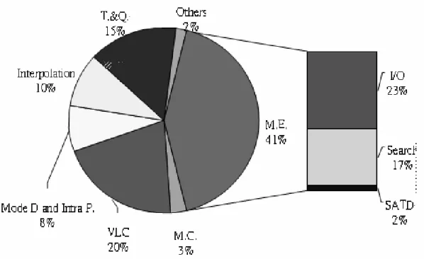
The H.264 encoder reference software provided by the ITU/MPEG standard committee is known for its high computational complexity. A typical computational profile of the H.264 encoder (ITU/MPEG reference software) running on Intel PC, is shown in Fig 2. It shows that the tools of (a) motion estimation, (b) entropy coding, (c) transform and quantization, (d) interpolation, and (e) mode decision and intra-prediction are the most time-consuming modules. Although the other results of profiling would have somewhat different, by and large, the trend is pretty much the same. As for the decoder, the tools of (a) motion compensation (including interpolation), (b) entropy decoding, and (c) intra-prediction have the CPU load.
2.2 INTRA PREDICTION 2.2.1 Overview
Intra-prediction uses the high correlation property of neighboring samples in spatial domain to predict the current encoded samples. For the luma samples, each prediction block may be formed for each 4x4 block (denoted as I4MB) or for an entire MB (denoted as I16MB). When utilizing Intra_4x4 prediction, each 4x4 block chooses one of the nine prediction modes, which include one DC mode plus eight directional prediction modes, as shown in Fig 3 (a), as the best one. In the luma component of an MB, the Intra_16x16 prediction is typically chosen for smooth image areas, and thus, only four prediction modes are specified as shown in Fig 3 (b) except for the DC mode. The chroma samples of an MB are predicted using a similar prediction pattern, Intra_8x8, which is similar to the luma Intra_16x16 prediction.
(a) (b)
Fig 3 Intra prediction modes for (a)Intra_4x4 and (b) Intra_16x16.
2.2.2 Fast algorithms
The fast algorithms of intra prediction can be classified into several types. The first approach is “early termination”, which ends the search operation when the calculated distortion is samller than a pre-chosen threshold. The selection of a proper measure for deciding termination is critical to the performance. It may be derived based on the macroblock smoothness [6][7] or the most probable mode [8]. The early termination based on the macroblock smoothness calculates a smoothness measure of a macroblock to determine the block type. For example, the large block type such as Intra_16x16 is chosen often for the flat image areas [6][7]. “Smooth” means that all the pixel values in a MB are similar; that is, their variance is small. The variance computation shall be simple to save computation. Therefore, the Mean Absolute Difference (MAD) operation [6] or the AC/DC ratio [7] is often used. If the variable is
smaller than a pre-selected threshold value, the Intra_16x16 mode is chosen and thus the costly Intra_4x4 can be skipped.
Another kind of early termination proposal examines the most probable mode first. For example, in searching for the best Intra_4x4 mode, if its residual is smaller than a threshold, then the other eight Intra_4x4 modes are skipped (not chosen). Otherwise, all nine modes have to be tested. Then, we set another threshold to decide whether to keep on checking the Intra_16x16 prediction or not. It was reported that in one case, this method together with the 2:1 downsampling and rate-distortion optimization (RDO) can reduce 68.8% of total computation time with only 1.35% of bit rate increase comparing to the reference software [8]. The major issue in this type of algorithms is how to determine the threshold. The threshold value can be adjusted according to the quantization parameters for instance. To construct a more efficient scheme, we propose a mixed fast intra prediction algorithm. It first examines both the most probable mode and the DC mode to determine if it meets the early termination criterion. The threshold value is decided by the average of SATD (sum of absolute transformed difference) of all the previous Intra_4x4 blocks in this frame. Once the 16 Intra_4x4 blocks are done, their total cost will be used as the threshold for deciding Intra_16x16 mode. These threshold values seem to be able to match the video local characteristics and provide good results. Even when RDO is turned off, we can achieve around 30% computational savings for the intra prediction module.
The second approach uses the edge analysis to quickly identify the edge direction since the intra prediction is basically a directional prediction [9][10]. Often the Sobel operators or the first order derivative are used as the edge analysis tool to find the most probable edge, which will be used as one of the final edge candidates. The final mode candidate list includes the one selected by the edge detector together with the other highly probable modes. In the case Intra_4x4, this would mean two modes of the neighboring blocks and the DC mode; and in the Intra_16x16 and Intra_8x8 cases, only the DC mode is considered highly probable. Therefore, only four candidate modes (for Intra_4x4) or two candidate modes (other types) are needed to be examined. The result shows that 60% of intra_only computation time reduction is observed with RDO and the bit rate increase is around 2~3% [9]. The bit rate increase may be owing to the irregular edges within a block. On the other side, the extra computation needed for edge analysis can be a computation burden and reduce the overall saving significantly.
horizontal and vertical directions, it then tests the neighboring 22.5 degree modes close to the better one from the previous step, and finally the best mode up-to-now is checked against the DC mode for the final winner. This approach has the advantage of a fixed number of modes are examined for all cases. However, computation time reduction is around 33% with about 1% bit rate increase.
The last approach makes use of the correlation in the temporal domain [12] since the best prediction mode in the current macroblock is likely similar to that in the reference macroblock in the previously coded frame(s). Thus, the primary intra prediction mode is selected from the mode of the most overlapped block in motion estimation. The computational overhead is nearly zero since all information is obtained during the inter-prediction operation. It is reported that the coding performance is nearly unchanged while the computational savings is about 50% assuming the intra-frame period is 10 [12].
In summarizing various fast intra-prediction algorithms, although we cite the experimental results from the proposed documents, a fair comparison among all methods is difficult because their simulation environments are quite different. One important element affecting computation is the option of RDO in the reference software. This is particularly true for the early termination method with thresholds. The algorithms described in the above can be combined together to achieve further speed-up. For example, the first step could be the decision on Intra_4x4 or Intra_16x16. The second step could be the early termination for the chosen intra type. Finally, the rest of mode tests could be a fast algorithm to select one from the nine or four candidate modes.
2.3 INTER PREDICTION 2.3.1 Overview
Block matching based motion estimation and compensation is a fundamental process in the current international video compression standards. It can efficiently remove interframe redundancy. A direct implementation is the full search algorithm that examines exhaustively every candidate motion vector in the search window to find the globally best matched block in the reference frame. However, its computationally intensive nature prevents it from practical implementation on a processor for real-time applications. The computation burden is increased drastically for the H.264 encoder because there are a number of combinations of partitioning a macroblock into sub-block(s) ranging from 4x4 to 16x16. Potentially each sub-block can have its own motion vector. This feature significant increases the computational complexity in motion estimation. Thus, many fast motion estimation algorithms have been proposed to alleviate the computational load.
Most of the fast algorithms are based on the well-known a priori knowledge, “the motion field of a real world image sequence is usually gentle, smooth and varies slowly”. Fast motion estimation algorithms can be categorized into roughly three families as described below.
2.3.2 Fast algorithms
2.3.2.1 Reduce possible candidate points
(a) (b)
Fig 4 (a) S. Zhu and K.-K. Ma, “A new diamond search algorithm for fast block matching motion estimation”,[19]. (b) C. Zhu, X.
Lin,and L.–P. Chau, “Hexagon-based search pattern for fast block motion estimation,[21]
Based on the assumption of convexity of the uni-modal error surface, i.e., block matching distortion increases monotonically away from the global minimum point, many gradient-based search methods with carefully designed search patterns have been developed to limit search points to a small subset of all possible candidates. This category includes the well-known three-step search (3SS) [13], the new three-step search (N3SS) [14], the cross search (CS) [15], the one-dimensional gradient descent search (1DGDS) [16], the block-based gradient descent search (BBGDS) [17], the four-step search (4SS) [18], the diamond search (DS) [19], the cross-diamond search (CDS)[20] and the hexagon-based search (HEXBS) [21]. Although this category of algorithms may be trapped into a local minimum point and hence the efficiency of the motion compensation may drop, they can considerably reduce the number of block matching computations.
2.3.2.2 Motion vector prediction NR MV uuuuuuv ' t t' 1+ _ ' ' 1 pred NRP NR t t MV MV t t − = × − − uuuuuuuuuuuv uuuuuuv
Fig 5 Temporal Neighboring Ref-frame Prediction
Fig 6 Spatial Up-Layer Prediction
Motion in most natural image sequences involves a few blocks and lasts for a few frames. Therefore, spatially or temporally adjacent blocks often have similar motion vectors. Taking the advantage of the correlation among neighboring motion vectors, the search window can be constrained to a small clique surrounding the “predicted vector”, a candidate position predicated based on the known neighboring motion vectors. Many prediction algorithms have been developed with different complexities. The prediction search algorithm (PSA) [22] simply predicts the current block motion vector as the mean value of its neighboring blocks’ motion vectors. Fuzzy search [23] applies fuzzy logic to predict the motion vector. In [24], motion vectors are predicted by integral projections. In [25], a spatial-temporal AR model of motion vectors is constructed and an adaptive Kalman filter is employed. The multi-resolution search [26] down-samples a picture to obtain raw motion vectors at different resolution levels, then it estimates finer motion vectors from the coarser ones.The multi-resolution-spatiotemporal (MRST) scheme [26] modifies the normal
raster scan order so that some blocks can reference more motion information by increasing their neighboring blocks along more directions. It then combines a multi-resolution scheme and spatiotemporal correlation to predict motion vectors. For burst motions and blocks at the top-left corner, which has little correlation information, the performance of this category of algorithms may deteriorate because the refinement of prediction is restricted to a small search region. Moreover, the prediction overhead may reduce the speed gain.
2.3.2.3 Low complexity block matching criteria
The majority of the computations in motion estimation originate from computations of block matching distortion. In general, block matching metrics, such as the mean absolute difference (MAD) and the mean square error (MSE), involve pixel-wise operations, which are highly computationally intensive. Some methods try to simplify distortion computation by substituting the distortion defined on a subset of pixels for the whole block distortion. For instance, the MAD of 128 pixels is used as the matching distortion for a 16x16 macroblock in [26]; the computations can be reduced by one half with little performance loss. However, this method is not suitable for small blocks such as 4x4 blocks. Partial distortion elimination (PDE) in [27] compares every line’s distortion in a block to avoid computing the distortion of the entire block. In [28], hypothesis testing is used to estimate the MAD from the partial mean absolute difference (PMAD), and the estimated MAD value is used to judge the matching result.
When fast algorithms in the above three categories are put together, the motion estimation accuracy may degrade. Additional calculations such as the initial motion vector prediction could lead to a considerable amount of computational overhead. An approach proposed without quality degradation is the successive elimination algorithm (SEA) suggested by Li and Salari [29], which pre-excludes some impossible candidate points before completing the matching distortion calculation. SEA is a fast full search algorithm having a performance identical to FS while it speeds up the search process approximately by 10 times for 16x16 macroblock based motion estimation. Some further improvements have been made in subsequent research [27][30]-[33].
2.3.2.4 Fast fractional motion estimation
(a) (b)
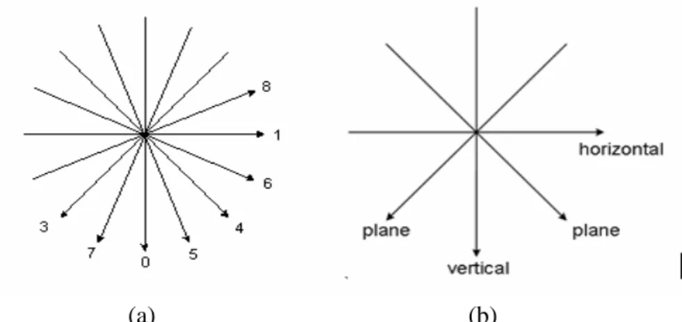
Fig 7 (a)H.-M. Wong, O. C Au, and A. Chang, “Fast sub-pixel inter-prediction–based on the texture direction analysis”, [35](b)
C.-C. Cheng, Y.-J. Wang, and T.-S. Chang, “A fast fractional pel motion estimation algorithm for H.264/AVC”,[36].
In the H.264 video coding scheme [4], the inter prediction (motion vectors) precision has been increased to quarter pixel. Typically, people perform the integer pixel motion estimation (IME) first. Then, the sub-pixel motion estimation or fractional motion estimation (FME) is applied to achieve refinement. As compared to the integer-value search, FME has a somewhat different statistical character. This may due to the facts that the search window of FME refinement is much smaller than that of IME and that the referenced sub-pixels are interpolated from the integer-coordinate pixels. Consequently, the error surface of FME is much closer to a uni-modal one, which favors fast algorithms.
Therefore, traditional fast algorithms in IME can also be used and can be more effective. The scheme adopted by the H.264 reference software is a three-step-like fast algorithm. It first checks the nine candidates surrounding the best match of IME, and then checks further the nine candidates surrounding the best match from the previous step. However, to take even more advantage of the uni-modal surface property and the highly centralized distribution of sub-pixel motion vectors, several fast FME algorithms with additional features are proposed. In [35], a gradient based search algorithm is brought up. The search direction is determined first and looks for the best motion vector along that direction. In [36], an adaptive search-pattern algorithm is proposed. The search-pattern is determined by outcome of the previous step and it biased towards the search center. This method saves half of the computations when compared to the reference software.
2.3.2.5 Some recent approaches
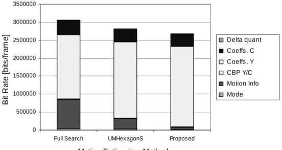
The recent trend to further reduce the motion estimation calculations is to combine the techniques mentioned before. The idea is each technique, a fast algorithm, is placed its most suitable target area. Thus, how to find a specific combination that achieves the optimal solution for a specific application becomes the most important issue. In [37], a fast algorithm with better coding efficiency on residuals is proposed, which leads to a lower bit rate compared to the full search algorithm. The method proposed in [38] produces larger residuals (due to fewer search points) but less motion information. Overall, it has a better encoding efficiency and a rather fast coding speed. This type of solutions seems to the target now researchers are aiming at.
0 500000 1000000 1500000 2000000 2500000 3000000 3500000
Full Search UMHexagonS Proposed
Motion Estimation Methods
B it R a te [bi ts /fr am e ] Delta quant Coeffs . C Coeffs . Y CBP Y/C Motion Info Mode
2.4 FAST MODE DECISION 2.4.1 Overview
The mode decision algorithm determines the best mode of the macroblock from various combinations of inter-prediction and intra-prediction. It can be coded with seven different block sizes for motion-compensation in the inter mode, and various spatial directional prediction modes in the intra mode. To achieve the highest coding efficient as close as possible, the reference software calculates the rate distortion costs of all possible modes and the it chooses the best one that has the minimum cost. This is a very time-consuming process. To reduce the computation load, a fast mode decision algorithm is necessary, which can do a quick screening to drop most poor modes and then it examines the reminders and identifies the (nearly) best one.
2.4.2 FAST ALGORITHMS
The fast mode decision algorithm can be divided into two types. The first type uses an early termination threshold to terminate the lengthy mode decision process. The early termination step can be placed between the intra and inter prediction processes [43][44] or inside the inter prediction process [45].
The scheme proposed in [43][44] uses the fact that intra mode needs more bits for coding and thus has a lower priority than the inter mode. Thus, if the best inter mode cost is smaller than a threshold, the intra prediction mode is skipped. The threshold can be the average of rate distortion cost of a number of previously coded intra blocks [43] or a ratio between the average boundary error (ABE) and average rate (AR) [44], where AR is the average bits for encoding the motion-compensated residuals and ABE is the average pixel error between the pixels at boundary of the current and its adjacent blocks in the best inter mode. The simulation results show that it can achieve about 20% reduction of computational time with a slight bitrate increase.
In [45], it observes the fact that the 16x16 block usually is the best block size for large areas of background with still or uniform motion since it has less motion vector overhead. Thus, it first checks the cost of 16x16 block size. If it is smaller than a threshold, say, an average value of previous 16x16 blocks, the inter prediction process is terminated. Otherwise, a similar procedure is applied to the 8x8 block size. The second type of the mode decision algorithms is to reduce the number of candidate modes. Intuitively, if the cost of a larger block-size mode is higher than the cost of the
current block-size mode, the even larger block-size modes can be excluded. Similarly, if the cost of a smaller block-size is higher than that of the current block-size mode, the even smaller block-size modes can be excluded. Following this argument, we give different priority to each mode. If the mode with higher priority can provide sufficient image quality, we can skip the other lower priority modes. A specific case is the SKIP mode. The SKIP mode refers to the 16x16 mode of which no motion and residual information is coded. Thus, no motion search is required and it has the lowest complexity. Therefore, many algorithms assign the highest priority to the SKIP mode and thus a large percentage of macroblocks would get the SKIP mode based on spatial-temporal neighborhood information [46]-[48]. This approach can save a significant proportion of the encoding time with a slightly bit rate increase and quality drop.
In summary, the fast mode decision algorithms can be combined with the other fast intra and inter prediction algorithms to achieve further speedup. In all these algorithms, the SKIP mode first approach can save significant computational time. How to determine proper threshold values in a simple and automatic way is one critical issue for research and many proposals have been suggested.
Chapter 3
Dynamic search range prediction
for integer motion estimation
3.1 DESCRIPTION OF PRIOR ART
Motion estimation is a well known technique in video coding to achieve high coding efficiency by reducing the temporal redundancy between successive frames. Motion estimation plays an important role in such an inter-frame predictive coding system.
The full search block matching algorithm for motion estimation is the simplest but computationally very intensive, especially when the search range is large. It provides an optimal solution by exhaustively evaluating all the possible candidates within the search range in the reference frame. Many fast algorithms, such as the new three-step search [14], the block-based gradient descent search [17], the three-step search [39], the dynamic search window scheme [40], and one-at-a-time search [41] have been proposed to reduce the computational complexity by limiting the number of check points within the constant search range. The basic idea behind there fast algorithms is the assumption of the monotonically increasing block distortion function. Limited points are tested in the first stage; search is then continued in the vicinity of the point whose distortion is the smallest in previous stage. In [40], the window size in subsequent stage is determined based on the superiority of the best matched point to others in the present stage. It is clear that all these algorithms start with a constant search range and the computational complexity reduction is done at the expense of estimation accuracy due to its limited number of check points in the first stage. Different approached of fast algorithms have also been proposed. In [42], the sub-sampled motion-field estimation scheme is proposed. It starts with sub-sampled motion-field estimation and then selectively replicates it to produce all the motion vectors. However, it performs poorly when two or more objects within the same block are moving in different directions or different velocities [42].
3.2 ANALYSIS OF INTEGER MOTION VECTOR
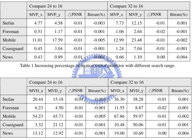
performance increasing rate will saturate until certain degree video quality has been achieved. In order to make the compress process more efficient, we may need to know the saturate boundary of the input search range. The factor straight affected by changing input search range is motion information. Motion vector can be decomposed of motion vector predictor and motion vector difference. In Table 1, we can find the increasing rates of motion vector predictor are really small compare to the increments of input search range. For the reason that comparisons from 32 to 16 are very similar as that from 24 to 16, we can easily conclude that the increment of input search range over the saturate boundary will not get better coding efficiency.
Compare 24 to 16 Compare 32 to 16
MVP_x MVP_y △PSNR Bitrate(%) MVP_x MVP_y △PSNR Bitrate(%)
Stefan 4.77 4.58 -0.01 -0.003 7.73 12.15 -0.01 0.001 Foreman 0.51 1.17 -0.01 -0.001 1.06 2.64 -0.02 -0.001 Mobile 11.01 17.59 -0.01 -0.005 12.99 23.48 -0.01 -0.002 Coastguard 0.45 3.04 -0.01 -0.001 1.24 7.04 -0.01 -0.001 News 0.43 0.89 -0.01 -0.001 0.66 1.10 0.00 -0.004
Table 1 Increasing percentage of motion vector predictor with different search range. Compare 24 to 16 Compare 32 to 16
MVD_x MVD_y △PSNR Bitrate(%) MVD_x MVD_y △PSNR Bitrate(%)
Stefan 20.44 15.18 -0.01 -0.003 36.30 38.28 -0.01 0.001 Foreman 6.23 4.50 -0.01 -0.001 11.55 8.87 -0.02 -0.001 Mobile 54.23 45.73 -0.01 -0.005 67.86 59.97 -0.01 -0.002 Coastguard 3.32 21.12 -0.01 -0.001 10.48 50.06 -0.01 -0.001 News 13.12 12.92 -0.01 -0.001 19.00 10.60 0.00 -0.004
Table 2 Increasing percentage of motion vector difference with different search range.
In Table 2, the same conclusion can be epitomized. Motion vector difference shows larger increasing rate with comparison to motion vector predictor, but it still not efficient enough when input search range is too large. To determine whether the input search range is too large or not, we experimented the input sequence size as CIF size to find the saturate boundary of input search range for every input sequence respectively.
As shown in Table 3, critical search range means the smallest search range with similar rate distortion performance. We listed all possible factors that will announce the search range needed. The factors that we considered can mainly be divided into
two families: matching error group and motion information group. In the former group, we record not only sum of absolute difference (SAD) but also sum of absolute transformed difference (SATD); in the later group, we record motion movement information. It is generally believed that temporal and spatial correlations of motion vector exist. As the result, it gives us spaces to apply fast algorithm.
Critical SR SAD SATD MVP_x MVP_y MVD_x MVD_y Stefan 8 303.34 381.88 23.86 4.22 1.37 0.40
Foreman 4 176.64 267.79 17.51 6.51 0.66 0.55
Mobile 4 408.33 500.96 17.15 3.85 0.96 0.43
Coastguard 2 276.61 436.79 19.21 2.33 0.70 0.08
News 2 122.55 197.70 13.57 4.12 0.12 0.11
Table 3 The correlation between search range and the factors including matching error and motion information. Critical search range means the smallest search range with similar RD performance.
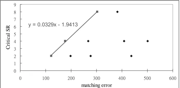
y = 0.0329x - 1.9413 0 1 2 3 4 5 6 7 8 9 0 100 200 300 400 500 600 matching error C ritic a l S R
Fig 9 Correlation between critical search range and matching error.
The correlation of critical search range and factors mentioned in Table 3 are very similar. Taking matching error as the example, when the x coordinates (matching error) are getting larger, the y coordinates (critical search range) are not getting larger proportionally. In Fig 9, we can obviously find that when the matching error too small or too large have smaller critical search range. To examine the reason, it is very straight forward that too small matching error has smaller critical search range. As the belief of the spatial correlation, slight motion movement (usually small matching error) in previous macroblock means probably slight motion movement in current macroblock. To cover the slight motion movement, only small critical search range is
needed. In the case of larger matching error, it usually means that we can not find a good match position in the search window such as changing scene or complex texture within the macroblock. Indeed even if we increase the input search range will have very little RD performance improvement. As the result that motion estimation does not compress the macroblock information with large matching error, we may want to reduce the search range to achieve our goal as speedup.
3.3 PROPOSED ALGORITHM
A fast algorithm for motion estimation is proposed in this chapter. In contrast to previously proposed fast algorithms which use limited number of check points in a constant search range. The proposed algorithm performs search in a dynamic search range.
Block motion fields in real world video sequences are usually smooth and varies slowly. This produces a high correlation between the motion vectors of neighboring blocks. We record the matching error of the previous macroblock. By making use of this information, we will determine the search range used in current macroblock dynamically. The proposed algorithm can mainly divided into three steps. The details are as follows:
Step 1: Predict search range.
If (qp > 30)
qp_factor = 2; else
qp_factor = 1;
sr_factor = (input->search_range)>>4; shift_factor = qp_factor + sr_factor;
To serve different resolution video content, we should adjust the predict scheme dynamically. Two main factors result in different resolution are quantization parameter and input video size. The former one let users can define the final video quality according to their application. The later one let users can compress video content with different input size such as QCIF for network streaming and D1 for DVD player. As the different input size, the different input search range comes. In order to reduce the error generate by predicting search range, we should adjust the sr_factor dynamically.
Mvd_max = ( |mvd_x_prev| , |mvd_y_prev| ); max_sr = Mvd_max << shift_factor;
We record the motion vector difference of the previous macroblock for the reason that correlation exists. It is generally believed that motion vector is likely
similar as the previous one. However, this is not point motion vector difference directly. We may know the entire motion vector likely is but we can not judge the refined part (motion vector difference) accurately, so Mvd_max need to be increased to generate the probable predict search range (max_sr).
Step 2: Check the upper bound.
if(sad_previous > 600) max_sr_up = (search_range >> 2); else if(sad_previous > 50) max_sr_up = search_range; else max_sr_up = (search_range >> 1);
max_sr = min (max_sr, max_sr_up);
In this step, we want to clip some redundant search range that was over predicted in previous step. The main idea is cut off the search range when the match error is too large or too small. The correlation is shown in Fig 9 and details are mentioned above. 600 and 50 are experiment result with input sequence as CIF size. Bad match (with too large matching error) shows more spaces to reduce search range than good match (with too small matching error) does. When matching error is over 600, it means that there is no good match position in search window. In other words, even if we skip the motion estimation process, it will not result in terrible performance loss. The amount of residual data can not be saved, so spending time to refine motion vector is not efficient and can be reduced.
Step 3: Check the lower bound.
if(max_sr == 0) max_sr = 4;
The last step is to avoid skipping motion refined operation. In this step, we will make sure that the max_sr is not equal to zero. The action that skipped motion refined operation will lead to significantly rate distortion performance loss.
3.4 COMPARISON
This section shows the speedup improved by proposed fast algorithm. Saving mentioned below means the reduced search points compared to original ones. We record every determined search range in all macroblocks and calculate the average of them. Saving is calculated manually. It means not the total encoding time saving but motion refinement time saving. As listed in Table 4, the input sequence size is CIF size and input search range is given by 16. We find that the proposed algorithm obviously decreases the number of search points. When the quantization parameter is smaller than 30, almost 90% saving can be achieved. It still has more than 80% saving even the quantization parameter is bigger than 30.
QP=20 QP=24 QP=28 QP=32 CIF
SR=16 Sr_avg Saving(%) Sr_avg Saving(%) Sr_avg Saving(%) Sr_avg Saving(%)
Stefan 6.764 82.126 6.753 82.184 6.663 82.652 7.915 75.528 Mobile 4.573 91.828 4.544 91.931 4.464 92.213 6.453 83.732 Foreman 5.665 87.462 5.704 87.287 5.676 87.410 7.335 78.978 Coastguard 4.699 91.373 4.745 91.204 4.790 91.034 6.639 82.778 News 4.365 92.555 4.391 92.465 4.391 92.468 4.758 91.154 Average 89.069 89.014 89.156 82.434
Table 4 saving statistic with input search range = 16 and input sequence size as CIF size.
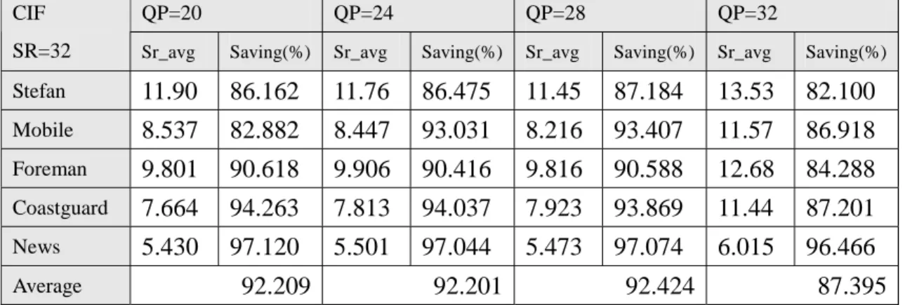
QP=20 QP=24 QP=28 QP=32 CIF
SR=32 Sr_avg Saving(%) Sr_avg Saving(%) Sr_avg Saving(%) Sr_avg Saving(%)
Stefan 11.90 86.162 11.76 86.475 11.45 87.184 13.53 82.100 Mobile 8.537 82.882 8.447 93.031 8.216 93.407 11.57 86.918 Foreman 9.801 90.618 9.906 90.416 9.816 90.588 12.68 84.288 Coastguard 7.664 94.263 7.813 94.037 7.923 93.869 11.44 87.201 News 5.430 97.120 5.501 97.044 5.473 97.074 6.015 96.466 Average 92.209 92.201 92.424 87.395
Table 5 saving statistic with input search range = 32 and input sequence size as CIF size.
In Table 5, we see the similar result with different simulation environment. We get even better result than that shown in Table 4. As the total encoding time issue, when the search range is larger, the time spending on motion estimation occupies bigger portion of total encoding time. So we can achieve 40% ~ 60% total encoding time saving with input search range given by 16 but 60% ~ 80% total encoding time
saving with input search range given by 32.
QP=20 QP=24 QP=28 QP=32 D1
SR=32 Sr_avg Saving(%) Sr_avg Saving(%) Sr_avg Saving(%) Sr_avg Saving(%)
Crew 17.23 70.984 15.85 75.452 14.43 79.653 16.21 74.311
Harbour 12.54 84.633 11.91 86.144 11.07 88.031 13.51 82.153
Might 13.48 82.239 12.91 83.718 12.43 84.890 13.97 80.922
Sailormen 14.93 78.203 13.97 80.927 13.10 83.239 17.45 70.237
Average 79.015 81.560 83.953 76.906
Table 6 saving statistic with input search range = 32 and input sequence size as D1 size.
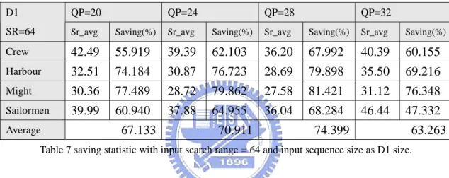
QP=20 QP=24 QP=28 QP=32 D1
SR=64 Sr_avg Saving(%) Sr_avg Saving(%) Sr_avg Saving(%) Sr_avg Saving(%)
Crew 42.49 55.919 39.39 62.103 36.20 67.992 40.39 60.155
Harbour 32.51 74.184 30.87 76.723 28.69 79.898 35.50 69.216
Might 30.36 77.489 28.72 79.862 27.58 81.421 31.12 76.348
Sailormen 39.99 60.940 37.88 64.955 36.04 68.284 46.44 47.332
Average 67.133 70.911 74.399 63.263
Table 7 saving statistic with input search range = 64 and input sequence size as D1 size.
In order to make the method suitable for all kinds of video content, we concerned about many factors and adjusted the prediction scheme respectively. We developed the algorithm with input sequence size as CIF size. As shown in Table 6 and Table 7, we took input sequence size in D1 size as an experiment. The results show that smaller saving comes with larger input sequence size. It means that the proposed algorithm is a little conservative for larger input sequence size. Even if the determined search range is over predicted, it still has almost 80% saving as listed in Table 6 and almost 70% saving as listed in Table 7. As the total encoding time issue, both of them are about 40% ~ 60% saving.
3.5 SIMULATION RESULT
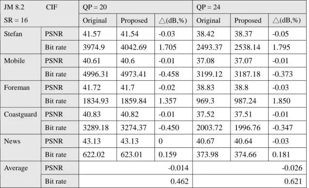
After the comparison of the speedup, this section shows the corresponding rate distortion performance. We summarized the result into Table 8 to Table 11. We have less than 0.03 dB PSNR drop and less than 0.5 % bit rate increased in the case of input sequence size as CIF size (Table 8 and Table 9).
QP = 20 QP = 24 JM 8.2 CIF
SR = 16 Original Proposed △(dB,%) Original Proposed △(dB,%) PSNR 41.57 41.54 -0.03 38.42 38.37 -0.05 Stefan Bit rate 3974.9 4042.69 1.705 2493.37 2538.14 1.795 PSNR 40.61 40.6 -0.01 37.08 37.07 -0.01 Mobile Bit rate 4996.31 4973.41 -0.458 3199.12 3187.18 -0.373 PSNR 41.72 41.7 -0.02 38.83 38.8 -0.03 Foreman Bit rate 1834.93 1859.84 1.357 969.3 987.24 1.850 PSNR 40.83 40.82 -0.01 37.52 37.51 -0.01 Coastguard Bit rate 3289.18 3274.37 -0.450 2003.72 1996.76 -0.347 PSNR 43.13 43.13 0 40.67 40.64 -0.03 News Bit rate 622.02 623.01 0.159 373.98 374.66 0.181 PSNR -0.014 -0.026 Average Bit rate 0.462 0.621
Table 8 rate distortion result with input search range = 16 and input sequence size as CIF size. QP = 20 QP = 24
JM 8.2 CIF
SR = 32 Original Proposed △(dB,%) Original Proposed △(dB,%)
PSNR 41.59 41.55 -0.04 38.45 38.4 -0.05 Stefan Bit rate 3907.46 3931.66 0.619 2414.45 2445.22 1.274 PSNR 40.6 40.59 -0.01 37.08 37.06 -0.02 Mobile Bit rate 5016.42 4983.1 -0.664 3212.55 3190.48 -0.686 PSNR 41.72 41.7 -0.02 38.83 38.8 -0.03 Foreman Bit rate 1837.43 1854.24 0.914 970.15 983.24 1.349 PSNR 40.83 40.82 -0.01 37.52 37.51 -0.01 Coastguard Bit rate 3296.59 3279.85 -0.507 2006.07 1997.74 -0.415 PSNR 43.14 43.12 -0.02 40.67 40.63 -0.04 News Bit rate 624.8 627.92 0.499 375.32 378.82 0.932 PSNR -0.02 -0.03 Average Bit rate 0.172 0.490
Table 9 rate distortion result with input search range = 32 and input sequence size as CIF size.
The previous section have pointed out that the speedup of the larger input sequence size has less speedup. In other words, less speedup means better rate distortion performance. The argumentation can be proved in this section through Table 10 to Table 11. We can find that both PSNR drop and bit rate increased are obviously smaller than that in Table 8 and Table 9.
QP = 20 QP = 24 JM 8.2 D1
SR = 32 Original Proposed △(dB,%) Original Proposed △(dB,%) PSNR 41.97 41.95 -0.02 39.34 39.33 -0.01 Crew Bit rate 9727.04 9611.98 -1.182 4935.23 4896.6 -0.782 PSNR 41.22 41.19 -0.03 38.28 38.26 -0.02 Harbour Bit rate 13516.99 13176.58 -2.518 8157.34 7999.64 -1.933 PSNR 41.97 41.95 -0.02 39.1 39.08 -0.02 Night Bit rate 10574.44 10446.64 -1.208 5740.23 5712.69 -0.479 PSNR 41.04 41.02 -0.02 38.01 38 -0.01 Sailormen Bit rate 12398.86 12267.2 -1.061 5955.03 5920.67 -0.576 PSNR -0.022 -0.015 Average Bit rate -1.492 -0.943
Table 10 rate distortion result with input search range = 32 and input sequence size as D1 size. QP = 20 QP = 24
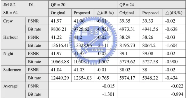
JM 8.2 D1
SR = 64 Original Proposed △(dB,%) Original Proposed △(dB,%) PSNR 41.97 41.96 -0.01 39.35 39.33 -0.02 Crew Bit rate 9806.21 9725.62 -0.821 4973.31 4941.56 -0.638 PSNR 41.22 41.2 -0.02 38.29 38.26 -0.03 Harbour Bit rate 13616.41 13328.96 -2.111 8195.73 8064.2 -1.604 PSNR 41.97 41.95 -0.02 39.1 39.08 -0.02 Night Bit rate 10663.88 10503.1 -1.507 5779.62 5727.58 -0.900 PSNR 41.04 41.03 -0.01 38.02 38 -0.02 Sailormen Bit rate 12449.29 12354.03 -0.765 5974.17 5948.22 -0.434 PSNR -0.015 -0.022 Average Bit rate -1.301 -0.894
Table 11 rate distortion result with input search range = 64 and input sequence size as D1 size.
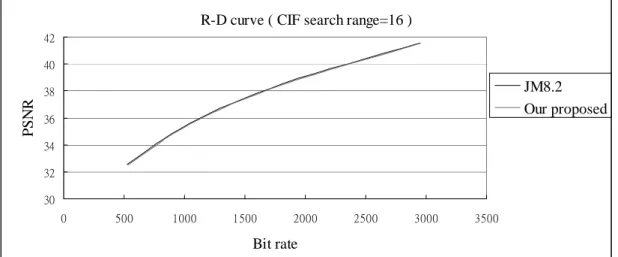
We have less than 0.022 dB PSNR drop and even lower than original bit rate performance. When the quantization parameter is getting bigger, the less coding efficiency is carried with. However, in order to get so huge a speedup, sacrificing small amount of quality loss is still worth. Rate-distortion curves are shown in Fig 10 and Fig 11. As the input sequence as CIF size, we simulated search range equal to 16 and 32; as the input sequence as D1 size, we also simulated search range equal to 32 and 64. All of them are very close to original method.