Effects of the quantum size and an off-center donor atom on energy levels in a quantum dot

CHINESE JOURNAL OF PHYSICS VOL. 36, NO. 4 AUGUST 1998

Effects of the Quantum Size and an Off-Center Donor Atom on Energy Levels in a Quantum Dot

Jone-Zen Wang and Tzong-Jer Yang

Department of Electra-physacs, National Chiao-Tung University, Hsinchu, Taiwan 300, R.0.C

(Received February 20, 1998)

Gorecki and Brown [J. Phys. B 22, 2659 (1989)] proposed a variational theory for the ground state. They assumed the trial wave function in confined systems as f4, where f acted as a variable contour function to minimize the energy. In practical calculations, it is only possible to calculate electronic energy levels at some shapes off to decide which f gives the minimal energy. Due to this constraint in the variational calculation of f, their method gives unsatisfactory results in asymmetrical quantum problems, and therefore is rarely used. We generalize their method by assuming the trial wave function as f$~, where $ is a linear combination of basis functions. In our improvement, the use of the linear combination of basis functions acts not only to simulate efficiently the asymmetrical state but also to the give energy levels of the excited state. For the same reason, our method can be applied in open systems and in the problem where a new potential exists. Therefore, the goal of our improvement is to propose a general variational method. As applications, the changes of binding energies and donor states in spherical and ellipsoidal semiconductor quantum dots are studied when the position of the donor is shifted and when the size of the dot is changed. PACS. 71.15-m - Methods of electronic structure calculations.

PACS. 71.55-i - Impurity and defect levels. I. Introduction

The advances in crystal-growth techniques such as molecular-beam epitaxy (MBE) and metalorganic chemical vapor deposition (MOCVD) h ave accelerated the researches in microstructures, such as quasi-two-dimensional (Q2D) quantum wells, quasi-one-dimensional (QlD) quantum-well wires and quasi-zero-dimensional (QOD) quantum dots. The experi-mental techniques used to provide three-dimensional confinement for QOD systems were not mature until recent years, therefore QOD problems have been received much experimental and theoretical .attention [l-5].

Because the coordinate variables do not separate and there have been difficulties in satisfying the boundary conditions in most QOD (also for Q2D and QlD) systems, approx-imation methods should be used. Unfortunately, there is not a general variational method to provide systematic approaches on electronic states in these problems. The conventional variational methods usually deal only with the ground state and are difficult to apply to systems of low symmetry. This fact allows the theoretical investigations only in highly

6 1 7 @ 1998 THE PHYSICAL SOCIETY OF THE REPUBLIC OF CHINA

618 EFFECTSOFTHEQUANTUMSIZEANDANOFF-CENTER... VOL.36

systems, like spherical or cubic quantum dots. To obtain a more realistic realization of the electronic structures in these problems, we need a general variational method to solve the Schrodinger equation.

In the work of Gorecki and Byers Brown (GB) [6], they proposed a new variational method whose solutions can completely obey the boundary condition in the quantum sys-tems with infinite potential walls. Their theory treated only the ground state and the trial function was assumed as

4 = f40,

(14

where f is a contour function which vanishes at the infinite potential wall and 40 is the ground state wavefunction of the quantum system without the infinite potential wall. When the $0 is a nodeless function such a trial function 4 = f$u is a reasonable assumption. If the contour function f can be varied in any shape to minimize the ground state energy, this method is a general variational scheme. However, it is impossible to change the shape of f arbitrarily in practical calculations. Therefore, its applications in asymmetrical quantum systems[6,7] demonstrate apparently the lower numerical accuracy because of the contour function less matching the real situation. Due to this fact, this method is seldom used.

In our generalization of the method of GB, we assumed the trial function as

4 = f

Cai4i7

i

(1.2)

where 4; are eigenstates of the quantum system without the infinite potential wall. The linear combination of basis functions can effectively simulate the symmetric property of any quantum system, if the number of basis functions is large enough. Therefore, such a trial function compensates the drawback that the shape of the contour function can not be changed arbitrarily in practical calculation. Besides, because of the use of basis functions, properties of excited states are calculated and energy states in those problems where new potentials exist can also be simulated in our new scheme. These facts make our method a really general variational method. The variational parameter oi and contour function f need to be determined in the variational calculation. So, the steps in our calculations are more complicated than those in the work of GB.

The rest of this work is organized as: In sec. II, we describe the formulation in our method. In sec. III-l, donor states in a spherical quantum dots are calculated to check the accuracy of our new method. The results match well with exact data or data from other work. Compared with the work of GB, the improvement in our results is apparent. In sec. 111-2, we systematically calculate and compare the data of donor states in ellipsoidal and spherical dots when the size of dots is changed and when the position of the donor is shifted from the center.

II. Calculation method

In this section we will present the theoretical formulation of our new variational method. Let us consider a general quantum system with the Hamiltonian as

~~ = - ; A + U(:),T E R”,

₍₂₄

VOL. 36 JONE-ZEN WANG AND TZONG-JER YANG 619

where A denotes the Laplacian operator in R” . We assume the eigenstates of Hn beeing written as $i, i = 0,1,2,. . ., where 40 is the ground state. The Schrodinger equation reads

(2.2)

Then let us consider the same quantum system, but enclosed in the space region 0. The Hamiltonian becomes

H =

-;A

t

U(z) + v(y)

(2.3)

where

V(Z) = 0,a:E R

CO,?? $$R. (24

The purpose in such a quantum mechanic problem is to find out the eigenstates of H, which satisfy

(2.5)

Unfortunately, the eigenvalue equation (2.5) can not usually be solved exactly. So, varia-tional methods become useful tools to obtain the solutions. The first step in variavaria-tional calculation is to choose a suitable variable function as the trial function. In the theory of GB, as described in the above section, the trial function of the form of Eq. (1.1) is adopted. However, as we have pointed out, the results from the original theory of GB seemed not quite satisfactory in asymmetrical problems. In our extension of the GB method, trial wave function of the form of Eq. (1.2), 4 = f C oi4i where 4; are eigenstates of the He, is assumed. In such an improvement, not only the drawback in the original GB theory is effectively remedied, but also the excited states are calculated. These facts reveal that our variational method is a general tool to solve the Schrodinger equation. In our new scheme, f and cr; need to be determined. The calculation algorithm is devised to used Eq. (l.l), as in GB theory, to obtain a initial contour function f. Then, this initial f is used to calculated a;. The coefficient oi are obtained by minimizing the expectation value of energy E ,

through

SE/Go; = 0, for all oi.

It becomes a general eigenvalue problem to solve

(2.6)

6 2 0 EFFECTSOFTHEQUANTUMSIZEANDANOFF-CENTER... VOL. 36

where

The coefficient Q; of the ground state and the excited states are obtained at the same time when Eq. (2.8) solved. The oy; of the ground state are used to evaluate a new contour function f and then this new f is again used to obtain new cr;. In such a iterative process, we try to obtain a self-consistent result as the final solution.

How to use cr; to derive f will be described, by generalizing GB theory, as below. Let us define

$I 5

CO!i$i.

(2.10)

The trial function is 4 = f$. Generally, the contour function f is comprised of equal-value surfaces, so we can assume

f G f(a), a E a(:), _(2.11)

where a is the parameter related to the equal-value surface off and a should be a function of T.

If the function g is derived, then the f can be known by integration. The $ can be obtained through Schrodinger equation. First, by subtracting $Hu+ from +H$ and using Eqs. (2.2) and (2.5) we will have

Cd

_i

(?h2&f) =

2f$CaiEidi -

2EfG2.

dXi

_i

(2.12)

This equation is then integrated in the volume Z)(U), which is within the equal-value surface S(u) of the contour function f. Making use of divergence theorem, Eq. (2.12) becomes

J

d3. ($‘Vf) = -2E

J

dvf$2 + 2 CQiEi

J

dvf+4;.

(2.13)

S(a) u(a) i da)

Together with the relations

df

O f = ~VU and ds. Vu = dSIVu1, Eq. (2.13) can be rewritten as

(2.14)

’ VOL. 36 JONE-ZEN WANG AND TZONG-JER YANG 621

where a0 is the minimum parameter value. Finally $ is integrated from b to aa, where an is the parameter of the boundary surface, f(an) = 0. Eq. (2.15) becomes

f(b) =

afl

s

] duff 1 c ‘fh”jh6j& - E jdulf(ul) / S(a1) i

‘ 2 &

a0 _S(a1)

(2.16)

b

The following work in our new variational scheme is to solve Eq. (2.8) and (2.16) iteratively until obtaining the self-consistent results.

In this method the basis functions of free space are used in a confined system. It seems to have the over-complete problem of basis functions. In fact, we can only handle finite number of basis functions in actual calculation and to solve Eq. (2.8) we must diagonalize the B matrix at first. Two or more basis functions, which are linearly dependent, will be found at this stage.

III. Applications

So, the over-complete problem is not of importance. _ and discussions

I I I - l . N u m e r i c a l a c c u r a c y

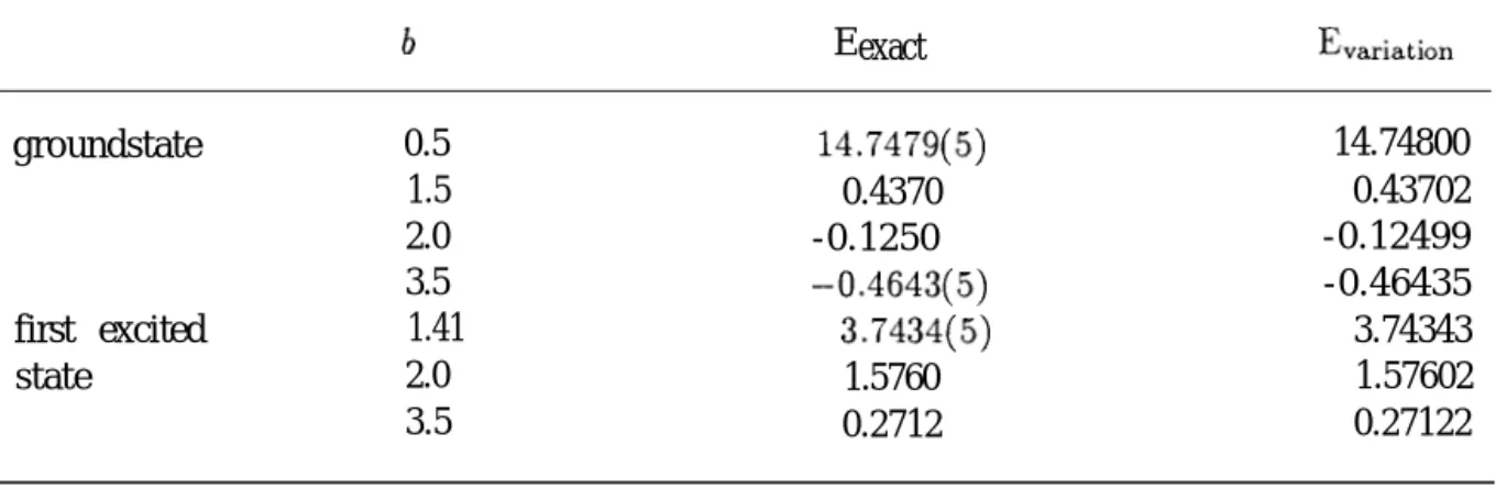
To demonstrate to what extent the numerical capability can be improved in this new variational scheme, we show our data in two examples: donor states in a spherical semiconductor quantum dot with (i) an on-center donor (ii) an off-center donor. We assume the potential on the boundary of the dot is infinite and the hydrogenic-effective-mass theory is applicable. Hydrogen basis functions with principal quantum n up to 5 are used in all of the present work. After deleting linearly dependent basis functions, the available maximum number of basis functions is 12 (for the magnetic quantum number m=O). Due to the axial symmetry, the numerical integration in 3D can be reduced to a calculation in 2D. We use a 1000 x 1000 mesh points to obtain the integration results. As we compare the results from 250 x 250,500 x 500, 1000 x 1000 and 2000 x 2000 mesh points, we found the convergence of the data is well established for mesh points over 500 x 500. In the present work, the unit of the energy is expressed in effective hartree, and the unit of the distance in effective Bohr radius. The numerical data are shown in Table I, Table II.

The data in Table I and Table II show the accuracy of our calculations is quite well. It is wanted to be pointed out that our data have higher accuracy than the original work of GB, and the improvement is especially apparent at small R and large D. This fact displays that, as we said in Sec. I, the inclusion of the basis functions not only enhances the accuracy of the data but also makes the calculation scheme have much better capability in simulating the asymmetric problems. The numerical data of the first excited state also have high accuracy, which means our new variational method is also suitable for calculating the properties of excited states if the number of basis functions is large enough. When compared with the

622 EFFECTS OF THE QUANTUM SIZE AND AN OFF-CENTER.. . VOL. 36

TABLE I. The energy levels of a hydrogenic donor atom on-center in a spherical dot. b (in effective bohrs) is the radius of the sphere and the energy is of unit effective hartree. Eexact is the exact value[ref. 81 and Evariation is the value of the present work. b Eexact Evariation groundstate 0.5 14.7479(5) 14.74800 1.5 0.4370 0.43702 2.0 -0.1250 -0.12499 3.5 -0.4643(5) -0.46435 first excited 1.41 3.7434(5) 3.74343 state 2.0 1.5760 1.57602 3.5 0.2712 0.27122

TABLE II. The ground state energy (effective hartree) of a hydrogenic donor atom placed at a distance bD off the center of a spherical dot of radius b (bD in effective bohrs). Different calculations are compared, which are denoted as (a) Gorecki and Byers Brown[ref. 61. (b) D’ramond, Goodfriend and Tsonchev[ref. 91. (c) Brownstein, N = M = 6 [ref. lo]. (d) Present work.

b bD = 0.1 bD = 0.5 bD = 1.0 source 4.0 -0.48318 -0.48105 -0.47335 -0.48318 -0.48107 -0.47344 -0.48315 -0.48102 -0.47342 -0.48318 -0.48107 -0.47343 3.0 -0.42358 -0.41373 -0.37719 -0.42358 -0.41389 -0.37841 -0.42358 -0.41392 -0.37840 -0.42358 -0.41390 -0.37840 2 . 0 -0.12286 -0.06607 0.15852 -0.12285 -0.06889 0.12752 -0.12286 -0.06889 0.12751 -0.12285 -0.06889 0.12765

VOL. 36 JONE-ZEN WANG AND TZONG-JER YANG 623

original GB method, a point to be stressed is that the trial wave function as Eq. (1.1) can not usually match all required properties if a new potential is added in the quantum system. Therefore, the original GB method is not suitable for general problems where a new potential exists. With the use of basis functions, if they are comprised of a complete set, it is straight forward to our new method to solve general quantum mechanic problems. The dominant advantages of original GB method come from two facts that the boundary condition is satisfied at every point on the boundary of the system and quantum systems with special forms can be simulated, although the accuracy may be not good for systems of low symmetry. The important meanings of the improvement in our new method are not only to diminish the drawback which GB method encounters but also to extend GB method to become a general variational tool to solve the Schrodlnger equation.

111-Z. D o n o r s t a t e s i n s p h e r i c a l a n d e l l i p s o i d a l q u a n t u m d o t s

In literature, to our knowledge, the calculations on quantum dots are restricted to simple or highly symmetric systems, like the cubic or the spherical dots. A special advantage of the GB and our method is the calculations in systems of special shapes can also be performed. In this section we discuss donor states in a semiconductor quantum dot

-0.3 ’ I

1.0 2.0 3.0 4.0

b

FIG. 1. Normalized energy levels of a on-center donor in a spherical quantum dot as a function of the dot radius

b (effective Bohr radius). The

ener-gies are normalized with respect to the sixth energy level of a electron in the same dot without a donor.

I

-

m=O

--- _m=l

-..-.

m=2

b

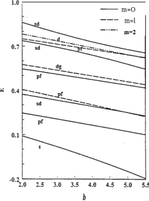
FIG. 2. Same as Fig. 1 except in a ellipsoidal dot with a = 0.56. The characters in the figure denote the symmetry of the dominant basis functions. Energy states with magnetic quantum num-ber m up to 2 are included.

624 EFFECTS OF THE QUANTUM SIZE AND AN OFF-CENTER.. VOL. 36 1.1 - m=O sd -_- m=l _..-. _m=2 -0.3 ' 1.0 '_ I 2.s 3.0 3.5 4.0 4.5 5.0 5.5 a

FIG. 3. Same as Fig. 2 except in a ellipsoidal dot with a = 2b and the x coordinate is a. 3.5 - m=O - 0 . 5

5

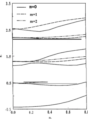
0.0 0.2 0.4 0.6 0.8 D

FIG. 4. Energy levels (effective hartree) of donor states in a spherical dot as a function of D. The donor is shifted at a distance bD from the center in the z direction. The radius of the dot

b is 3 (effective Bohr radius) and m is

taken to be 0, 1, and 2 only.

with impenetrable boundary surface, $+$t$=1. In general cases, a and b may be variable parameters. So, the contour surfaces may have special shape. In our calculations, although we use only the typical forms (i.e. the sphere and the ellipsoid), we think common features should exist in quantum systems of similar boundary surfaces. The effective-mass theory is assumed and the donor is allowed to be shifted, in the z axis, at a distance bD from the center. We consider three kinds of systems: a = b (sphere), a = 0.5b (ellipsoid) and a = 2b (ellipsoid). Energy spectra and binding energies of the ground state and the first excited state of quantum dots with different size are calculated. The number of basis functions used in the calculations is the same as that in last section and electronic states up to the sixth energy state are considered in following discussions.

In Fig. 1, we have plotted the spectrum of on-center donor states in a spherical quantum dot as a function of the dot radius b Here, for the sake of clearness, the spectrum are normalized with respect to the energy of the sixth energy state of an electron confined in a quantum dot of the same size (i.e. without donor atom). It is seen that all normalized energy levels change like linear functions of the radius b. The special point is the crossover

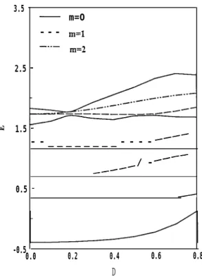
VOL. 36 JONE-ZEN WANG AND TZONG-JER YANG 625 3.5 - m=O - - - m=l -..-m=2 2.5 -H 1.5 -- -- _ _ _ _ _ _ _ _ -- -- -- -- _I--/-/ - _I-- _/0.5 --0.5 0.0 0.2 0.4 0.6 0.8 D

FIG. 5. Same as Fig. 4 except in a ellipsoidal FIG. 6. Same as Fig. 5 except in a ellipsoidal dot with with a = 0.56 and b = 5. dot with with a = 2b and a = 5.

3.0 2.5

l-

m=O

I ---

m=l

1

-.__

m=2 _{-==_C_} ___--~~-~~~'_ - _ - - - ----_ --_ --________ - 0 . 5 0.0 0.2 0.4 0.6 0.8 D .

of the 2s and 3d states. In Fig. 2 and 3, the spectra of on-center donor states in ellipsoidal quantum dots, with a = 0.5b and a = 2b respectively, are plotted as a function of b and a Each of these spectra is also normalized with respect to the energy of the sixth energy state of an electron in the same dot. As the size of a quantum dot increases the energy levels in Figs. 1, 2, and 3 decrease in quite similar ways. The major difference is the position of energy levels in the spectrum which changes due to different symmetric properties of each state. However, it is noted that the behaviors of the ground state and the first excited state in Figs. 1, 2 and 3 are similar in most respects. In Fig. 2, concerning the first pf-mixed state, the m = 1 state having higher energy than the m = 0 state is reasonable because the electron in the dot is confined more strongly in the x and y directions than in the z direction. Contrast to the Fig. 2, in Fig. 3 the dot is confined more strongly in the z direction than in the x and y directions, therefore the first pf -mixed state has the lower energy for m = 1 than for the m = 0 cases. Essentially, we can say that the roles of the first pf -mixed states with m = 0 and m = 1 are interchanged in an elongate and an oblate ellipsoids. This fact will also b,e seen in the following Figs. 5 and 6 and Figs. 8 and 9. In Figs. 4, 5 and 6, we have plotted the electronic spectrum of a quantum dot as a function of D. Because these systems have only azimuthal symmetry, the orbital angular momentum is not a good quantum number. Therefore, the basis functions are highly hybridized and the energy levels are seen to split as D increases. There seems to be no similar behaviors between the higher excited states of Figs. 4, 5 and 6. But as we have pointed out above,

626 EFFECTS OF THE QUANTUM SIZE AND AN OFF-CENTER.. . VOL. 36 - b=2 - - - b+ 0.6 0.3 ' I 0.0 0.2 0.4 0.6 0.8 FIG. 7. D

Binding energies (effective hartree) of the ground state (m = 0) and the first excited states (m = 0 and 1) in a spherical dot as a function of D. T h e donor is shifted at a distance bD form the center in the z direction. Data in two dots with radius of b = 2 and b = 3 are included. 1.8 , -b=2.5 1.4 [ \ --- b=5 0.6 1 ‘uq=l. t -\ \_\ ‘A. 0.2 ' 0.0 0.2 0.4 0.6 0.8 D

FIG. 8. Same as Fig. 7 except in ellipsoidal dots with a = 0.56 and b = 2.5 and 5.

the ground state and the first excited state in Figs. 4, 5 and 6 still have quite similar behavior.

In Figs. 7, 8 and 9, we have plotted binding energies as functions of D The binding energy is defined as Egi G EF -E; where EF and E; are respectively the ith electronic states without and with a donor in a quantum dot. It is seen in these three figures that when D increases, Egi of states with similar symmetry change in a similar way even when sizes and shapes of the dots are different. The minor differences are the magnitudes of binding energies in each dot and the D value where the binding energies of the ground state and the first excited state for m = 0 cross each other. It can be seen that the crossover goes to a larger D as the size of the dot increases. This fact can be easily explained because when the size of the dot increases, the electronic spectrum approaches to the spectrum of a free hydrogenic atom, which has no crossover between the binding energies of different energy levels. As we have mentioned above, the boundary confinement factor to the first excited states with m = 0 and m = 1 are interchanged. So, the relative magnitudes of binding energies of these two states are interchanged in Figs. 8 and 9. Finally, it should also be noted that the magnitude of the binding energy changes apparently as D increases.

VOL. 36 JONE-ZEN WANG AND TZONG- JER YANG 627 I m=O 0.6

o,r----“I___j

-0.0 0.2 0.4 0.6 0.8 D

Fig. 9. Same as Fig. 8 except in ellipsoidal dots with a = 2b and a = 2.5 and 5.

.

So, the data shown in this section tell that the properties of the ground state and the first excited state change with the size of the quantum dot in a consistent way. The shape of the quantum dot seems to have less effect on these two states. However, the higher excited states have much different behaviors for different size and shape of a quantum dot. This fact seems to be a helpful guideline in analyzing the experimental data. But, the factor that the magnitude of the binding energy changes fast when the displacement, D, of the donor atom increases should be carefully considered.

IV. Conclusions

The data shown in Sec. III-l, as compared with exact values and those from other methods, support that our new variational method is an effective and general tool for quantum systems of low and high symmetry. The basis functions in this method need not to be of special form in order to satisfying the boundary condition. This should be of particular advantage when the quantum system is of poor symmetry. The results in Sec. III-2 can be concluded as: (1) The effects from the dot size, dot shape and the position of the donor, 0, make the higher excited spectrum complicated. The further detail analysis on the higher excited spectrum is continued and will be published in the future. However, the ground state and the first excited state behave consistently in the data of our calculations. It seems to be suggested that the experimental data for these two states are suitable for theoretical analysis. (2) The binding energy changes apparently with the position of the

628 EFFECTS OF THE QUANTUM SIZE AND AN OFF-CENTER.. . VOL. 36

donor. Therefore, a proper distribution function of the donor must be established to give a convincing analysis on experimental data.

For the theoretical consideration of the method itself, our new method is a general variational tool for both of the confined and the open systems. It does not demand the $0 of Eq. (1.1) to be nodeless as in the theory of GB and the available energies and wave functions of excited states are helpful for approaching the electron-optic and electron-phonon prob-lems. In this work we consider a donor atom in a dot without other potential inside. The problem of a non-zero potential existing in the dot can also be tackled with this method. The original GB theory is not usually suitable for the problems with new potential, because if the trial function f& and the potential have different symmetry, the results would not be convincing. The fact that #u may not have the lowest energy in a system with a new potential is also an important factor to obtain inaccurate variational results. The use of basis functions in our new method can effectively resolve these difficulties if the number of basis functions is large enough. For the problems with a new potential, the only change in our method is to reformulate Eq. (2.16), w ic is a straightforward derivation. Also, due toh’ h the same reasons said above, our method can be naturally extended to open systems, i.e. the system size (the s1 in Sec. II) being infinite. Surely, without the contour function f, people can directly use basis functions to construct trial wave function and then solve the Schrodinger equation. Rather, the use of contour function f will accelerate the computa-tion, because the symmetry of trial functions is easily modified by f and less basis functions are needed in this method. The computational time grows as square of the number of the basis functions. So, when too many basis functions are needed in the open problems, our method will be a better choice. In general problems, the contour function may not have simple analytical form. For the future work, it seems to be more efficient to construct the contour function numerically.

Acknowledgments

We would like to thank Mr. C. F. Kao and Y. C. Lee for their help to in the numerical calculation. Also, we would like to thank the National Science Council of R.O.C. to support this work through Grants Nos. NSC 87-2112-M-009-034 and NSC 86-2112-M-009-022.

References

[ 1 ] A. S. Plaut, H. Bage, P. Grambow, D. Heitmann, von K. Klitzing, and K. Ploog, Phys. Rev. Lett. 67, 1642 (1991).

[ 2 ] C. Weisbuch and B. Vinter, Quantum Semiconductor Structures, (Academic Press, New York, 1991).

[ 3 ] S. Tsukamoto, Y. Nagamune, M. Nishioka, and Y. Arakawa, Appl. Phys. Lett. 63, 355 (1993).

[ 4] N. F. Johnson, J. Phys.: Condens. Matter 7, 965 (1995).

[ 5 ] J. L. Zhu, J. Wu, R. T. Fu, H. Chen, and Y. Kawazoe, Phys. Rev. B55, 1673 (1997). [ 61 3. Gorecki and B. W. Brown, J. Phys. B22, 2659 (1989).

[ 7 ] J. L. Marin, R. Rosas, and A. Uribe, Am. J. Phys. 63(5), 460 (1995). [ 8 ] J. L. Marin and S. A. Cruz, Am. J. Phys. 59(10), 931 (1991).

[ 9 ] J. J. Diamond, P. L. Goodfriend, and S. Tsonchev, J. Phys. B24, 3669 (1991). [lo] K. R. Brownstein, Phys. Rev. Lett. 71, 1427 (1993).