A FLEXIBLE PARALLEL ARCHITECTURE FOR RELAXATION LABELING ALGORITHMS

(1)

IEEE TRANSACTIONS ON SIGNAL PROCESSING, VOL. 40, NO. 5, MAY 1992 1231

A Flexible Parallel Architecture for Relaxation

Labeling Algorithms

Shaw-Yin Lin and Zen Chen

Abstract-The design of a flexible parallel architecture for both the discrete relaxation labeling (DRL) algorithm and the probabilistic relaxation labeling (PRL) algorithm is addressed. Through the analysis of parallelism in the computational models of both algorithms, the parallel execution of the algorithms on a flexible parallel architecture i s presented. Three basic types of parallel operations are performed in the architecture: simul- taneous, pipeline, and systolic. An illustrative example is used to show how the DRL algorithm can be executed on the parallel architecture. In doing so the processing element (PE) organi- zation and the combiner organization of the architecture are described. The same architecture with programmable func- tional units is shown to be able to execute the PRL algorithm, too. The performance comparisons between the proposed ar- chitecture and some other existing ones are also given.

I. INTRODUCTION

ELAXATION labeling algorithms have been applied

R

successfully to a number of applications, for instance, signal restoration, language identification, graph homomorphism, image segmentation, and scene interpre- tation [1]-[8]. One of the major issues of using this type of algorithms is that it is computationally intensive and requires typically an exponential execution time on a single processor architecture [9]. Many researchers have tried to build fast architectures [9]-[15] for executing the relaxation labeling algorithms. Uresin and Dubois [ 101, Zenios and Mulvey [7], and Kamada et al. [ l l ] proposed the multiprocessor approaches. They were faced with the difficulties in task partitioning, scheduling, and synchronization among multiprocessors. Resis and Kumar [ 121, and Derin and Won [13] used mesh connected computer (MCC) architectures to approach the relaxation problems. Their techniques have an appealing run time performance from a theoretical viewpoint, but suffer from physical re- alization problems such as data communication conges- tion and 110 routing complexities. Most of the above approaches remain in the phase of virtual software simu- lations [9]. Lately, there has been an increasing interest in implementing relaxation operations by using dedicated hardware architecture that can be built in a modular fashion, for instance, in the form of systolic arrays. Several preferential factors of the systolic approach, such as the

Manuscript received August 28, 1989; revised April 17, 1991. The authors are with the Department of Computer Science and Infor- mation Engineering, National Chiao Tung University, Hsinchu, Taiwan, 30050, Republic of China.

IEEE Log Number 9106553.

feasibility of pipelining, high degree of parallelism, and avoidance of global communication, make the arrays suitable for VLSI fabrication. Among these architectures are the works by Derin and Won [13], Gu et al. [14], Guerra

[ 151, and Bridges et al. [ 161. The underlying idea behind these methods is the application of suitable transforma- tions to the relaxation algorithms to obtain a representa- tion that can be easily mapped onto their proposed architecture. Thus, different relaxation labeling algorithms give rise to different array designs. However, the function of resultant systolic array is somewhat restricted simply because the applied architecture is too fixed to cover different applications.

In this paper, we consider the relaxation labeling algorithms in two different forms: discrete relaxation labeling (DRL) and probabilistic relaxation labeling (PRL). Both of them are executable on our proposed architecture. The arrays of the architecture use one-dimensional, one- way communication lines between adjacent PE’s and in- teract with the external environment through a single U0 port. Because of the hardware simplicity and programmability features of the PE’s, the architecture is well suited for VLSI implementation and is flexible enough to be adaptable to a number of applications. Moreover, the proposed architecture will run in a linear time for each iteration of labeling process. It is also able to check the consistency status of the DRL algorithm and the convergence condition of the PRL algorithm at the hardware level without the host involvement. On the other hand, the use of one-way flow through the arrays simplifies the circuit design and the system can be converted to self- timed arrays to avoid the clock skew problem for large labeling processes [ 181.

The paper consists of five sections. Section I1 presents the overview of the two relaxation labeling algorithms: DRL and PRL. In Section 111, parallelism in the two relaxation mathematical models is the key to our design of a flexible parallel architecture. Three basic types of parallel operations are used: simultaneous, pipeline, and systolic. The processing element organization of the systolic array and the combiner organization are then introduced. An illustrative example is used to show how the DRL algorithm is executed on the architecture. The same architecture with programmable functional units is also shown to be able to execute the PRL algorithm. Section IV cov- ers the performance comparisons between our architec-

(2)

summary.

11. OVERVIEW OF Two RELAXATION LABELING G i v e n a s e t o f N o b j e c t s U = { U l , U 2 , e . . , U N } and

a set of M labels A = { XI, A2, ,

A,

} , a relaxation labeling algorithm attempts to assign iteratively the labels to all objects such that these object-label assignments are consistent with a set of prespecified compatibility constraints (or coefficients) between the pairs of object-label assignments. We shall consider two types of algorithms: discrete relaxation labeling (DRL) and probabilistic relaxation labeling (PRL).

ALGORITHMS *

A . Discrete Relaxation Labeling (DRL)

In this case the labels are assigned to objects in an all- or-none fashion. The prespecified compatibility coefficients CC = {C,,J( A,, A,), i , j E [ l , N I ; t , p E [ l , MI}

are such that Cl.,(

A,, A,)

= 1 if the assignment of label A, to objects U, is compatible with the assignment of label A, to object U, and 0 otherwise. In the iterative relaxation labeling process for each object U,, i E [ l , NI, let L f ( A )

= [ L f ( A I ) , L f ( A,), * * , L f ( A,)] denote the vector of the label assignments given to ob‘ect U, at the kth iteration, k = 1, 2, 3 , * * , where Li(

A,)

= 1 if label A, is assigned to U, and 0 otherwise. The complete list of object-label assignments, called a labeling

zk,

is indicated by L k = {,$(A), G(A), , L h ( A ) } . Initially, each object U, is assigned to have all labels in A , i.e., L:(

A,)

= 1 f o r k = 0, i E [ l , NI and t E [ l , M I . Ob- viously, these initial assignments may not be consistent with the prespecified compatibility coefficients, so the labeling will be updated through the following formula:

N M

L:+’(A,) = Lf( A,)

*

rI

[

C,,,(A,, A,)

*

L:(Ap)] 5’1 p = l

k = 0, 1, 2, 3, *

-

* (1) where

*,

U, and

C

denote the Boolean AND, PRODUCT, and SUM operations, respectively. When there exists some finite constant K such that k 2 K , L f f l ( A,) = Lf ( A,) for all i E [ 1, N] and t E [ 1, M I , then the labeling process is said to satisfy the consistency condition and the process stops.

B. Probabilistic Relaxation Labeling (PRL)

The PRL algorithm can be thought as a generalization of the DRL algorithm. The algorithm assigns different probabilities, instead of the zero-or-one fashion, to the object-label pairs. The probabilistic labeling estimates of object Ui E U , denoted by Pi( A t ) , t E [ l , MI, are ranged in the interval [0, 13 and will be updated during each iteration. The heuristic knowledge embedded in what are termed compatibility coefficients CC = { C i , j ( A,, A,), i, j E [ l , N I ; t , p E [ l , M I } is to control the contribution that the probability of assigning label A, to object V j made

torically, C i , j ( A,, A,) is so defined that it takes a value in the range of [ - 1, 11 where - 1, 0 and 1 indicate “totally incompatible,” “independent,” and ‘‘totally compatible,” respectively. The initial labeling estimate of P:( A,), f o r k = 0, i E [ l , NI and t E [ l , M I , is estimated based on the information available on hand. The iterative updating of the labeling of object

Ui,

i E [ 1, NI, is given by

P f + ’ ( A,)

for i E [ l , N I , t E [

$(A,) =

,

MI,

and k = 0, 1 , 2 , 3 , *

.

, where

N M

The updating of these labeling estimates stops if the estimates are unchanged or nearly unchanged after a certain finite number of iterations. In this case, it is said a convergence condition is reached.

111. PARALLEL EXECUTION OF RELAXATION LABELING ALGORITHMS

A. n e DRL Algorithm

In the following we shall examine the parallelism in the computation models of both DRL and PRL algorithms. From this analysis of parallelism we shall determine three basic types of parallel operations for hardware execution of these algorithms. We shall first describe the architecture for the DRL algorithm, then point out the necessary modifications of the DRL architecture needed in order to execute the PRL algorithm.

To illustrate the idea more explicitly, let us consider a region color labeing problem [13]. Suppose that we are analyzing a picture with five regions which are to be col- ored in red, green, and blue, subject to certain compatibility constraints. The DRL formulation for this problem is given below:

I

1) A set of five regions U = { U l , U,, U,, U,, U,} where

Ui

= region

i.

The object set size is N = 5.

2) The coloring labels A = { A I , A2,

A,}

where A I is red, A2 is green, and A3 is blue. The label set size is M =

3.

3) The compatibility coefficients (or constraints) between any two region label assignments C j , j ( A,,

A,)

i , j E [ l , 51 and t , p E [ I , 31. Let us rewrite (1) as follows: For i , j E 11, 51 and t , p E [ l , 31

3

S!,j(At) = Ci,j(Ar,

*

~ ; ( x p ) (3a)

(3)

LIN AND CHEN: FLEXIBLE PARALLEL ARCHITECTURE FOR RL ALGORITHMS 1233

-4

The main module

4

The combiner module

I-+--

Fig. 1 . The organization of the proposed architecture

TABLE 1

THE LIST OF DATA S T R E A M S DURING EACH C L O C K C Y C L E FOR T H E DRL EXAMPLE: THE I N P U T DATA S T R E A M S AT T H E Y,, A N D

x,,

ENDS

Clock 0 1 2 3 4 5 6 7 8 9 l o l l . . . 25 26 27

LF+'(A,) = &A,)

*

$(A,)

All computations in (3) will be executed in parallel on a parallel architecture to be introduced below. There are totally N X M = 15 supporting evidences, i.e., Si( A,), i

= 1, 2, 3,

4,

5 and t = 1, 2, 3. They are divided into

{SI< S A

A d ,

S3(

A d ,

Sd

A d ,

Sd

A d } ,

and (SI( A3) S2( A3), S3( A3), S4( A,), S,( A3)}. These three groups are to be executed, respectively, by three linear rows of processing elements (PE's). The physical arrangement of these computations is shown in Fig. 1. All computations are done in three different ways:

1) Simultaneous computation. The computations of

$ ( A I ) ,

Ss( h ~ ) , and S f ( A 3 ) ,

i E

[ l ,

51, specified by (3b) are simultaneously executed in the three rows of PE's.

2) Pipeline computation. The computations of SI( A,),

Sz(

A t ) , S3( A,), S,( A,), and S,( A t ) , are computed in a

pipeline order in the tth row where t E [ l , 31. Also the new labeling estimates L';' I ( A,), L i f ' (A,), L i + I (A,),

Lt+'(A,),

and L : + ' ( A , ) , specified by (3c) are generated in a pipeline order in the combiner module, too.

3) Systolic computation. The Boolean product specified by (3b) for some i E [ 1, 51 is executed in a systolic manner, because it involves the input stream of labeling estimates ~ ! ( * ) , j = 1, 2 , , 5 , in (3a). The detailed description will be given later. One the other hand, since three groups:

{SIC

AI), SZ( A I L Sd AI), S4( AI), S,( AI)},

all variables SF,,( A,), C , J ( A,, A,) and L,k( A,) in (3a) are 1-b wide, we can use the logic gates with 1-b inputs to implement (3a). However, we shall pack M 1-b labels A I , A2, * *

-

, AM(M = 3) into an M-bit label vector

A

to represent all labels. So (3a) will be executed by a Boolean circuit with M-bit inputs. From now on, we use

Lf(A)

to represent the 3-b vector [L;( A,), L:( A2), L:( A?)].

Next we shall describe, in more detail, i) how the systolic computation of

Si

( A,) is done in the first row of five PE's in the main module, and ii) how the pipeline computation of L;"

(A)

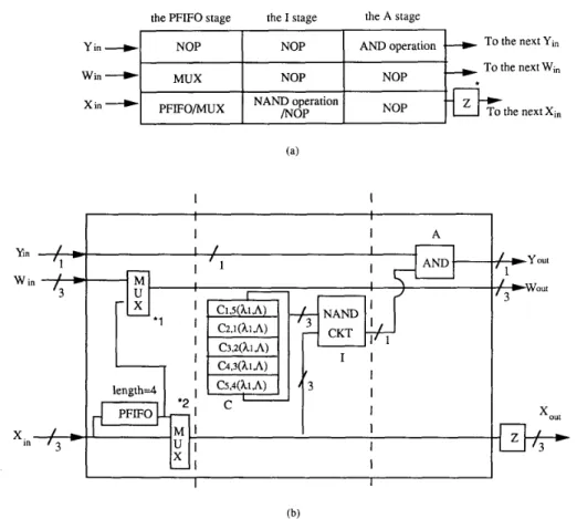
is done in the combiner module. We shall introduce the required hardware architecture, too.

First of all, the input data streams at the Y,, and X,, ends of the first PE's of all the three rows are given in Table I. These input streams will step through the PE's in each row simultaneously. The three pipeline stages of a PE, as shown in Fig. 2(a), are so designed that:

1) The first PFIFO stage is to delay the input stream at XI, end of the first PE for N - 1 =

4

clocks in order to synchronize the

Lf(A)

stream with the

SF(A)

stream generated at the output end of the last PE for computing the new labeling estimate

L;+'(A)

stream specified in (3c). The delayed Lf (A) stream is fed to the W line.

2) The

I

stage is to compute

Si,,(

A , ) of (3a) for some j E [ I , 51.

3) The A stage is to compute some partial product of S:( A,) of 3(b).

4)

The Z buffer is to adjust the data flow rate on the

X,,, line such that it is one clock behind that on the Y line. This synchronization is needed in the systolic operation for executing (3b).

(4)

AND operation ,---t

-

To the next Yi, To the next Win

Y i n L NOP NOP

-.

NOP NOP I I I I A I I I I (b)

Fig. 2. (a) The three pipeline stages of a PE. *Z is a one-clock delay buffer. (b) The hardware organization of the PE for the implementation of the DRL algorithm. *1: The multiplexer selects the input from PFIFO in the first PE of each row, and it selects the W , , input in all the subsequent PE's. *2: For the DRL mode, this multiplexer always selects the bottom input.

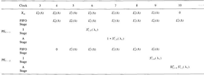
Let us see how the actual systolic operation takes place in the first row of PE's. For instance,

All the partial Boolean products of S'; ( A,) will be generated one at a PE in a fixed order from PEI

-

to PE, - 5 r

as shown above. The first partial product is S i , , ( A,) in which we need L : ( A ) . L : ( A ) arrives at the Xi, end of PE1 - during clock 4 and passes through the PFIFO stage at clock 5 . The computation of S';,5 ( A,) = E; = I C , ,

,

( A I ,

A,)

*

Lt(

A,)

is performed at the I stage by a two-level NAND circuit during clock 6. In the cycle of clock 7, the first partial product

II;=,

S f , j ( A,) is computed at the A stage of PEI - I by an AND gate. The result is output

(5)

LIN AND CHEN: FLEXIBLE PARALLEL ARCHITECTURE FOR RL ALGORITHMS 1235 TABLE I1

THE TIME-SPACE SNAPSHOTS O F PE CONTENTS IN EACH CLOCK CYCLE FOR COMPUTING T H E PARTIAL PRODUCTS OF S:( hi ) I N PE, ~ I A N D PE, ₂

Clock 3 4 5 6 7 8 9 10 I Stage A Stage PE,

-,

TABLE 111

THE LIST OF DATA STREAMS DURING EACH CLOCK CYCLE FOR T H E DRL EXAMPLE: THE GENERATFD S t ( XI ). S:( A?), S:( A,), AT T H E Y,,,, ENDS OF T H R E E LINEAR ARRAYS

Clock 19 20 21 22 23 24 25 . . . 44 45 46

Table 11. Similarly, St,,(

X I )

= c1.4(

X I ,

A,)

*

L:( X p ) is computed at the I stage of PE, - during clock

9 . The partial product

n;,,

St,,(

X I )

is then generated at the A stage during clock 10. The growth of the partial product continues to take place at PEI - 3, PE,

-,,

and PE, - S . And the final result of S'; ( X I ) =

IIl=

I Si,, ( X I ) is

obtained during clock 19, as indicated in Table 111.

Si

(

A,)

and Si (

A,)

are simultaneously generated in the second and third rows, when S!(

X I )

is generated in the first row. The subsequent supporting evidences Sf ( A,) for

i = 2 , 3 ,

- -

, are generated in the same way during the clock cycles given in Table 111.

The correct values of supporting evidence generated above in each row rely on the proper pairing between the compatibility coefficients and the labeling estimates, as given in (3a). The compatibility coefficients are arranged in a circular shift register in the five PE's of the first row and are ordered according to the required timing relations needed to compute SI(

XI),

S,( A,), S3( A,), S4( A,), and S5( A,) in the first row of Fig. 3.

The compatibility coefficient arrangements in the PE's of other rows in Fig. 3 can be obtained by simply changing

X I

to

X2

for the second row, and changing

X I

to

A3

for the third row.

Next, consider (3c) for computing the new labeling estimates. The generated new labeling estimate stream at the R,,, end is shown in Table IV. Let us see how L:+

'

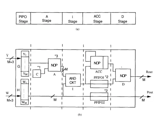
(A)

is generated during clock 24 in the combiner module. The combiner organiztion consists of five pipeline stages, as shown in Fig. 4. It takes five clocks to generate a new labeling estimate. At clock 20, the generated S';(

XI),

S:( A,), and S i ( A3), are output as S!(A), by a parallel- in-and-parallel-output (PIPO) G registers at the PIPO stage. The labeling estimate L i ( A ) passes through the PIPO stage via

H

registers at clock 20, too. At clock 21, $(A) passes through the A stage without any operation. At clock 22, the Boolean ANDing operation of L ! ( A )

*

S! (A) = L i t ' (A) is performed at the I stage. At clocks 23 and 24, the result

L$+'(A)

steps through the last two stages without any operations. Thus at the end of clock 24, L!' I (A) appears at the R,,, end. The reason for using

the NOP (no operation) mode of A , ACC,

D

stages in the combiner is to allow this same combiner structure to be used in a programmable mode to handle the probabilistic relaxation labeling (PRL) algorithm. The other new labeling estimates are generated similarly in a pipeline order, as shown in Table IV. At clock 25 the new stream of

L!+~(A),

i = 1, 2 , , and the old stream of Lf;(A), i = l , 2 ; * * , obtained at the R,,, and Po,, ends are com- pared at the hardware level to determine the consistency condition. At clock 26 the new stream of

Lf"

(A),

i

= 1, 2,

This completes our description of the parallel execution (or mapping) of the given DRL algorithm on our parallel

.

(6)

PIP0 Stage

A I ACC D

Stage Stage Stage Stage

TOP

(at clock 6) (at clock 9) TOP (at clock 12) TOP (at dock TOP 15) (at clock TOP 18)

The compatibility coefficient arrangements in the PE's of the first row.

Fig. 3

TABLE 1V

THE L I S T O F D A T A STREAMS D U R I N G E A C H CLOCK CYCLE FOR T H E D R L E X A M P L E : T H E NEW A N D OLD L A B E L I N G E S T I M A I E S T R E A M S 4T I?,,,,, ANI) P,,,, ENDS

Y ,

M = 3

5

M = 3 Rout

/M-

Pout

Fig. 4 . (a) The five pipeline stages of the combiner module. (b) The hardware organization of the combiner module. * I : The constant buffer is not used in the D R L mode. *2: Both PFlFOl and PFIF02 are short circuited in the D R L mode. *3: The A , ACC, and D stages are set to the no operation mode; the input data pass through intact.

(7)

LIN A N D CHEN: FLEXIBLE PARALLEL ARCHITECTURE FOR RL ALGORITHMS PIS0 Y

- .

-

Accumulator

-

16 Adder L r ACC

-

‘

16

-

Divider

-

PFIFOl A 16 Multiplier C PIS0

w

- .

PFIF02 1237 1 WRout

’

16 1 ,Pout ‘8 Yin Win A / L / ‘16 1

’

16 Adder / M

I

To the next Y;,

k

6-

To thenextW,

To the next X,

G

architecture. Next, we shall modify this parallel architecture so that it can execute the PRL algorithm, too.

B. The PRL Algorithm

lows:

Let us rewrite a 5-object, 3-label PRL algorithm as fol-

5

Sf;(A,) = j =

c

I S;,j(A,)

for i, j E [ l , 51 and

In (4a) S:,,(X,), Cl,,(Af, A,), and P,”( A,) are real numbers instead of 1-b-wide binary numbers as in the DRL case. A real number here is represented by 8 b. We shall not pack M 8-b labeling estimates P i ( A I ) , P,”( A2), P i (A,) into one 3 x 8-bit datum as before, because it is not practical to use such a 24-b-wide data at the input line. Instead, we will use the 8-b-wide data to represent our input stream. We shall implement S:,, ( A , ) in (4a) by a linear systolic array of three PE’s. On the other hand, Sf ( A , ) in (4b) is again computed through a systolic operation as in the DRL case. In total, we need 3 x 5 = 15 PE’s in order to obtain the final result of S:( A,) for each i E [ l , 51.

The necessary modifications of the previous DRL architecture for executing the PRL algorithm are as follows. The architecture modifications are shown in Fig. 5.

1) The I stage is configured as a multiplier. 2) The A stage is configured as an adder.

3) The number of PE’s in each row is extended to 15. 4) The lengths of the PFIFO buffer in the first PE’s of the three rows are 14, 13, and 12, respectively, where 14

(8)

STREAMS AT T H E k',, AND

x,.

ENDS

Clock 0 1 2 3 . . . 14 15 16

TABLE VI

THE LIST O F DATA STREAMS DURING EACH CLOCK CYCLE FOR T H E PRL EXAMPLE: THE GENERATED s f ( A , ) ,

sl( A>), sr( A,) A T THE Yo,, ENDS OF THREE LINEAR ARRAYS

. . .

71

. . .

Clock 59 60 61 62

TABLE VI1

THE LIST OF DATA STREAMS DURING EACH CLOCK CYCLE FOR THE PRL EXAMPLE: THE NEW AND OLD LABELING ESTIMATE STREAMS AT R,,, A N D P,,,, ENDS

TABLE VI11

THE DIFFERENT MODES OF THE FUNCTIONAL UNITS FOR THE EXECUTION O F T H E DRL A N D PRL ALGORITHMS

PE The Combiner Module

I A G H A I ACC D

DRL NANDckt AND P I P 0 NOP AND NOP NOP

PRL Multiplier Adder PIS0 Adder Multiplier Accumulator Divider

The computation of a new labeling estimate P f + I (A,)

according to (4c) using the combiner is more complicated than before. The modifications include

1) The first pipeline stage is changed to parallel-in-and- 2) The constant buffer C is set to 1 .O to get the term of 3) The A stage is configured as an adder.

4) The I stage is configured as a multiplier.

5) The ACC stage is configured as an accumulator with 6) The lengths of PFIFOI and PFIF02 are set to

M

= 7) The D stage is configured as a divider.

Tables V-VI1 show the data streams at the clock steps for the generation of new estimates P';+l

( A l ) ,

Pt" ( A2),

. . .

.

Let us take a look at a snapshot of clock steps for where 59 = 3 X N x M

+

N x M - 1 , the result of

SB ( A , ) is available at Yo,, end and the P t ( A,) is available at WO,, end. During the next four clock cycles, the terms [ l

+

Si ( A , ) ] , [ l

+

S: (A,)] x P ! ( A , ) and the partial serial-out (PISO) registers.

1

+

$(A,).

a buffer length of M = 3. 3 .

p k f l I ( A , ) generated in the combiner. During clock 59,

sum of 0 and [l

+

S'; (A,)] x P t ( A , ) are obtained with adder, multiplier, and accumulator units. Similarly, in the clock cycles 62, 63, and 64, the terms [ 1

+

S'; ( h2)], [ 1

+

S t ( A2)] x P'; ( A2) and partial sum of [ 1

+

S'; ( A,)] X P';

(A,)

and [ l

+

S'; ( A2)] x P'; ( A2) are obtained, and then the

E;

= [ 1

+

S :

(A,,)]

X P : (A,) is obtained in clock 65. Finally, the new labeling estimate P ; + l ( A,) is produced by the divider and is output at the R,,, end in clock 66. The above process operates in a pipeline fashion, so the succeeding new estimates of P ' ; + l ( A2), P f + I ( h3),

P;+'

( A l ) , *

.

* will be produced consecutively on R,,, line at the rate of one per clock cycle. Totally, it takes 80 clock cycles to finish one iteration of the PRL agorithm.

C. The General Parallel Architecture f o r DRL and PRL Algorithms

From above, we can see a common parallel architecture can be used for executing DRL and PRL algorithms. The differences in the PE and combiner hardware organizations for these two cases can be settled by using programmable units in the organizations. The different modes of these functional units for the DRL and PRL cases are shown in Table VIII.

(9)

LIN AND CHEN: FLEXIBLE PARALLEL ARCHITECTURE FOR RL ALGORITHMS I239

TABLE IX

COMPARISONS OF PROPOSED ARCHITECTURE WITH Two OTHER ARCHITECTURES FOR T H E DRL ALGORITHMS Item of Architecture by Architecture by Our No. Comparison Gu et al. Resis et al. Architecture

1) Type of 2) Time complexity 3) Space complexity 4) I/O bandwidth in bits 5 ) Configurability 6 ) Adaptibility to architecture per iteration varying problem sizes checking 7) Consistency 2-D, 2-Wt systolic array O W x M ) t O(N x M ) O(M x M ) No limited Yes 2-D mesh connected computer O(N X M 2 ) OWz) O(N x M ) No No No 1-D, 1-W systolic array O(N x M ) O W ) Yes Yes Yes

t2-D, 2-W = two-dimensional, two-way; M = the number of labels; N = the number of objects

TABLE X

COMPARISONS OF PROPOSED ARCHITECTURE WITH Two OTHER ARCHITECTURES FOR THE PRL ALGORITHMS

No Item of Comparison Type of architecture Time complexity Space complexity I / O channel number Configurability Adaptibility to varying problem sizes status checking Convergence Architecture by Kamada et al. Architecture by Our Guerra et al. Architecture Round robin O(N x M ) t O W ) multiprocessor No difficult N o 1-D, 1-Wt systolic array O ( N 2 x M j O(N x M ) O(M 1 No Yes No 1-D, 1-W systolic array O(N x M j O(N x Mz) 1 Yes Yes Yes ~ ~~

t l - D , I-W = one-dimensional, one-way; M = the number of labels; N = the number of objects.

IV. PERFORMANCE EVALUATION

To evaluate the proposed architecture, we shall consider several evaluation factors including the time complexity, space utilization, and input channel bandwidth. The comparisons of our architecture with other relevant architectures for both DRL and PRL cases are shown in Tables IX and X, respectively.

A . The DRL Algorithm

Table IX summarizes the differences between our architecture and those by Gu et al. [14] and Resis and Ku- mar [ 121 for the execution of the DRL algorithm. Assum- ing the clock cycle time is T , the time complexity per iteration of our architecture is estimated as follows:

1) The time to produce the first new labeling estimate. It consists of two parts: a) ( N - 1) T which is the time required to wait for the arrival of L i ( A ) in order to compute the first partial result of a supporting evidence, and b) (3 X N

+

5 ) T which is the time to get through both the main module and the combiner module.

2) The time for computing the subsequent labeling estimates. There are N - 1 subsequent labeling estimates to be generated at the rate of one per clock cycle, so it takes ( N - 1) T to complete.

As a result, the time complexity for a single iteration

is O ( N ) . This indicates that the computation time depends only on the number of objects N , not on the size of classes M , while the other two architectures require O ( N X M ) and O ( N X M ~ ) , respectively.

Table IX also lists several advantageous features of our architecture, such as the communication with the external environment through only one single I/O port, the simplicity of the architecture using one-dimensional, one-way systolic arrays and, the programmability of the functional units.

B. The PRL Algorithm

Table X summarizes the differences between our architecture and those by Kamada et al. [l l ] and Guerra [15] for executing the PRL algorithm. The time complexity per iteration is estimated as follows, assuming T is the clock cycle time:

1) The time to produce the first new labeling estimate. It consists of two parts: a) ( N X M - 1 ) T which is the time required to wait for the arrival of p i (

A,)

in order to compute the first partial result of a supporting evidence, and b) ( 3 x N x M

+

M

+

4) T which is the time to get through the main module and the combiner module.

2) The time for computing the subsequent labeling estimates. There are N X M - 1 subsequent new labeling

(10)

cycle, so it takes ( N x

M -

1) T to finish.

Therefore, the total time complexity for a single iteration is O(N x

M).

Although it is of the same order as the multiprocessor architecture proposed by Kamada et al., yet the multiprocessor system takes a much longer clock cycle time than ours due to its complicated task scheduling and synchronization. On the other hand, ours is su- perior to the architecture proposed by Guerra as far as the time complexity is concerned. However, our architecture needs more PE’s than the other two architectures. Never- theless, our PE circuit is simpler and can be implemented in a high density VLSI chip. Furthermore, the convergence condition can be checked in our architecture at the hardware level without the host involvement, while the other two systems cannot do so.

V . SUMMARY

We have presented a flexible parallel architecture for executing the DRL and PRL algorithms. The architecture is designed based on the analysis of the parallelism in the mathematical models of the algorithms. We preload the compatibility coefficients into the PE’s so that only the stream of labeling estimates need to step through the PE’s. The one-dimensional, one-way layout of systolic arrays is suitable for VLSI fabrication. The performance evalu- ations listed in Tables IX and X show that the proposed architecture is generally better than the existent architectures.

In order to verify the design of the proposed systolic array and the combiner module, a simulation software package called DAISY system [ 191 has been used to check the specification. We have finished the logic simulation to check the timing sequence for the architecture operation and the signal simulation to verify the intermediate processing results. The experiments show that the proposed architecture is working properly. Future work in- cludes the development of the VLSI customer chip and proper architecture modifications to cover a wide spec- trum of related algorithms.

REFERENCES

[ I ] D. H. Ballard and C. M. Brown, Compuier Vision. Englewood Cliffs, NJ: Prentice-Hall, 1982.

121 A. Bundy, “Catalogue of artificial intelligence tools,” in Symbolic Compuiaiion Ariijicial Intelligence, L. B o k , A. Bundy, P. Hayes,

and J. Siekmann, Eds.

[3] B. Nudel, “Consistent-labeling problems and their algorithms: Ex- pected-complexities and theory-based heuristics,” Artijicial Intell.,

vol. 21, pp. 135-178, 1983.

[4] A. Goshtasby and R. W. Ehrich, “Contextual word recognition using probabilistic relaxation labeling,” Part. Recog., vol. 21, no. 5, pp. 455-463, 1988.

151 F. A. Mota and F. R. D. Velasco, “A method for the analysis of ambiguous segmentation of images,” IEEE Trans. Part. Anal. Ma- chine Iniell., vol. PAMI-8, pp. 755-760, Nov. 1986.

161 J. F. Boyce, J. Feng, and E. R. Haddow, “Relaxation labeling and the entropy of neighborhood information,” Pairern Recog. Leit. , vol.

6, pp. 225-234, Sept. 1987.

[7] S . A. Zenois and J. M. Mulvey, “A distributed algorithm for convex

network optimization problems,” Parallel Compuiing, vol. 6, pp. 45-

56, 1988.

[8] R. A. Hummel and S . W. Zucker, “On the foundations of relaxation

labeling processes,” IEEE Trans. Parr. Anal. Machine Intell. , vol. PAMI-5, pp. 267-287, May 1983.

Berlin: Springer, 1984.

strategies for the consistent labeling problem,’’ IEEE Trans. Com- put., vol. C-34, pp. 973-980, Nov. 1985.

[ I O ] A. Uresin and M. Dubois, “Sufficient conditions for the convergence of asynchronous iteration,” Parallel Compuiing, vol. 10, pp. 83-92, 1989.

[ I I ] M. Kamada, K. Toraichi, R. Mori, K. Yamamoto, and H. Yamada, “A parallel architecture for relaxation operations,” Putt. Recog., vol.

21, pp. 175-181, 1988.

[12] D. Resis and V. K. P. Kumar, “Parallel processing of the labeling problem,’’ in Proc. IEEE Comput. Soc. Workshop Comput. Archi- tecture Pati. Anal. Image Database Manag., 1985, pp. 381-385.

[I31 H. Derin and C . S . Won, “A parallel image segmentation algorithm

using relaxation with varying neighborhoods and its mapping to arrays processors,” Cornput. Vision Graph. , Image Processing, vol.

40, pp. 54-78, 1987.

[14] J. Gu, W. Wang, and T . C . Henderson, “A parallel architecture for discrete relaxation algorithm,” IEEE Trans. Pati. Anal. Machine In-

tell., vol PAMI-9, pp. 816-830, Nov. 1987.

[15] C. Guerra, “Systolic algorithm for local operations on images,” IEEE

Trans. Comput., vol. C-35, pp. 73-77, Jan. 1986.

[I61 G. E. Bridges, W . Pries, R. D. McLeod, M. Yunik, P. G. Gulak, and H. C. Card, “Dual systolic architecture for VLSI digital signal processing systems,” IEEE Trans. Cornput., vol. C-35, pp. 916-920, Oct. 1986.

(171 A. Rosenfeld, R. A. Hummel, and S . W . Zucker, “Scene labeling

by relaxation operations,” IEEE Trans. S y s i . , Man, Cybern., vol.

SMC-6, pp. 420-433, June 1976.

[I81 0. H. Ibarra and H . A. Palis, “VLSI algorithms for solving recur- rence equations and applications,” IEEE Trans. Acoust., Speech, Signal Processing, vol. ASSP-35, pp. 1046-1052, July 1987.

[ 191 Advanced Simulation, Daisy System Corp., Student’s Workbook,

1986.

L

Shaw-Yin Lin was born in Taiwan, Republic of

China, in 1953. He received the B.Sc., M.Sc., and Ph.D. degrees from National Chiao Tung University, Republic of China, in 1976, 1980, and 1990, respectively, all in computer science and information engineering.

He joined Honeywell Company in Taiwan in 1979. He became a Technical Manager there in 1981, involved in the design and implementation of the advanced industrial control systems (1981- 1986) and the intelligent enterprise management systems (1986-1990). From 1982 to 1984 he was also a part-time lecturer in the Department of Electronics Engineering and Technology at National Taiwan Institute of Technology. In 1991, he joined, as the Vice President, K&C Technologies, Inc., Taiwan. His research interests include parallel algorithm and architecture design, computer vision, pattern recognition, and artificial intelligence.

Dr. Lin received in 1976 the Phi-Tau-Phi Award for best student in his class. He also received the Outstanding Manager Award from Honeywell in 1986. He is a member of ASHARE, the Chinese Image Processing and Pattern Recognition Society, and the Chinese Engineering Society.

Zen Chen received the B.Sc. degree from Na-

tional Taiwan University, Taiwan, Republic of China, in 1967, the M.Sc. degree from Duke Uni- versity, Durham, NC, in 1970, and the Ph.D. degree from Purdue University, West Lafayette, IN, in 1973, all in electrical engineering.

From 1973 to 1974 he worked for Burroughs Corporation, Detroit, MI, where he was engaged in the development of document recognition systems. Since 1974 he has taught at the Institute of Computer Science and Information Engineering, National Chiao Tung University, Taiwan. He was the Director of the In- stitute from 1975 to 1981, and from 1989 to 1991. He spent the academic year 1981 to 1982 at Lawrence Berkeley Laboratory, University of Cali- fornia, Berkeley, as a Visiting Scientist and also spent six months on sab- batical (starting from August 1989) at the Center for Automation Research, University of Maryland at College Park, as a Visiting Professor. His areas of interest include computer vision, pattern recognition, expert systems, parallel algorithm and architecture, computer graphics, and CAD/CAM systems.