Effective Utility Mining with the Measure of
Average Utility
*
Tzung-Pei Hong
1, 2, Cho-Han Lee
3and Shyue-Liang Wang
41
Department of Computer Science and Information Engineering
3
Department of Electrical Engineering
4
Department of Information Management
National University of Kaohsiung, Kaohsiung, 811, Taiwan 2Department of Computer Science and Engineering National Sun Yat-sen University, Kaohsiung, 804, Taiwan tphong@nuk.edu.tw, prescott2005@hotmail.com, slwang@nuk.edu.tw
ABSTRACT
Frequent-itemset mining only considers the frequency of occurrence of the items but does not reflect any other factors, such as price or profit. Utility mining is an extension of frequent-itemset mining, considering cost, profit or other measures from user preference. Traditionally, the utility of an itemset is the summation of the utilities of the itemset in all the transactions regardless of its length. The average utility measure is thus adopted in this paper to reveal a better utility effect of combining several items than the original utility measure. It is defined as the total utility of an itemset divided by its number of items within it. The average-utility itemsets, as well as the original utility itemsets, doesn’t have the “downward-closure” property. A mining algorithm is then proposed to efficiently find the high average-utility itemsets. It uses the summation of the maximal utility among the items in each transaction with the target itemset as the upper bound to overestimate the actual average utilities of the itemset and processes it in two phases. As expected, the mined high average-utility itemsets in the proposed way will be fewer than the high utility itemset under the same threshold. The proposed approach can thus be executed under a larger threshold than the original, thus with a more significant and relevant criterion. Experiments results also show the performance of the proposed algorithm.
Keywords: utility mining, average utility, two-phase mining, downward closure.
*This is a modified and expanded version of the paper “Mining high average-utility itemsets”, presented at the 2009 IEEE International Conference on Systems, Man, and Cybernetics, 2009, USA.
1.
Introduction
Mining frequent itemsets from a transaction database is a fundamental task for knowledge discovery such as association rules [2], sequential patterns [4, 5, 12] and
classification [14, 24]. Its goal is to identify the itemsets with their appearing
frequencies above a certain threshold. Numerous methods were proposed in the past
to discover frequent itemsets, such as level-wise algorithms [2, 8-10, 23] and
pattern-growth methods [1, 11, 13, 16, 17]. These approaches treated all the items in a
database as binary variables, only considering whether an item is bought in a
transaction or not. In this case, frequent itemsets just reveal the frequency of
occurrence of the itemsets, but do not reflect any other factors, such as price or profit. In some situations, frequent itemsets may only contribute a small portion to the overall profit, while non-frequent ones may contribute a large portion to the profit
[22]. For example, sale of diamonds may occur less frequently than that of clothing in
a department store, but the former gives a much higher profit per unit sold than the
latter. Only Frequency is thus not sufficient to identify the items which are highly
profitable or have other potential effects.
Utility mining [25] is thus proposed to partially solve the above problem. It may be thought of as an extension of frequent-itemset mining with the sold quantities and
itemset is said useful to a user if it satisfies the utility constraint; that is, the utility of
the itemset must be larger than a threshold defined by the user. In practice, the utility
value of an itemset can be measured in terms of cost, profit or other measures from
user preference. For example, someone may be interested in finding the itemsets with
good profits and another may focus on the itemsets with low pollution while
manufacturing.
In utility mining, local transaction utility and external utility are used to measure the utility of an item. The local transaction utility of an item is directly obtained from
the information stored in the transaction dataset, like the quantity of the item sold in
the transaction. The external utility of an item is given by the user, like a profit.
External utility often reflects user preference and can be represented by a utility table
or a utility function. By combining a transaction dataset and a utility table together,
the discovered itemset will better match a user’s expectations than by only
considering the transaction dataset itself.
In frequent-itemset mining, the Apriori-like strategy [3] is often adopted to search for frequent itemsets level by level. The basic principle of the Apriori-like
strategy is the “downward closure” property (anti-monotone property). That is, any
superset of a non-frequent itemset is also non-frequent. This anti-monotone property
early. The “downward closure” principle cannot, however, be directly applied to
discover high utility itemsets. Without the “downward closure” property, the number
of candidate itemsets generated at each level is close to all the combinations of all the
items. The computation time for handling this thus becomes intolerable. Liu et al. then
presented a two-phase algorithm for fast discovering all high utility itemsets [21, 22]. In this paper, we proposed a new idea to evaluate the utilities of itemsets. Traditionally, the utility of an itemset is the summation of the utilities of the itemset in
all the transactions regardless of its length. Thus, the utility of an itemset in a
transaction will increase along with the increase of its length. That is, longer itemsets
in a transaction result in higher utility values. Thus, using the same minimum
threshold to judge itemsets with different lengths is not fair. In order to alleviate the
effect of the length of itemsets and identify really good utility itemsets, the average
utility measure is adopted in this paper to reveal a better utility effect of combining
several items than the original utility measure. It is defined as the total utility of an
itemset divided by its number of items within it. The average utility of an itemset is
then compared with a threshold to decide whether it is a high average-utility itemset.
An algorithm is also proposed to find all the high average-utility itemsets.
Like two-phase mining for high utility itemsets, the proposed mining algorithm for high average-utility itemsets uses average-utility upper bounds to overestimate the
actual average utilities of itemsets for satisfying the downward closure property. The
average-utility upper bound of an itemset is designed here as the summation of the
maximal utility among the items in each transaction including the itemset. Only the
combinations of the itemsets which have their average-utility upper bounds beyond
the user-defined threshold are added into the candidate set in a level-wise way. The
downward closure property can thus be maintained in this way. That is, any subset of
an itemset with high average-utility bound must also be of high average utility.
Therefore, the size of the candidate set is substantially reduced during the level-wise
search. Only one database scan is needed to filter out the promising candidates. After
that, the second database scan is performed to find the actual average utility of each
candidate and decide whether it is desired. Finally, the performance of the proposed
mining algorithm is verified by both a synthetic and a real database. The rest of this
paper is organized as follows.
Some related utility mining algorithms are reviewed in Section 2. The definition and the meaning of the high average-utility itemsets are given in Section 3. The
proposed mining algorithm for high average-utility itemsets is described in Section 4.
An example to illustrate the proposed algorithm is shown in Section 5. The
experimental results are presented in Section 6. Conclusion and discussion are given
2.
Review of Related Mining Algorithms
Agrawal and Srikant proposed the Apriori algorithm [3] to mine association rules
from a set of transactions. It is well known and processes the data in a level-wise way.
In each pass, Apriori employs the downward-closure (anti-monotone) property to
prune impossible candidates, thus improving the efficiency of identifying frequent
itemsets. This property states that each subset of a frequent itemset must be frequent
and each superset of an infrequent itemset must be infrequent. With the property in
mining, the number of itemsets to be checked can decrease remarkably. Many other
algorithms based on the property have then been proposed to discover frequent
itemsets rapidly [9, 15, 23, 27].
In traditional association-rule mining, a minimum support is set as the threshold to decide which itemsets are relevant. The support of an itemset has to be larger than the
minimum support in order to be frequent. It does not, however, consider the quantities
sold in transactions and the profit of each item sold, which are important to some
applications as well. Yao et al. thus proposed the utility model to measure how “useful”
an itemset is by considering both the quantities and the profits of items [25]. Note that
in real applications, the sale quantities and the profits of items in transactions usually vary.
The concept of utility is thus proposed to mine relevant itemsets according to the above
multiplied by its profit. The utility of an itemset in a transaction is thus the sum of the
utilities of all the items in the transaction. If the sum of the utilities of an itemset in all the
transactions is larger than a predefined utility threshold, then the itemset is called a high
utility itemset. The goal of utility mining is thus to identify all the itemsets whose
utility values fall above the threshold defined by users.
In utility mining, the downward-closure property no long exists since the utility
of an itemset will grow monotonically and the frequency of an itemset will reduce
monotonically along with the number of items in an itemset. The two different
monotonic properties make the downward-closure property invalid in utility mining. In the past, Barber and Hamilton proposed the approaches of Zero pruning (ZP) and Zero subset pruning (ZSP) to exhaustively search for all high utility itemsets in
the database [6, 7]. They generated all the itemsets as candidates except the ones with
their local measure values (utilities) are exactly zero. Although ZP and ZSP can
discover all high utility itemsets in a database, their computation costs are, however,
very high.
Li et al. then proposed the FSM, the ShFSM and the DCG methods [18-20] to discover all high utility itemsets by taking advantage of the level-closure property.
These methods relied on the critical function of each candidate to remove useless
Besides, Yao proposed a framework for mining high utility itemsets based on mathematical properties of utility constraints. Two pruning strategies based on utility
upper bounds and expected utility upper bounds respectively were adopted to reduce
the search space. These pruning strategies were then incorporated into the mining
approach Umining and its heuristic successor, Umining_H [26].
Liu et al. then presented a two-phase algorithm for fast discovering all high utility itemsets [22]. It had two phases. In the first phase, the transaction utility was
used as the effective upper bound of each candidate itemset in the transaction such
that the “transaction-weighted downward closure property” could be kept in the
search space to decrease the number of candidate itemsets. In the second phase, an
additional database scan was performed to find out the real utility values of the
remaining candidates and identifies the high utility itemsets. Thus, one solution of
speeding up utility mining is to reduce the size of candidates in order to decrease the
time to scan a database.
3.
Mining High Average-Utility Itemsets
In this paper, we would like to find high average-utility itemsets instead of
traditional high utility itemsets. It is reasonable and can effective reduce the size of
Traditionally, the utility of an itemset is the summation of the utilities of the itemset in all the transactions regardless of its length. Thus, the utility of an itemset in
a transaction will increase along with the increase of its length. That is, longer
itemsets in a transaction result in higher utility values. For example, assume a
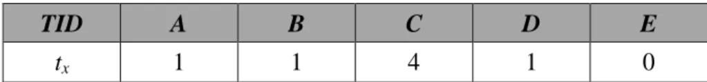
transaction is given as shown in Table 1. There are five items in the transaction,
respectively denoted A to E. The value attached to each item is the quantity sold in the
transaction.
Table 1: A transaction as the example.
TID A B C D E
tx 1 1 4 1 0
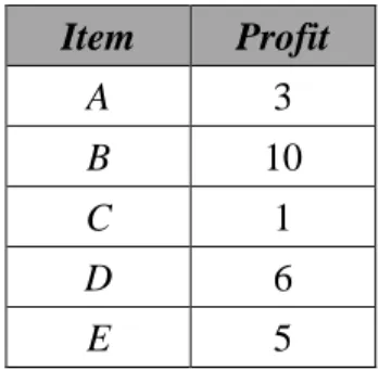
Assume the predefined profit of each item is defined in Table 2. The utility of the
1-itemset {A} in the transaction is thus calculated as 1*3, which is 3, according to the
above two tables. The utility of the 2-itemset {AB} in the transaction is calculated as
1*3+1*10, which is 13. Similarly, the utility of the 3-itemset {ABC} is calculated as
1*3+1*10+4*1, which is 17. Accordingly, the utility of the 3-itemset {ABC} is larger
than the 2-itemset {AB}, which is further larger than the 1-itemset {A}. Longer
itemsets result in higher utility values. This property is very obvious since longer
itemsets will include some more items than their proper subsets. This effect will
Table 2: The predefined profit values of the items. Item Profit A 3 B 10 C 1 D 6 E 5
Let’s give another example to show our idea. Assume there are five transactions
and only two items, A and B, in the data set shown in Table 3. Assume the sale
quantities of both the items each time are equal if they are purchased and the profits of
the two items are also the same as well. Thus, the utility values of both the items are
the same in a transaction if they are purchased. Let the utility value of a purchased
item in a transaction as X.
Table 3: The utility values of items A and B in the transactions
A B T1 X 0 T2 0 X T3 0 X T4 X X T5 X X
For the first transaction in Table 3, item A is purchased and its utility is thus X. B
is 3X. The support of B is 0.8 and the utility is 4X. However, the support of the
2-itemset AB is 0.4, but the utility of AB is 4X, which doesn’t decrease along with its
lower support value. Besides, the utility (4X) of selling A and B together in the case
does not mean better than the total utility (7X) of individually selling A and selling B.
It is because the length of the itemset {AB} is 2, which is not considered when the
utility of the itemset is calculated. The average utility measure is thus adopted in this
paper to reveal a better utility effect of combining several items than the original
utility measure. It is defined as the total utility of an itemset divided by its number of
items within it. In this example, the utility of AB is divided by 2, which is equal to 2X.
The average utility of an itemset is then compared with a threshold to decide whether
it is a high average-utility itemset. As expected, the mined itemsets in the proposed
way will be fewer than those in the original way under the same threshold. Our
proposed approach can thus be executed under a larger threshold than the original,
thus with a more significant and relevant criterion. The approach for mining useful
itemsets under the proposed criterion is stated below.
4.
The Proposed Algorithm for Mining High Average-utility Itemsets
In the proposed algorithm, the anti-monotone property is used to decrease the
algorithm. In phase 1, the average-utility upper bound is used to overestimate the
itemsets. The average-utility upper bound is an overestimated utility value instead of
actual utility value. The average-utility upper bound can ensure the anti-monotone
property. Thus, each subset of an itemset with high average-utility upper bound must
be high; each superset of an itemset with low average-utility upper bound must be low.
It can thus prune many low average-utility upper bound itemsets level by level and
decrease the time to scan a database. In phase 2, we just need to scan the database
once to check the result of phase 1 is actually high or not.
The proposed algorithm first finds all the candidate average-utility 1-itemsets C1.
The 1-itemsets whose average-utility upper bound larger than or equal to minimum
average-utility threshold are put in the set of candidate average-utility 1-itemset C1.
Candidate average-utility 2-itemsets C2 are formed from C1. The proposed algorithm
then checks all the candidate average-utility 2-itemsets C2 by comparing the
average-utility upper bound with the minimum average-utility threshold. The itemsets
which do not exceed the minimum average-utility threshold are removed from the
candidate 2-itemsets. The same procedure is repeated until all the itemsets have been
found. Then we calculate the actual average-utility value of each candidate
average-utility itemset. If the itemset is larger than or equal to the minimum
details of the proposed mining algorithm are described below.
Two-Phase algorithms for mining high average-utility itemsets
INPUT:
1. A set of m items I = {i1, i2, …, ij, …, im}, each ij with a profit value pj, j = 1
to m;
2. A transaction database D = {T1, T2, …, Tn}, in which each transaction
includes a subset of items with quantities;
3. The minimum average-utility threshold
λ
. OUTPUT: A set of high average-utility itemsets.STEP 1: Calculate the utility value ujk of each item ij in each transaction Tk as ujk =
qjk*pj, where qjk is the quantity of ij in Tk for j = 1 to m and k = 1 to n.
STEP 2: Find the maximal utility value muk in each transaction Tk as muk = max{u1k,
u2k, …, umk} for k = 1 to n.
STEP 3: Calculate the average-utility upper bound ubj of each item ij as the
summation of the maximal utilities of the transactions which include ij. That
is: j k j k i T ub mu ∈ =
∑
.STEP 4: Check whether the average-utility upper bound of an item ij is larger than or
equal to
λ
. If ij satisfies the above condition, put it in the set of candidateaverage-utility 1-itemsets, C1. That is:
1 { |j j ,1 }
C = i ub ≥λ ≤ ≤j m .
STEP 5: Set r = 1, where r is used to represent the number of items in the current candidate average-utility itemsets to be processed.
STEP 6: Generate the candidate set Cr+1 from Cr with all the r-sub-itemsets in each
candidate in Cr+1 must be contained in Cr.
STEP 7: Calculate the average-utility upper bound ubs of each candidate
average-utility (r+1)-itemset as the summation of the maximal utilities of
the transactions which include s. That is:
k s k s T ub mu ⊂ =
∑
.STEP 8: Check whether the average-utility upper bound of each candidate (r+1)-itemsets s is larger than or equal to λ. If s does not satisfy the above condition, remove it from Cr+1. That is:
1 { , 1}
r s r
New C+ = s ub ≥
λ
s∈original C+ .STEP 9: IF Cr+1 is null, do the next step; otherwise, set r = r + 1 and repeat STEPs 6
to 9.
average-utility value aus as follows: | | k j jk s T i s s u au s ⊂ ∈ =
∑ ∑
,where ujk is the utility value of each item ij in transaction Tk and |s| is the
number of items in s.
STEP 11: Check whether the actual average-utility value aus of each candidate
average-utility itemset s is larger than or equal to
λ
. If s satisfies the above condition, put it in the set of high average-utility itemsets, H. That is:{ s , }
H = s au ≥
λ
s∈C ,where C is the set of all the candidate average-utility itemsets.
5.
An Example
In this section, an example is given to demonstrate the proposed mining algorithm
based on the average-utility of items. This is a simple example to show how the
proposed algorithm can be easily used to find out the high average-utility itemsets
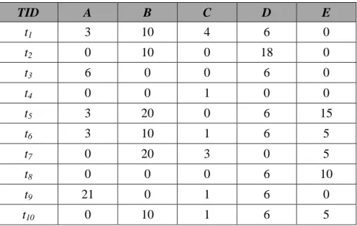
from a set of transactions. Assume the ten transactions shown in Table 4 are used for
mining. Each transaction consists of two features, transaction identification (TID) and
Table 4: The set of ten transaction data for this example. TID A B C D E t1 1 1 4 1 0 t2 0 1 0 3 0 t3 2 0 0 1 0 t4 0 0 1 0 0 t5 1 2 0 1 3 t6 1 1 1 1 1 t7 0 2 3 0 1 t8 0 0 0 1 2 t9 7 0 1 1 0 t10 0 1 1 1 1
Also assume that the predefined profit value for each single item is defined in Table 5.
Table 5: The predefined profit values of the items. Item Profit A 3 B 10 C 1 D 6 E 5
Moreover, the minimum average-utility threshold
λ
is set as 45.4 which is 20% oftotal utility. In order to find the high average-utility itemsets from the data in Table 4,
the proposed mining algorithm proceeds as follows.
STEP 1: The utility value of each item occurring in each transaction in Table 4 is
transaction 7 is 2, and its profit is 10. The utility value of B is thus calculated as 2*10,
which is 20. The utility values of all the items in each transaction are shown in Table
6.
Table 6: The utility values of all the items in each transaction.
TID A B C D E t1 3 10 4 6 0 t2 0 10 0 18 0 t3 6 0 0 6 0 t4 0 0 1 0 0 t5 3 20 0 6 15 t6 3 10 1 6 5 t7 0 20 3 0 5 t8 0 0 0 6 10 t9 21 0 1 6 0 t10 0 10 1 6 5
STEP 2: The utility values of the items in each transaction are compared and the
maximal utility value in the transaction is found. Take transaction 1 as an example. It
can be observed from Table 6 that the utility value of B is 10, which is the maximal in
Table 7: The maximal utility values in each transaction of all the given ten transactions.
TID A B C D E Maximal Utility Value
in Transaction t1 3 10 4 6 0 10 t2 0 10 0 18 0 18 t3 6 0 0 6 0 6 t4 0 0 1 0 0 1 t5 3 20 0 6 15 20 t6 3 10 1 6 5 10 t7 0 20 3 0 5 20 t8 0 0 0 6 10 10 t9 21 0 1 6 0 21 t10 0 10 1 6 5 10
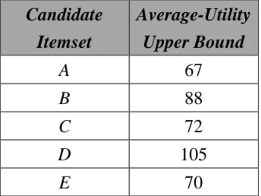
STEP 3: The average-utility upper bound of 1-itemsets is calculated. Take item A
as an example. It appears in transactions 1, 3, 5, 6 and 9. The average-utility upper
bound of A is thus the total amount of the maximal utility values of these transactions.
It is calculated as 10 + 6 + 20 + 10 + 21, which is 67. The upper-bound values of all
the items are shown in Table 8.
Table 8: The average-utility upper bounds of 1-itemsets. Candidate Itemset Average-Utility Upper Bound A 67 B 88 C 72 D 105 E 70
STEP 4: Check whether the average-utility upper bound of 1-itemsets is larger
than or equal to user-defined minimum average-utility threshold
λ
, which is 45.4. Inthis example, the average-utility upper bound of 1-itemsets exceeds the minimum
average-utility threshold
λ
. All the items are recorded as candidate average-utility1-itemsets, C1, shown in Table 9.
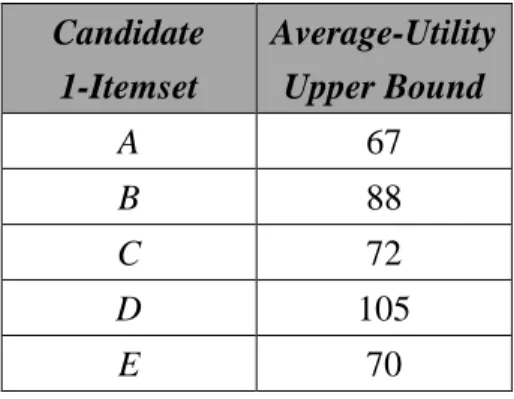
Table 9: The candidate average-utility 1-itemsets, C1.
Candidate 1-Itemset Average-Utility Upper Bound A 67 B 88 C 72 D 105 E 70
STEP 5: The variable r is set at 1, where r is used to represent the number of
items in the current candidate average-utility itemsets to be processed.
STEP 6: The candidate average-utility 2-itemsets (C2) are then generated from C1.
They are {AB}, {AC}, {AD}, {AE}, {BC}, {BD}, {BE}, {CD}, {CE}, {DE}.
STEP 7: The average-utility upper bound of each 2-itemset is calculated. Take
the itemset {AB} as an example. It appears in transactions 1, 5 and 6. The
average-utility upper bound of {AB} is thus the total amount of the maximal utility
values of these transactions as 10 + 20 + 10, which is 40. The upper-bound values of
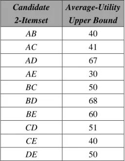
Table 10: The average-utility upper bounds of the 2-itemsets. Candidate 2-Itemset Average-Utility Upper Bound AB 40 AC 41 AD 67 AE 30 BC 50 BD 68 BE 60 CD 51 CE 40 DE 50
STEP 8: The average-utility upper bound of each 2-itemset is thus checked
against the user-defined minimum average-utility threshold λ. In this example, the
itemsets {AB}, {AC}, {AE} and {CE} do not exceed λ. These itemsets are thus
removed from C2. The remaining candidate average-utility 2-itemsets are shown in
Table 11.
Table 11: The remaining candidate average-utility 2-itemsets, C2.
Candidate 2-Itemset Average-Utility Upper Bound AD 67 BC 50 BD 68 BE 60 CD 51 DE 50
STEP 9: Since C2 is not null, r is incremented to 2 and STEPs 6 to 9 are repeated.
C3 is then generated from C2 as shown in Table 12.
Table 12: The average-utility upper bounds of the 3-itemsets Candidate 3-Itemset Average-Utility Upper Bound BCD 30 BDE 40
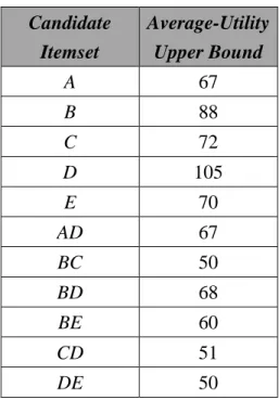
Since the average-utility upper bounds of both the two candidate 3-itemsets are
less than λ, they are removed from C3 and C3 becomes null. After this step, all the
candidate average-utility itemsets are shown in Table 13.
Table 13: All the candidate average-utility itemsets in the example. Candidate Itemset Average-Utility Upper Bound A 67 B 88 C 72 D 105 E 70 AD 67 BC 50 BD 68 BE 60 CD 51 DE 50
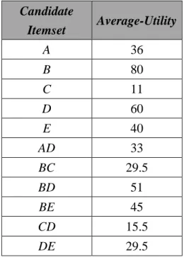
itemset is calculated. Take the itemset {AD} as an example. The actual utility values
of items A and D in transaction 1 are 3 and 6, respectively. Since the itemset {AD}
contains 2 items, its actual average-utility value in transaction 1 is calculated as (3 + 6)
/ 2, which is 4.5. The itemset {AD} appears in transactions 1, 3, 5, 6 and 9. The actual
average-utility value of {AD} is thus the total amount of actual average-utility
values of these transactions. The value is calculated as (9 + 12 + 9 + 9 + 27) / 2,
which is 33. The actual average-utility value of each candidate average-utility itemset
is shown in Table 14.
Table 14: The actual average-utility values of the candidate average-utility itemsets. Candidate Itemset Average-Utility A 36 B 80 C 11 D 60 E 40 AD 33 BC 29.5 BD 51 BE 45 CD 15.5 DE 29.5
STEP 11: The actual average-utility value of each candidate average-utility
itemset is then compared with the user-defined minimum average-utility threshold
λ
.larger than or equal to
λ
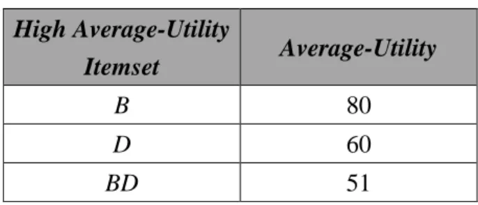
. They are thus put into the set of high average-utility itemsets,H, as shown in Table 15.
Table 15: High average-utility itemsets. High Average-Utility
Itemset Average-Utility
B 80
D 60
BD 51
In this example, four high average-utility itemsets are generated. Note that if the
traditional utility criterion is used, the results will be {B}, {D}, {AD}, {BC}, {BD},
{BE} and {DE}. The number of the high average-utility itemsets is less than that of
the high utility itemset. Under the perspective of the average utility, the utility values
of itemsets won’t increase with the increase of itemset length. The item combination
in a high average-utility itemset can thus really show its excellence in obtaining
profits.
6.
Experimental Results
Experiments were made to show the performance of the proposed approach. All the
experiments were performed on an Intel Core 2 Duo E6550 (2.33GHz) PC with 2 GB
main memory, running the Windows XP Professional operating system. The proposed
A real data set from a major grocery chain store in America was used for the
experiments. There were 21,556 transactions and 1,559 distinct items in the database.
Each transaction consisted of the products sold and their quantities. The average
transaction length was 4.03. The total utility from all the transactions in the dataset was
104,450,739. Figure 1 shows the number of candidate itemsets generated by our
proposed approach (TPAU) and Liu’s two-phased approach (TP), respectively. The
minimum utility threshold varied from 0.008% to 0.012%. From the figure, it could be
observed that TPAU generated much fewer candidate itemsets than TP did. The
number of candidate itemsets generated by TPAU decreased substantially. The
computation time could thus be greatly reduced.
0 50000 100000 150000 200000 250000 0.008% 0.009% 0.010% 0.011% 0.012% N u m b e r o f C a n d id a te I te m se ts
Minimum Utility Threshold
TPAU
TP
Figure 1. Numbers of candidate itemsets along with different minimum utility thresholds for the two approaches
Table 16 presents the summary of the numbers of candidate itemsets (CI), high
average-utility itemsets (HAUI) generated by our approach and high utility itemsets
(HUI) generated by Liu’s two-phased approach. In Phase I, TPAU generated much
fewer candidate itemsets than TP did. In Phase II, the number of high average-utility
itemsets (HAUI) was much less than that of high utility itemsets (HUI). TPAU could
discover high average-utility itemsets whose utility values were much closer to the
minimum utility threshold when compared to high utility itemsets.
Table 16: Comparison of the numbers of candidate itemsets (CI), high average-utility itemsets (HAUI) and high utility itemsets (HUI) of the two approaches.
Phase I Phase II
Threshold TPAU TP TPAU TP
CI CI HAUI HUI 0.012% 1583 37707 1556 3497 0.011% 1614 53324 1557 4557 0.010% 1677 80735 1565 6486 0.009% 1896 125920 1579 9997 0.008% 2288 197251 1605 18005
Figure 2 shows the execution time of the two approaches. The execution time of
0 500 1000 1500 2000 2500 3000 3500 0.008% 0.009% 0.010% 0.011% 0.012% E x e cu ti o n T im e (s e c. )
Minimum Utility Threshold
TPAU
TP
Figure 2. Execution time along with different minimum utility thresholds for the two approaches.
7.
Conclusions
This paper defines a new mining measure called average utility and proposes a
two-phase mining algorithm to discover high average-utility itemsets. The proposed
mining algorithm is divided into two phases. In phase I, this algorithm overestimates
the utility of itemsets for maintaining the “downward closure” property. The property
is then used to efficiently prune impossible utility itemsets level by level. In phase II,
one database scan is needed to determine the actual high average-utility itemsets from
the candidate itemsets generated in phase I. Since the number of candidate itemsets has
computational time may be saved. Considering that the length of itemsets is a major
factor to influence the utility values of itemsets in traditional approaches, the measure
“average-utility” is good to avoid the influence of the length. It can thus get a trade-off
between high utility and time complexity. The experimental results also show the
above points.
References
[1] R. Agarwal, C. Aggarwal, and V. Prasad, "A Tree Projection Algorithm
for Generation of Frequent Itemsets," Journal of Parallel and Distributed
Computing, vol. 61, pp. 350-371, 2001.
[2] R. Agrawal, T. Imielinski, and A. Swami, "Mining Association Rules
between Sets of Items in Large Databases," The 1993 ACM SIGMOD
International Conference on Management of Data, pp. 207-216, 1993.
[3] R. Agrawal and R. Srikant, "Fast Algorithms for Mining Association
Rules," The 20th International Conference on Very Large Data Bases, pp.
487-499, 1994.
[4] R. Agrawal and R. Srikant, "Mining Sequential Patterns," The 11th
International Conference on Data Engineering, pp. 3-14, 1995.
and Performance Improvements," The 5th International Conference on
Extending Database Technology, pp. 3-17, 1996.
[6] B. Barber and H. J. Hamilton, "Algorithms for Mining Share Frequent
Itemsets Containing Infrequent Subsets," Lecture Notes in Computer
Science, vol. 1910, pp. 76-99, 2000.
[7] B. Barber and H. Hamilton, "Extracting Share Frequent Itemsets with
Infrequent Subsets," Data Mining and Knowledge Discovery, vol. 7, pp.
153-185, 2003.
[8] F. Berzal, J. Cubero, N. Marin, and J. Serrano, "TBAR: An Efficient
Method for Association Rule Mining in Relational Databases," Data &
Knowledge Engineering, vol. 37, pp. 47-64, 2001.
[9] S. Brin, R. Motwani, J. D. Ullman, and S. Tsur, "Dynamic Itemset
Counting and Implication Rules for Market Basket Data," The 1997 ACM
SIGMOD International Conference on Management of Data, pp. 255-264,
1997.
[10] C. Chang and C. Lin, "Perfect Hashing Schemes for Mining Association
Rules," The Computer Journal, vol. 48, pp. 168-179, 2005.
[11] G. Grahne and J. Zhu, "Fast Algorithms for Frequent Itemset Mining
Engineering, vol. 17, pp. 1347-1362, 2005.
[12] J. Han, J. Pei, B. Mortazavi-Asl, Q. Chen, U. Dayal, and M.-C. Hsu,
"FreeSpan: Frequent Pattern-Projected Sequential Pattern Mining," The
6th ACM SIGKDD International Conference on Knowledge Discovery
and Data Mining, pp. 355-359, 2000.
[13] J. Han, J. Pei, Y. Yin, and R. Mao, "Mining Frequent Patterns without
Candidate Generation: A Frequent-Pattern Tree Approach," Data Mining
and Knowledge Discovery, vol. 8, pp. 53-87, 2004.
[14] K. Hu, Y. Lu, L. Zhou, and C. Shi, "Integrating Classification and
Association Rule Mining: A Concept Lattice Framework," Lecture Notes
In Computer Science, vol. 1711, pp. 443-447, 2004.
[15] H. Jiawei, P. Jian, and Y. Yiwen, "Mining Frequent Patterns without
Candidate Generation," The ACM SIGMOD International Conference on
Management of Data, pp. 1-12, 2000.
[16] L. Junqiang, P. Yunhe, W. Ke, and H. Jia-wei, "Mining Frequent Item
Sets by Opportunistic Projection," The 8th ACM SIGKDD International
Conference on Knowledge Discovery and Data Mining, pp. 229-238,
2002.
Frequent Itemsets," Lecture notes in computer science vol. 3309, pp.
266-277, 2004.
[18] Y. Li, J. Yeh, and C. Chang, "Direct Candidates Generation: A Novel
Algorithm for Discovering Complete Share-Frequent Itemsets," Lecture
Notes in Computer Science, vol. 3614, p. 551, 2005.
[19] Y. Li, J. Yeh, and C. Chang, "Efficient Algorithms for Mining
Share-Frequent Itemsets," The 11th World Congress of International
Fuzzy Systems Association, pp. 543-539, 2005.
[20] Y. Li, J. Yeh, and C. Chang, "A Fast Algorithm for Mining
Share-Frequent Itemsets," The 7th Asia Pacific Web Conference, pp.
417-428, 2005.
[21] Y. Liu, W.-k. Liao, and A. Choudhary, "A Two-Phase Algorithm for Fast
Discovery of High Utility Itemsets," Lecture Notes in Computer Science,
vol. 3518, pp. 689-695, 2005.
[22] Y. Liu, W. Liao, and A. Choudhary, "A Fast High Utility Itemsets Mining
Algorithm," The 1st International Workshop on Utility-Based Data
Mining, pp. 90-99, 2005.
[23] J. Park, M. Chen, and P. Yu, "An Effective Hash-Based Algorithm for
Conference on Management of Data, pp. 175-186, 1995.
[24] Y. G. Sucahyo and R. P. Gopalan, "Building a More Accurate Classifier
Based on Strong Frequent Patterns," Lecture Notes in Computer Science,
vol. 3339, pp. 1036-1042, 2005.
[25] H. Yao, H. Hamilton, and C. Butz, "A Foundational Approach to Mining
Itemset Utilities from Databases," The 4th SIAM International
Conference on Data Mining, pp. 211-225, 2004.
[26] H. Yao and H. Hamilton, "Mining Itemset Utilities from Transaction
Databases," Data & Knowledge Engineering, vol. 59, pp. 603-626, 2006.
[27] M. Zaki, S. Parthasarathy, M. Ogihara, and W. Li, "New Algorithms for
Fast Discovery of Association Rules," The 3rd International Conference