Solving the K-of-N Lifetime Problem by PSO

(1)

MultiCraft International Journal of Engineering, Science and Technology

Solving the K-of-N Lifetime Problem by PSO

Tzung-Pei Hong

1, 2

and Guo-Neng Shiu

3 1

Department of Computer Science and Information Engineering National University of Kaohsiung, Kaohsiung, 811, Taiwan

2_{Department of Computer Science and Engineering National Sun Yat-sen University, Kaohsiung, 804, Taiwan}

3_{Department of Electrical Engineering National University of Kaohsiung, Kaohsiung, 811, Taiwan}

e-mail:tphong@nuk.edu.tw, lunasea.deen@msa.hinet.net

Abstract

In wireless sensor networks, application nodes (ANs) may be produced by different manufacturers and may own different data transmission rates, initial energies and parameter values. When different kinds of ANs exist in a wireless network, it is hard to find the optimal base-station (BS) locations for minimizing power consumption and prolonging network lifetime. In this paper, a heuristic algorithm based on PSO is thus proposed to solve the K-of-N lifetime problem under general power-consumption constraints in wireless sensor networks. Give N ANs, the network survives as long as there are at least K ANs alive. The proposed approach can search for nearly optimal BS locations in heterogeneous sensor networks, where application nodes may own different data transmission rates, initial energies and parameter values. Experimental results also show the good performance of the proposed PSO approach and the effects of the parameters on the results. The proposed algorithm can thus help maximize the K-of-N network lifetime in wireless sensor networks.

Keywords: wireless sensor network, network lifetime, energy consumption, particle swarm optimization

1. Introduction

In a wireless sensor network, sensor nodes (SNs) are usually small, low-cost and disposable, and do not communicate with other sensor nodes. They are usually deployed in clusters around interesting areas. Each cluster of sensor nodes is allocated with at least one application node. Application nodes (ANs) possess longer-range transmission, higher-speed computation, and more energy than sensor nodes. The raw data obtained from sensor nodes are first transmitted to their corresponding application nodes. After receiving the raw data from all its sensor nodes, an application node conducts data fusion within each cluster. It then transmits the aggregated data directly to the base station or via multi-hop communication. The base station (BS) is usually assumed to have unlimited energy and powerful processing capability. It also serves as a gateway for wireless sensor networks to exchange data and information to other networks. Wireless sensor networks usually have some assumptions for SNs and ANs. For instance, each AN may be aware of its own location through receiving GPS signals [11] and its own energy.

A fundamental problem in wireless sensor networks is to prolong the system lifetime under some given constraints. In the past, many approaches were proposed to efficiently utilize energy in wireless networks. For example, appropriate transmission ways were designed to save energy for multi-hop communication in ad-hoc networks [16][10][5][19][7][6][21]. Good algorithms for allocation of base stations and sensors nodes were also proposed to reduce power consumption [12][15][16][8][9]. Pan et al. proposed several algorithms to find the optimal locations of base stations in two-tiered wireless sensor networks [13]. Their approaches assumed the initial energy and the energy-consumption parameters were the same for all ANs. If any of the above parameters were not the same, their approaches could not work.

Recently, the technique of particle swarm optimization (PSO) technique has been widely used in finding nearly optimal solutions for optimization problems [1][2][20]. Finding BS locations is by nature very similar to finding the food locations originated from PSO. In the past, we proposed a PSO-based approach to allocate base stations for the N-of-N problem in which

(2)

lifetime problem under general power-consumption constraints in wireless sensor networks. Give N ANs, the network survives as long as there are at least K ANs alive. The proposed approach can search for nearly optimal BS locations in heterogeneous sensor networks, where application nodes may own different data transmission rates, initial energies and parameter values. Pan et al.’s extension from solving the N-of-N problem to solving the K-of-N problem was a little complicated. The extension by the proposed PSO approach is, however, very easy. Besides, the proposed approach can handle different initial energy and energy-consumption parameters, which cannot be processed in Pan et al.’s approach. Extensive experiments are also made to show the performance of the proposed PSO approach for the K-of-N lifetime problem and the effects of the parameters on the results.

The remaining parts of this paper are organized as follows. Some related works about finding the locations of base stations in a two-tiered wireless networks is reviewed in Section 2. The PSO approach is introduced in Section 3. An algorithm based on PSO to solve the K-of-N lifetime problem in a two-tiered wireless network is proposed in Section 4. A small example to illustrate the approach is given in Section 5. Experimental results for demonstrating the performance of the algorithm and the effects of the parameters are described in Section 6. Conclusions are stated in Section 7.

2. Review of Related Works

As mentioned above, a fundamental problem in wireless sensor networks is to maximize the system lifetime under some given constraints. Pan et al. first proposed an algorithm to find the optimal locations of base stations in two-tiered wireless homogeneous sensor networks [13] for the N-of N problem. Give N ANs, the mission failed when any of the N ANs ran out of energy. Let d be the Euclidean distance from an AN to a BS, and r be the data transmission rate. Pan et al. adopted the following formula to calculate the energy consumption per unit time:

), ( ) , ( 1 2 n d r d r p =

α

+

α

where α1 was a distance-independent parameter and α2 was a distance-dependent parameter. The energy consumption thus related to Euclidean distances and data transmission rates. Pan et al. assumed each AN had the same α1, α2 and initial energy. For homogenous ANs, they showed that the center of the minimal circle covering all the ANs was the optimal BS location (with the maximum lifetime) for the N-of-N condition.

Pan et al. then proposed an approach to find the optimal locations of base stations for the K-of-N problem [13]. Give N ANs, the mission survived as long as there were at least K ANs alive, or the mission failed when N-K+1 ANs ran out of energy. Pan et al.’s approach for the K-of-N problem was a little complicated when compared to that for the N-of-N problem. It first used the N-of-N approach to find a minimal circle covering all the ANs. Each minimum circle would have at least two ANs (or three if the ANs were not on the diameter) on the circumference according to the property of circles. The approach then found the (N-1)-of-N lifetime by removing any one point on the circumference. If there were R points on the circumference, then R possible circles would be found, each as a possible (N-1)-of-N result. The approach then found the (N-2)-of-N lifetime by removing one more ANs from the (N-1)-of-N circles. The same procedure was repeated until only N-K ANs remained in the network. The approach then selected the minimum circle. A smaller circle represented that the system had a larger lifetime.

Pan et al. also extended their approaches to find the optimal BS location for ANs with different transmission rates by using stacked planes [13]. But if the application nodes own different data transmission rates, initial energies and parameter values, their approaches can not work.

3. Review of Particle Swarm Optimization

The PSO technique was proposed by Eberhart and Kennedy in 1995 [1][2] and has been widely used in finding solutions for optimization problems. Some related researches about its improvement and applications has also been proposed [3][14][17][18]. It maintains several particles (each represents a solution) and simulates the behavior of bird flocking to find the final solutions. All the particles continuously move in the search space, tending to better solutions, until the termination criteria are met. After a lot of generations, the optimal solution or an approximate optimal solution is expected to be found.

Suppose there is a group of birds searching for food in an area. Also assume each bird has the instinct of remembering its own location with the most food in its experience. Besides, all the birds can exchange their best experiences to each other and thus learn the location with the most food found so far in the search space. Each bird thus knows both the best location in its experience and the best one from the flock of birds, and will tend to move according to the two locations. The PSO approach thus simulates the mentioned behaviors of bird flocking to find solutions of optimization problems.

When the PSO technique is used to solve a problem, each possible solution in the search space is called a particle, which is similar to a bird mentioned above. All the particles are evaluated by a fitness function, with the values representing the goodness degrees of the solutions. The solution with the best fitness value for a particle can be regarded as the local optimal solution found so far and is stored as the pBest solution for the particle. The best one among all the pBest solutions is regarded as the global optimal solution found so far for the whole set of particles, and is called the gBest solution. In addition, each particle moves with a velocity, which will dynamically change according to pBest and gBest. After finding the two best values, a particle updates its velocity by the following equation:

(3)

), ( ) ( ) ( ) ( _id _id ₂ ₂ _d _id 1 1 old id new

id w V c Rand pBest x c Rand gBest x

V = × + × × − + × × −

where the terms are explained below. 1. new

id

V : the velocity of the i-th particle in the d-th dimension in the next generation; 2. old

id

V : the velocity of the i-th particle in the d-th dimension in the current generation; 3. pBestid: the current pBest value of the i-th particle in the d-th dimension;

4. gbestd: the current gBest value of the whole set of particles in the d-th dimension; 5. xid: the current position of the i-th particle in the d-th dimension;

6. w: the inertial weight, generally set at 1 [17];

7. c1: the acceleration constant for a particle to move to its pBest, generally set at 2 [2]; 8. c2: the acceleration constant for a particle to move to the gBest, generally set at 2 [2]; 9. Rand1(), Rand2(): two random numbers within 0 to 1.

After the new velocity is found, the new position for a particle can then be obtained by the following formula:

.

new id id id

x

V

x

=

+

All the particles thus continuously move in the search space, tending to better solutions, until the termination criteria are met. After a lot of generations, an approximate optimal solution is expected to be found. The PSO algorithm is stated below.

4. Using the PSO Algorithm to Solve the K-of-N Lifetime Problem

The ANs produced by different manufacturers may own different data transmission rates, initial energies and parameter values. When different kinds of ANs exist in a wireless network, it is hard to find the optimal BS location. In this section, a heuristic algorithm based on PSO to solve the K-of-N lifetime problem under general constraints is proposed. An initial set of particles is first randomly generated, with each particle representing the coordinate of a possible BS location. Each particle is also allocated an initial velocity for changing its state. Let ej(0) be the initial energy, rj be the data transmission rate, αj1 be the distance-independent parameter, and αj2 be the distance-dependent parameter of the j-th AN. The lifetime lij of an application node ANj for the i-th particle is calculated by the following formula:

, ) ( ) 0 ( n ij j j j j ij e r d l = α +α where n ij

d is the n-order Euclidian distance from the j-th AN to the i-th particle. In the K-of-N lifetime problem, given N ANs, the system survives as long as at least K ANs are alive. Restated, the system fails when at least N-K+1 ANs run out of energy. The fitness function used for evaluating each particle is thus shown below:

}. { ) ( ₁ 1 N K ij N j l Min i fitness ₋ ₊ = = That is, the fitness of the i-th particle is its (N-K+1)-th minimal lifetime among all the ANs. A larger fitness value thus denotes a better solution quality for the K-of-N lifetime problem, meaning the corresponding BS location is better. The fitness value of each particle is then compared with that of its corresponding pBest. If the fitness value of the i-th particle is larger than that of pBesti,

pBesti is replaced with the i-th particle. The best pBesti among all the particles is chosen as the gBest. Besides, each particle has a velocity, which is used to change the current position. All particles thus continuously move in the search space. When the termination conditions are achieved, the final gBest will be output as the location of the base station. The proposed algorithm is stated below.

The proposed PSO algorithm for the K-of-N lifetime problem:

Input: A set of N ANs, each ANj with its location (xj, yj), data transmission rate rj, initial energy ej(0), parameter αj1, parameter αj2, and the allowed number K of alive ANs.

Output: A BS location that will cause a nearly maximal lifetime for the K-of-N lifetime problem. Step 1: Initialize the fitness values of all pBests and the gBest to zero.

Step 2: Randomly generate a group of n particles, each representing the coordinate of a possible BS location. Locations may be two-dimensional or three-dimensional, depending on the problems to be solved.

Step 3: Randomly generate an initial velocity for each particle.

Step 4: Calculate the lifetime lij of the j-th AN for the i-th particle by the following formula: ), ( ) 0 ( _j _j₁ _j₂ _ijn j ij e r d l = α +α

where ej(0) is the initial energy, rj is the data transmission rate, αj1 is a distance-independent parameter, αj2 is a distance-dependent parameter of the j-th AN, and n

ij

d _{is the n-order Euclidean distance from the i-th particle (BS) to the j-th AN.} Step 5: Calculate the (N-K+1)-th minimal lifetime among all the ANs for the i-th particle as its fitness value (fitness(i)) by the

(4)

}, { ) ( 1 1 N K ij N j l Min i fitness ₋ ₊ = =

where N is number of ANs, K is the allowed number of alive ANs, i = 1 to n, and j=1 to N.

Step 6: Set pBesti as the current i-th particle if the value of fitness(i) is larger than the current fitness value of pBesti. Step 7: Set gBest as the best pBest among all the particles. That is, let:

fitness of pBestk = n i

max =1fitness of pBesti, and set gBest=pBestk.

Step 8: Update the velocity of the i-th particle as:

), ( ) ( ) ( ) ( id id 2 2 d id 1 1 old id new

id w V c Rand pBest x c Rand gBest x

V = × + × × − + × × −

where Vidnew is the new velocity of the i-th particle at the d-th dimension,

old id

V is the current velocity of the i-th particle at the d-th dimension, w is the inertial weight, c1 is the acceleration constant for particles moving to pBest, c2 is the acceleration constant for particles moving to gBest, Rand1( ) and Rand2( ) are two random numbers among 0 to 1, xid is the current position of the i-th particle at the d-th dimension, pBestid is the value of pBesti at the d-th dimension, and gBestd is the value of gBest at the d-th dimension.

Step 9: Update the position of the i-th particle as:

, new id old id new id x V x = +

where

x

idnew and old id

x are respectively the new position and the current position of the i-th particle at the d-th dimension. Step 10: Repeat Steps 4 to 9 until the termination conditions are satisfied.

In Step 10, the termination conditions may be predefined execution time, a fixed number of generations or when the particles have converged to a certain threshold.

5. A Small Example

In this section, a simple example in a two-dimensional space is given to explain how the PSO approach can be used to find the best BS location for the K-of-N lifetime problem. Assume there are totally four ANs in the example and their initial parameters are shown in Table 1, where “Location” represents the two-dimensional coordinate position of an AN, “Rate” represents the data transmission rate, and “Power” represents the initially allocated energy. All αj1’s are set at 0 and all αj2’s at 1 for simplicity. Also assume the allowed number K of alive ANs is 3.

Table 1: The initial parameters of ANs in the example

Assume 3 particles are used for simplicity. Also assume the three initial particles randomly generated are located at (4, 7), (9, 5) and (6, 4). An initial velocity is randomly generated for each particle. In this example assume the initial velocity is set at zero for simplicity. The lifetime of each AN for a particle is then calculated. Take the first AN for the first particle as an example. Its lifetime is calculated as follows:

18 . 185 ] ) 10 7 ( ) 1 4 [( 3 10000 2 2 11= − + − = l .

The lifetimes of all ANs for all particles are shown in Table 2.

Table 2: The lifetimes of all ANs for all particles 1(1, 10) 2(11, 0) 3(8, 7) 4(4, 3) 1(4, 7) 185.18 20.40 100 100 2(9, 5) 37.45 68.96 320 55.17 3(6, 4) 54.64 48.78 123.07 320

The (N-K+1)-th minimal lifetime among all the ANs for each particle is calculated as its fitness value. The results are 100, 55.17 and 54.64 for the three particles. The fitness value of each particle is then compared with that of its corresponding pBest. In the first generation, the fitness values of all the pBests are zero, smaller than those of the particles. The particles are then stored as the

AN Location Rate Power 1 (1, 10) 3 10000 2 (11, 0) 5 10000

3 (8, 7) 4 6400

4 (4, 3) 4 6400

(5)

new pBests. The best pBest among all the particles is chosen as the gBest. In this example, the first particle is set as the gBest. The new velocity and the position of each particle are then updated. Steps 4 to 9 are then repeated until the termination conditions are satisfied. In this example, the solutions converge after about 70 generations. The solution was located at (4.5515, 6.419) and its lifetime was 130.8344 time units.

6. Experimental Results

Experiments were made to show the performance of the proposed PSO algorithm on finding optimal base stations for the K-of-N lifetime problem. They were performed in C language on an AMD PC with a 2.0GHz processor and 1G main memory and running the Microsoft Window XP operating system. The simulation was done in a two-dimensional real-number space of 1000*1000. That is, the ranges for both x and y axes were between 0 to 1000. The data transmission rate was limited between 1 to 10 and the range of initial energy was limited between 100000000 to 999999999. The data of all ANs, each with its own location, data transmission rate and initial energy, were randomly generated.

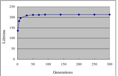
Experiments were first made to show the convergence of the proposed PSO algorithm when the acceleration constant (c1) for a particle moving to its pBest was set at 2, the acceleration constant (c2) for a particle moving to its gBest was set at 2, the inertial weight (w) was set at 0.6, the distance-independent parameter (αj1) was set at zero, and the distance-dependent parameter (αj2) was set at one. Assume totally there were 50 ANs in the system and the allowed number (K) of alive ANs was set at 40. The experimental results of the resulting lifetime along with different generations for 10 particles in each generation are shown in Figure 1. 0 50 100 150 200 250 0 50 100 150 200 250 300 Generations L if e ti m e

Figure 1. The lifetime for the 40-of-50 lifetime problem and10 particles

It is easily seen from Figure 1 that the proposed PSO algorithm could converge very fast (at about 50 generations). Next, experiments were made to show the effects of different parameters on the K-of-N lifetime problem. The influence of the acceleration constant (c1) for a particle moving to its pBest on the proposed algorithm was first considered. The process was terminated at 300 generations. When w = 1 and c2 = 2, the lifetimes along with different acceleration constants (c1) are shown in Figure 2.

(6)

200 201 202 203 204 205 206 0 1 2 3 4 c1 L if et im e

Figure 2. The lifetimes along with different acceleration constants (c1)

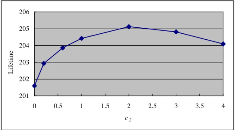
It can be observed from Figure 2 that the lifetime first increased and then decreased along with the increase of the acceleration constant (c1). It was because when the value of the acceleration constant (c1) was small, the velocity update of each particle was also small, causing the convergence speed slow. The proposed PSO algorithm might thus not get the optimal solution after the predefined number of generations. On the contrary, when the value of the acceleration constant (c1) was large, the velocity change would be large as well, causing the particles to move fast. It was then hard to converge. In the experiments, the optimal c1 value was about 2. Next, experiments were made to show the effects of the acceleration constant (c2) for a particle moving to its gBest on the proposed algorithm. When w = 1 and c1 = 2, the experimental results are shown in Figure 3.

201 202 203 204 205 206 0 0.5 1 1.5 2 2.5 3 3.5 4 c2 L if et im e

Figure 3. The lifetimes along with different acceleration constants (c2)

It can be observed from Figure 3 that the lifetime first increased and then decreased along with the increase of the acceleration constant (c2). The reason was the same as above. In the experiments, the optimal c2 value was about 2. Next, experiments were made to show the effects of the inertial weight (w) on the proposed algorithm. When c1 = 2 and c2 = 2, the experimental results are shown in Figure 4.

(7)

185 190 195 200 205 210 215 0 0.5 1 1.5 2 2.5 3 w L if et im e

Figure 4. The lifetimes along with different inertial weights (w)

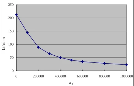
It can be observed from Figure 4 that the proposed algorithm could get better lifetime when the inertial weight (w) was smaller than 0.6. The lifetime decreased along with the increase of the inertial weight (w) when w was bigger than 0.6. This was because when the value of the inertial weight was large, the particles would move fast due to the multiple of the old velocity. It was then hard to converge. Experiments were then made to show the effects of the distance-independent parameter (α1) on the lifetime. In the experiments, all ANs had the same value of the distance-independent parameter. The experimental results are shown in Figure 5. 0 50 100 150 200 250 0 200000 400000 600000 800000 1000000 α₁ L if et im e

Figure 5. The lifetimes along with different values of the distance-independent parameter (α1)

It can be observed from Figure 5 that the lifetime decreased along with the increase of the value of the distance-independent parameter (α1). The relation was nearly linear. It was consistent with the formula of energy consumption. Next, experiments were made to show the effects of the distance-dependent parameter (α2) on the lifetime. The experimental results are shown in Figure 6.

(8)

0 50 100 150 200 250 0 1 2 3 4 5 α₂ L if et im e

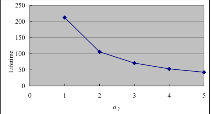
Figure 6. The lifetimes along with different values of the distance-dependent parameter (α2)

It can be observed from Figure 6 that the lifetime decreased along with the increase of the distance-dependent parameter (α2). It was also consistent with the formula of energy consumption. Besides, the relation between the lifetime and the value of the distance-dependent parameter presented an approximately inverse proportion. Next, experiments were made to show the relation between lifetimes and numbers of ANs. The experimental results are shown in Figure 7.

0 100 200 300 400 500 600 700 800 40 50 60 70 80 90 100 ANs L if et im e

Figure 7. The lifetimes along with different numbers of ANs

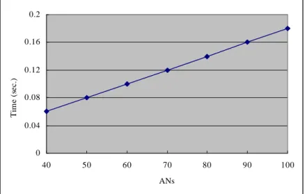
It can be seen from Figure 7 that the lifetime increased along with the increase of the number of ANs. The execution time along with different numbers of ANs is shown in Figure 8.

(9)

0 0.04 0.08 0.12 0.16 0.2 40 50 60 70 80 90 100 ANs T im e (s e c. )

Figure 8. The execution time along with different numbers of ANs

It can be observed from Figure 8 that the execution time increased along with the increase of numbers of ANs. The relation was nearly linear. Next, experiments were then made to show the relation between lifetimes and numbers of particles for 50ANs. The experimental results for w = 1 are shown in Figure 9.

206.5 207 207.5 208 208.5 209 209.5 210 210.5 211 211.5 0 20 40 60 80 100 Particles L if et im e

Figure 9. The lifetimes along with different numbers of particles

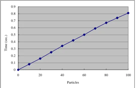
It can be seen from Figure 9 that the lifetime increased along with the increase of the number of particles. The execution time along with different numbers of particles is shown in Figure 10.

(10)

0 0.1 0.2 0.3 0.4 0.5 0.6 0.7 0.8 0.9 0 20 40 60 80 100 Particles T im e ( se c. )

Figure 10. The execution time along with different numbers of particles for 50 ANs

It can be observed from Figure 10 that the execution time increased along with the increase of numbers of particles. The relation would be nearly linear. This was reasonable since the execution time would be approximately proportional to the number of particles.

When implementing the particle swarm algorithm, several considerations must be taken into account to facilitate the convergence and prevent an explosion of the swarm. These considerations include limiting the maximum velocity, selecting acceleration constants, the constriction factor, or the inertia weight. A detailed discussion can be found in [20].

Note that no optimal solutions can be found in a finite amount of time since the problem is NP-hard. For a comparison, an exhaustive search using grids was used to find nearly optimal solutions. The approach found the lifetime of the system when a BS was allocated at any cross-point of the grids. The cross-point with the maximum lifetime was then output as the solution. A lifetime comparison of the PSO approach and the exhaustive search with different grid sizes are shown in Table 3.

Table 3. A lifetime comparison of the PSO approach and the exhaustive grid search

Method Lifetime

The proposed PSO algorithm 212.4404 The exhaustive grid search

(grid size = 1) 212.0781 The exhaustive grid search

(grid size = 0.1) 212.4158 The exhaustive grid search

(grid size = 0.01) 212.4379

It can be observed from Table 3 that the lifetime obtained by the proposed PSO algorithm was better than those by the exhaustive grid search with grid sizes larger than 0.01. The lifetime by the proposed PSO algorithm was 212.4404, and was 212.0781, 212.4158 and 212.4379 by the exhaustive search for the grid size respectively set at 1, 0.1 and 0.01. For the exhaustive grid search, the smaller the grid size, the better the results. The execution time by the two approaches is shown in Table 4.

Table 4. A comparison of execution time by the two approaches

Method Time (sec.)

The proposed PSO algorithm 0.06 The exhaustive grid search

(grid size = 1) 36.563 The exhaustive grid search

(grid size = 0.1) 2480.718 The exhaustive grid search

(11)

It can be seen from Table 4 that the execution time of the exhaustive grid search increased along with the decrease of grid sizes. It was very consistent with the processing way of the exhaustive grid search. Besides, the exhaustive grid search spent much more execution time than the proposed PSO algorithm, especially when the grid size was small. The advantage of the proposed PSO approach for solving the problem lies in that it can reduce the computation time and keep the same good quality.

7. Conclusion and Future Works

In wireless sensor networks, minimizing power consumption to prolong network lifetime has always been very crucial. In this paper, we have thus extended our previous approach to solve the K-of-N lifetime problem under general power-consumption constraints in wireless sensor networks. Finding BS locations is by nature very similar to finding the food locations originated from PSO. It is thus easy to model such a problem by the proposed algorithm based on PSO. The extension from solving the

N-of-N problem to solving the K-of-N-of-N problem by the proposed PSO approach is also very simple when compared to Pan et al.’s

extension.

The proposed approach can solve the K-of-N lifetime problem in heterogeneous sensor networks, where application nodes may own different data transmission rates, initial energies and parameter values. Extensive experiments have also been made to show the performance of the proposed PSO approach for the K-of-N lifetime problem and the effects of the parameters on the results. From the experimental results, it can be easily concluded that the proposed PSO algorithm converges very fast. Besides, the lifetime first increases and then decreases along with the increase of the acceleration constants c1, c2 and w. It also increases along with the increase of ANs, decreases along with the increase of the parameters α1 and α2, and decreases along with the decrease of particles. The execution time, however, increases in a nearly linear way along with the increase of ANs and particles. Note that if the problem to be solved is the ANs with the same initial energy and the same energy-consumption parameters, it is fine to use Pan et al.’s approach. Their approach spends polynomial time and can get the optimal solution. In the future, we will attempt to combine other approaches to automatically adjust the parameters.

Acknowledgement

This research was supported by the National Science Council of the Republic of China under contract NSC 982221E390 -033.

References

[1] R. C. Eberhart and J. Kennedy, “A new optimizer using particles swarm theory,” The Sixth International Symposium on

Micro Machine and Human Science, 1995, pp. 39-43.

[2] R. C. Eberhart and J. Kennedy, “Particle swarm optimization,” The IEEE International Conference on Neural Networks, Vol. 4, 1995, pp. 1942-1948.

[3] Z. L. Gaing, “Discrete particle swarm optimization algorithm for unit commitment,” The IEEE Power Engineering Society

General Meeting, 2003.

[4] T.P. Hong and G.N. Shiu, “A PSO-based heuristic algorithm for base-station locations,” International Conference on Soft

Computing and International Symposium on advanced Intelligent Systems (SCIS&ISIS 2006).

[5] W. Heinzelman, J. Kulik, and H. Balakrishnan, “Adaptive protocols for information dissemination in wireless sensor networks,” The Fifth ACM International Conference on Mobile Computing and Networking, pp. 174-185, 1999.

[6] W. Heinzelman, A. Chandrakasan, and H. Balakrishnan, “Energy-efficient communication protocols for wireless microsensor networks,” The Hawaiian International Conference on Systems Science, 2000.

[7] C. Intanagonwiwat, R. Govindan and D. Estrin, “Directed diffusion: a scalable and robust communication paradigm for sensor networks,” The ACM International Conference on Mobile Computing and Networking, 2000.

[8] Vikas Kawadia and P. R. Kumar, “Power control and clustering in ad hoc networks,” The 22nd IEEE Conference on

Computer Communications (INFOCOM), 2003.

[9] N. Li, J. C. Hou and L. Sha, “Design and analysis of an mst-based topology control algorithm,” The 22nd IEEE Conference

on Computer Communications (INFOCOM), 2003.

[10] S. Lee, W. Su and M. Gerla, “Wireless ad hoc multicast routing with mobility prediction,” Mobile Networks and

Applications, Vol. 6, No. 4, pp. 351-360, 2001.

[11] D. Niculescu and B. Nath, “Ad hoc positioning system (APS) using AoA,” The 22nd IEEE Conference on Computer

Communications (INFOCOM), pp. 1734-1743, 2003.

[12] J. Pan, Y. Hou, L. Cai, Y. Shi and X. Shen, “Topology control for wireless sensor networks,” The Ninth ACM International

Conference on Mobile Computing and Networking, pp. 286-299, 2003.

[13] J. Pan, L. Cai, Y. T. Hou, Y. Shi and S. X. Shen, "Optimal base-station locations in two-tiered wireless sensor networks,"

IEEE Transactions on Mobile Computing, Vol. 4, No. 5, pp. 458-473, 2005.

(12)

mutation operator,” The IEEE Third International Conference on Machine Learning and Cybernetics, pp. 2473-2478 2004. [15] V. Rodoplu and T. H. Meng, “Minimum energy mobile wireless networks,” IEEE Journal on Selected Areas in

Communications, Vol. 17, No. 8, 1999.

[16] R. Ramanathan and R. Hain, “Topology control of multihop wireless networks using transmit power adjustment,” The 19th

IEEE Conference on Computer Communications (INFOCOM), 2000.

[17] Y. Shi and R. C. Eberhart, “A modified particle swarm optimizer,” The IEEE International Conference on Evolutionary

Programming, 1998, pp. 69-73.

[18] A. Stacey, M. Jancic and I. Grundy, “Particle swarm optimization with mutation,” The IEEE Congress on Evolutionary

Computation, 2003, pp. 1425-1430.

[19] D. Tian and N. Georganas, “Energy efficient Routing with guaranteed delivery in wireless sensor networks,” The IEEE

Wireless Communication & Networking Conference, 2003.

[20] Y. del Valle, G. K. Venayagamoorthy, S. Mohagheghi, J. C. Hernandez and R. G. Harley, “Particle swarm optimization: basic concepts, variants and applications in power systems,” IEEE Transactions on Evolutionary Computation, Vol. 12, No. 2, 2008, pp. 171-195.

[21] F. Ye, H. Luo, J. Cheng, S. Lu and L. Zhang, “A two-tier data dissemination model for large scale wireless sensor networks,” The ACM International Conference on Mobile Computing and Networking, 2002.