國立交通大學
統計學研究所
碩士論文
AIC、BIC 和 EBIC 之回顧
Review of AIC, BIC and EBIC
研 究 生:顏妤樺
指導教授:洪慧念 教授
AIC、BIC 和 EBIC 之回顧
Review of AIC, BIC and EBIC
研究生:顏妤樺
Student: Yu-Hua Yen
指導教授:洪慧念 博士
Advisor: Dr. Hui-Nien Hung
國立交通大學理學院 統計學研究所 碩士論文 A Thesis Submitted to Institute of Science National Chiao Tung University in Partial Fulfillment of the Requirements
for the Degree of Master
in Statistics June 2014
Hsinchu, Taiwan, Republic of China
AIC、BIC 和 EBIC 之回顧
研究生:顏妤樺
指導教授:洪慧念 博士
國立交通大學統計學研究所碩士班
摘 要 自資訊爆炸以來,利用統計方法分析資料漸漸成為一種常態。而我們所面對的 問題也從過去的大樣本資料分析逐漸轉變成高維度資料分析。如何找出這些資料的 最適模型是我們最重要的課題。在這篇文章中,我們將 Chen & Chen (2008) 提出 之針對高維度模型選取方法 EBIC 與常見的模型選取方法 AIC、BIC 做比較,並 利用模擬的方式說明這些方法的差異與優劣。Review of AIC, BIC and EBIC
Student: Yu-Hua Yen
Advisor: Dr. Hui-Nien Hung
Institute of Statistics
National Chiao Tung University
Hsinchu 30010, Taiwan
Abstract
Since the information explosion, analyzing data by using statistical methods pro-gressively becomes norm. Nowadays, the problem we are faced with large sample size analysis gradually transformed into high dimensional model analysis. How to find the optimal model for the data is our most important issue. In our study, we compare EBIC, which proposed by Chen & Chen (2008) for high dimensional model, with common model selection methods, AIC and BIC, and use simulations illustrating the difference and the pros and cons of these methods.
誌 謝
首先,誠摯的感謝我的指導教授 洪慧念博士,感謝老師在指導我的論文上所花 費的時間與精力,並且不時的指點與引導我正確的研究方向,在這個過程中,除了更瞭 解模型選擇的方法之外,我學到了一件最重要的事:透過舉例的方式將抽象的概念具 體表達出來。另外,感謝口試委員 徐南蓉教授、黃信誠教授和王維菁教授的建議與指 教,使得本論文更為完整。 兩年裡的日子,研究室裡共同的生活點滴,學術上的討論、言不及義的閒扯、趕作 業的革命情感等,感謝所有同學的互相勉勵,因為有你們讓兩年的研究所生活變得絢 麗許多,恭喜我們都順利走過這兩年並且即將畢業。 感謝好友賴怡方、白永馨、徐光縈無時無刻給予我心靈上最強大的支持,也感謝室 友邱晴瑜、劉晏羽與我交流他們在各自的領域上對各種人事物的想法與觀點,讓我的 思維更加的多元化,另外特別感謝過去的學長、現在的學弟張景弦三不五時提供我別 人的八卦豐富我的生活。最後,感謝我的父母提供我安穩的生活與最棒的避風港,給予 我最穩固的支持。 謹以此論文獻給我的家人,以及所有關心我的師長與朋友們。Contents
摘 要 i Abstract ii 誌 謝 iii Contents iv List of Tables v 1 Introduction 12 Model Selection Methods 2
2.1 Akaike Information Criterion . . . 2
2.2 Bayesian Information Criterion . . . 6
2.3 Extended Bayesian Information Criterion . . . 9
3 Comparison of AIC, BIC and EBIC 11 3.1 Large Sample Size (n > p) . . . 11
3.1.1 Linear Model . . . 11
3.1.2 Autoregressive Model . . . 13
3.1.3 Log-Normal Distribution vs. Exponential Distribution . . . 15
3.2 High Dimensional Model (p > n) . . . 16
4 Conclusion 20
List of Tables
3.1 AIC, BIC and EBIC values of one simulated data set (n = 100) of the true model M4 calculated under the original formula, approximative formula
and function in R. The original values of AIC, BIC and EBIC are calculated by the joint distribution of the sample x, (2.2.6) and (2.2.6) plus the the correction term, respectively. The approximations are calculated by the formula for the three criterions. . . 12 3.2 Probability of model selection respectively using AIC, BIC and EBIC
within M1 to M7 under different sample size n. Each case simulated 1000
times and the parameter γ of EBIC fixed to 1.0. . . 12 3.3 Probability of model selection respectively using AIC, BIC and EBIC
within M1 to M7 under different parameter γ. Each case simulated 1000
times and the sample size n is 100. . . 13 3.4 Probability of model selection respectively using AIC, BIC and EBIC under
different model sets. Each case simulated 1000 times and the sample size
n is 100, the parameter γ of EBIC fixed to 1.0. . . . 14 3.5 Probability of model selection respectively using AIC and BIC within M1
and M2. Each case simulated 1000 times. . . 16
3.6 Probability of model selection respectively using AIC, BIC and EBIC within S1 to S3 and the status of model selection if given the model set
S2 or S3. Each case simulated 100 times and the sample size n is 30, the
parameter γ of EBIC fixed to 1.0. . . 17 3.7 Probability of model selection respectively using AIC, BIC and EBIC
within M1 to M5 under different model space p. Each case simulated
1000 times and the sample size n is 100, the parameter γ of EBIC fixed to 1.0. . . 18
1
Introduction
Since the information explosion, information science is flourishing and the data volume owned by humans is increasing exponentially. For example, according to Technorati, an internet search engine for searching blogs, the number of blogs doubles about every 6 months with a total of 35.3 million blogs as of April 2006.
Today, we are faced with the era of “big data”. So we are most concerned about an issue of how to analyze data using statistical methods. One of the problem is an appropriate model for a given data set. For example, in financial world, enterprises use a variety of its value creation information for building a financial model, so as to complete such as analysis, prediction and assessment of the financial performance of the enterprise. There are two ordinary model selection methods, Akaike Information Criterion, AIC (Akaike, 1974) and Bayesian Information Criterion, BIC (Schwarz, 1978). In many areas, we can see examples of using AIC or BIC for model selection, such as in finance, use for stock-recruitment model selection (Wang & Liu, 2006) and in bioinformatics, use for mixed graphical model selection (Edwards, Abreu & Labouriau, 2010). Unfortunately, the problems we are faced with changing from large sample data analysis gradually to high dimensional model analysis today. In order to solve it, Chen & Chen (2008) proposed a new model selection method, Extended Bayesian Information Criterion (EBIC), which is particularly useful in genome-wide association studies.
In the following, we introduce three model selection methods mentioned above, AIC, BIC and EBIC in Section 2. For AIC and BIC, we refer the book “Information Criterion and Statistical Modeling” (Konishi & Kitagawa, 2008), which also includes GIC, TIC, PIC, DIC, etc., but in our study, we only focus on AIC, BIC and the new method, EBIC. In Section 3, we compare these three methods by simulation under general linear model case and AR(1) model case. Furthermore, we also consider the high dimensional model to illustrate the difference and the pros and cons of these three methods. Finally, we will give a conclusion about which is the best method in these three methods in Section 4.
2
Model Selection Methods
In this section, we describe two model selection methods, Akaike Information Crite-rion (AIC, 1974) and Bayesian Information CriteCrite-rion (BIC, 1978), and introduce a new method, Extended Bayesian Information Criterion (EBIC, 2008), which is particularly useful in high dimensional model analysis.
2.1
Akaike Information Criterion
In the middle of the 20th century, a new financial instrument — “stock” rise, and the stock market is booming. The old statistical method, hypothesis testing, has been insufficient to analyze such time-series data sets. In 1974, Hirotugu Akaike first proposed the Akaike Information Criterion (AIC), which is designed for the purpose of statistical identification. In statistics, a model must be identifiable so as to infer its possible prop-erties accurately. That is, we can use AIC to select a better model.
When we build a model by data, we assume that the data x = {x1,· · · , xn} are
gen-erated from the true distribution f (x). In order to capture the structure of the given phenomena, we assume a k-dimensional parametric model {g(x|θ); θ ∈ Θ ⊂ Rk} and we
estimate it by the maximum likelihood method. In other words, we construct a statistical model g(x|ˆθ) by replacing the unknown parameter θ, which contained in the probability distribution, with the maximum likelihood estimator ˆθ.
Kullback-Leibler information I(f, ˆg) is the information lost when statistical model
ˆ
g = g(x|ˆθ) is used to approximating true distribution f = f(x); it is defined as the
integral I(f, ˆg) = ∫ f (x) log ( f (x) g(x|ˆθ) ) dx. (2.1.1)
Obviously, the best model loses the least information relative to other models in the set; this is equivalent to minimizing I(f, ˆg) over ˆg. Furthermore, K-L information also can be
Equation (2.1.1) can be expressed as I(f, ˆg) = ∫ f (x) log f (x)dx− ∫ f (x) log g(x|ˆθ)dx = ∫ log f (x)dF (x)− ∫ log g(x|ˆθ)dF (x) or
I(f, ˆg) = EF[log f (X)]− EF[log g(X|ˆθ)],
where the expectations are taken with respect to true distribution F (x) and the quantity
EF[log f (X)] is a constant (say C) across models. Hence,
I(f, ˆg) = C− EF[log g(X|ˆθ)],
where
C = ∫
log f (x)dF (x)
does not depend on the data or the statistical model. Thus, only relative expected K-L information, EF[log g(X|ˆθ)], needs to be estimated for each model in the set.
One such estimator is
EFˆ[log g(X|ˆθ)] = ∫ log g(x|ˆθ)d ˆF (x) ≈ 1 n n ∑ i=1 log g(xi|ˆθ) = 1 nlog g(x|ˆθ),
in which the unknown probability distribution F contained in the expected log-likelihood is replacing with an empirical distribution function ˆF . So the log-likelihood log g(x|ˆθ) is
an estimator of the expected log-likelihood nEF[log g(X|ˆθ)].
The bias of the log-likelihood as an estimator of the expected log-likelihood EF[log g(X|ˆθ)]
is defined by
bias(F ) = EF (x)[log g(X|ˆθ(x)) − nEF (x)[log g(X|ˆθ(x))]],
where the expectation EF (x) and EF (x) are taken with respect to the joint distribution,
∏n
i=1F (xi) = F (x), of the sample x and true distribution F (x) respectively, x and x are
independent.
According to Konishi & Kitagawa (2008), suppose that the maximum likelihood esti-mator ˆθ converges in probability to θ0 when n → ∞, then the bias can be decomposed
as follow:
EF (x)[log g(X|ˆθ(x)) − nEF (x)[log g(X|ˆθ(x))]]
= EF (x)[log g(X|ˆθ(x)) − log g(X|θ0)]
+ EF (x)[log g(X|θ0)− nEF (x)[log g(X|θ0)]]
+ EF (x)[nEF (x)[log g(X|θ0)]− nEF (x)[log g(X|ˆθ(x))]].
By writing ℓ(θ) = log g(x|θ) and applying a Taylor series expansion around the maximum likelihood estimator ˆθ, we obtain
ℓ(θ) = ℓ(ˆθ) + (θ− ˆθ)T ∂ℓ(θ) ∂θ ˆ θ +1 2(θ− ˆθ) T ∂2ℓ(θ) ∂θ∂θT ˆ θ (θ− ˆθ) + · · · . (2.1.2)
Here, the quantity ˆθ satisfies the equation ∂ℓ(θ)∂θ
ˆ
θ = 0 and the quantity
−1 n ∂2ℓ(θ) ∂θ∂θT ˆ θ =−1 n ∂2log g(x|θ) ∂θ∂θT ˆ θ converges in probability to J (θ0) =−EF (x) [ ∂2log g(X|θ) ∂θ∂θT θ0 ] =− ∫ f (x) ∂ 2log g(x|θ) ∂θ∂θT θ0 dx (2.1.3) when n tends to ∞. Then we can obtain the approximation
ℓ(θ0)− ℓ(ˆθ) ≈ −
n
2(θ0 − ˆθ)
TJ (θ
0)(θ0− ˆθ)
for (2.1.2). Based on this result, we obtain approximately
EF (x)[log g(X|ˆθ(x)) − log g(X|θ0)] = n 2EF (x)[(θ0− ˆθ) TJ (θ 0)(θ0− ˆθ)] = n 2EF (x)[tr{J(θ0)(θ0− ˆθ)(θ0− ˆθ) T}] = n 2tr{J(θ0)EF (x)[(ˆθ− θ0)(ˆθ− θ0) T ]}. By substituting the asymptotic variance covariance matrix
EF (x)[(ˆθ− θ0)(ˆθ− θ0)T] =
1
nJ (θ0)
−1I(θ
0)J (θ0)−1 (2.1.4)
of the maximum likelihood estimator ˆθ, where I(θ0) = EF (x) [ ∂ log g(X|θ) ∂θ ∂ log g(X|θ) ∂θT θ0 ] = ∫ f (x) ∂ log g(x|θ) ∂θ ∂ log g(x|θ) ∂θT θ0 dx, (2.1.5)
we have
EF (x)[log g(X|ˆθ(x)) − log g(X|θ0)] =
1
2tr{I(θ0)J (θ0)
−1}. (2.1.6)
Now we evaluate the easiest part
EF (x)[log g(X|θ0)− nEF (x)[log g(X|θ0)]],
which does not contain an estimator. It can easily be seen that
EF (x)[log g(X|θ0)− nEF (x)[log g(X|θ0)]] = EF (x) [ n ∑ i=1 log g(Xi|θ0) ] − nEF (x)[log g(X|θ0)] = 0. (2.1.7)
The final part
EF (x)[nEF (x)[log g(X|θ0)]− nEF (x)[log g(X|ˆθ(x))]]
can be calculated approximately as follows:
EF (x)[nEF (x)[log g(X|θ0)]− nEF (x)[log g(X|ˆθ(x))]]
≈ nEF (x)[ 1 2(θ0− ˆθ) TJ (θ 0)(θ0− ˆθ)] = n 2EF (x)[tr{J(θ0)(θ0− ˆθ)(θ0− ˆθ) T}] = n 2tr{J(θ0)EF (x)[(ˆθ− θ0)(ˆθ− θ0) T]}.
By the asymptotic variance covariance matrix (2.1.4) of the maximum likelihood estimator ˆ
θ, we have
EF (x)[nEF (x)[log g(X|θ0)]− nEF (x)[log g(X|ˆθ(x))]] =
1
2tr{I(θ0)J (θ0)
−1}. (2.1.8)
Therefore, combining (2.1.6), (2.1.7) and (2.1.8), the bias resulting from the estimation of the expected log-likelihood of the model is asymptotically obtained as
bias(F ) = 1 2tr{I(θ0)J (θ0) −1} + 0 + 1 2tr{I(θ0)J (θ0) −1} = tr{I(θ 0)J (θ0)−1},
where I(θ0) and J (θ0) are respectively given in (2.1.5) and (2.1.3).
Now assume that the true distribution f (x) can be expressed as f (x) = g(x|θ0) for
properly specified θ0 ∈ Θ ⊂ Rk. Under this assumption, the equality I(θ0) = J (θ0) holds
for the k× k matrix I(θ0) given in (2.1.5) and J (θ0) given in (2.1.3). Therefore, the bias
of the log-likelihood is asymptotically given by
where Ik is the identity matrix of dimension k. Hence, the AIC AIC =−2 n ∑ i=1 log g(xi|ˆθ) + 2k
can be obtained by correcting the asymptotic bias k of the log-likelihood.
Then we give an example to calculate the value of its AIC. Suppose there is a linear model
Y = 1· X1+ 1· X2+ ϵ,
where Y = (Y1, Y2,· · · , Yn)T, X1 = (X11, X21,· · · , Xn1)T, X2 = (X12, X22,· · · , Xn2)T and
ϵ = (ϵ1, ϵ2,· · · , ϵn)T, ϵi i.i.d.
∼ N(0, 1), i = 1, 2, · · · , n. We use rnorm() in R to generate
the data of covariates X1 and X2, each covariate contains 50 records. We also generate
the data of ϵ by rnorm(). And we use lm() and AIC() to compute the AIC value of the simulated data of the linear model. Consider the following two models:
qquad M1 : Y = β1X1+ ϵ
qquad M2 : Y = β1X1+ β2X2+ ϵ,
and let M2 be the true model, the coefficients β1 = β2 = 1. By the function AIC() in
R, we get the AIC values for M1 and M2 equal to 189.0057 and 161.9824 respectively.
Therefore, in this simulation, we will prefer the true model M2 rather than the model M1.
2.2
Bayesian Information Criterion
The maximum likelihood principle in some cases, such as the choice of degree for a polynomial regression and the choice of order for a multi-step Markov chain, invariably leads to choosing the highest possible dimension, but not the “right” dimension. Although there is a general model selection method, AIC, which is an extension of the maximum likelihood principle, Schwarz (1978) proposed an alternative method, Baysian Information Criterion (BIC), especially for this problem. It is derived as follows.
According to Konishi & Kitagawa (2008), let M1, M2,· · · , Mr be r candidate models,
and assume that each model Miis characterized by a parametric distribution gi(x|θi) (θi ∈
Θi ⊂ Rki) and the prior distribution πi(θi) of the ki-dimensional parameter vector θi.
When n observations x ={x1,· · · , xn} are given, then, for the ith model Mi, the marginal
distribution or probability of x is given by
m(x|Mi) =
∫
This quantity can be considered as the likelihood of the ith model and is referred to as the marginal likelihood of the data.
According to Bayes’ theorem, if we suppose that the prior probability of the ith model is p(Mi), the posterior probability of the ith model is given by
p(Mi|x) =
m(x|Mi)p(Mi)
∑r
j=1m(x|Mj)p(Mj)
, i = 1, 2,· · · , r. (2.2.2) This posterior probability indicates the probability of the data being generated from the
ith model when data x are observed. Therefore, if one model is to be selected from r
models, it would be natural to adopt the model that has the largest posterior probability. This principle means that the model that maximizes the numerator m(x|Mi)p(Mi) must
be selected, since all models share the same denominator in (2.2.2).
If we further assume that the prior probabilities p(Mi) are equal in all models, it
follows that the model that maximizes the marginal likelihood m(x|Mi) of the data must
be selected. Therefore, if an approximation to the marginal likelihood expressed in terms of an integral in (2.2.1) can readily be obtained, the need to compute the integral on a problem-by-problem basis will vanish, thus making the BIC suitable for use as a general model selection criterion.
Equation (2.2.1) may be written as
m(x|M) =
∫
exp{log g(x|θ)}π(θ)dθ. (2.2.3) The Laplace approximation (Laplace, 1774) takes advantage of the fact that when the number n of observations is sufficiently large, the integrand is concentrated in a neigh-borhood of the mode of log g(x|θ) or, in this case, in a neighborhood of the maximum likelihood estimator ˆθ, and that the value of the integral depends on the behavior of the
function in this neighborhood. Since ∂ log g(x|θ)
∂θ
θ=ˆθ
= 0 holds for the maximum likelihood estimator ˆθ of the parameter θ, the Taylor expansion of the log-likelihood function log g(x|θ) around ˆθ yields
log g(x|θ) = log g(x|ˆθ) − n 2(θ− ˆθ) TJ (ˆθ)(θ− ˆθ) + · · · , (2.2.4) where J (ˆθ) = −1 n ∂2log g(x|θ) ∂θ∂θT θ=ˆθ .
Similarly, we can expand the prior distribution π(θ) in a Taylor series around the maxi-mum likelihood estimator ˆθ as
π(θ) = π(ˆθ) + (θ− ˆθ)T ∂π(θ) ∂θ θ=ˆθ +· · · . (2.2.5) Substituting (2.2.4) and (2.2.5) into (2.2.3) and simplifying the results lead to the ap-proximation of the marginal likelihood as follows:
m(x|M) = ∫ exp{log g(x|ˆθ) − n 2(θ− ˆθ) TJ (ˆθ)(θ− ˆθ) + · · ·} · { π(ˆθ) + (θ− ˆθ)T ∂π(θ) ∂(θ) θ=ˆθ +· · · } dθ ≈ exp{log g(x|ˆθ)}π(ˆθ)(2π)k 2n− k 2 J(ˆθ) −1 2 .
Taking the logarithm of this expression and multiply it by −2, we obtain
−2 log m(x|M) ≈ −2 log g(x|ˆθ) + k log n + log J(ˆθ) − k log(2π) − 2 log π(ˆθ). (2.2.6) Then the following model evaluation criterion BIC can be obtained by ignoring terms with order less than O(1) with respect to the sample size n.
Let g(x|ˆθ) be a statistical model estimated by the maximum likelihood method. Then the Bayesian information criterion BIC is given by
BIC =−2 log g(x|ˆθ) + k log n.
For example, under the same assumptions of the example in Subsection 2.1, but we use BIC() instead of AIC() to compute the BIC value of the simulated data in here. Then, we get the BIC values for M1 and M2 (true model) equal to 190.1232 and 159.6058
re-spectively. Therefore, in this simulation, we will prefer the true model M2 rather than
the model M1.
From the above argument, it can be seen that, BIC is an evaluation criterion for mod-els estimated by using the maximum likelihood method and that the criterion is obtained under the condition that the sample size n is made sufficiently large. We also see that it was obtained by approximating the marginal likelihood associated with the posterior probability of the model by Laplace’s method for integrals and that it is not an informa-tion criterion, leading to an unbiased estimainforma-tion of the K-L informainforma-tion.
2.3
Extended Bayesian Information Criterion
In a typical genome-wide association study with single-nucleotide polymorphisms, the number of covariates is of the order of tens or hundreds or thousands while the sample size is only in the hundreds. To solve the problem with a moderate sample size but with a huge number of covariates, a new model selection method, Extended Bayesian Information Criterion (EBIC), proposed by Chen & Chen (2008).
Suppose that the number of covariates under consideration is P = 1000. The class of models containing a single covariate, S1, has size 1000, while the class of models containing
two covariates, S2, has size 1000× 999/2. The constant prior behind BIC amounts to
assigning probabilities to the Skproportional to their sizes. Thus, the probability assigned
to S2 is 999/2 times that assigned to S1. The size of Sk increases as k increases to
k = P /2 = 500, so that the probability assigned to Sk by the prior increases almost
exponentially. Models with a larger number of covariates, 50 or 100 say, receive much higher probabilities than models with fewer covariates. This is obviously unreasonable, being strongly against the principle of parsimony.
This re-examination of BIC prompts us to consider other reasonable priors over the model space in the Bayesian approach. Assume that the model space S is partitioned into
∪P
k=1Sk, such that models within each Skhave equal dimension. Let τ (Sk) be the size of Sk.
For example, if Sk is the collection of all models with k covariates, then τ (Sk) =
P
k
. We assign the prior distribution over S as follows. For each model M in the same subspace
Sk, assign an equal probability, i.e. pr(M|Sk) = 1/τ (Sk) for any M ∈ Sk. This implies
that all the models in Sk are equally plausible. Then, instead of assigning probabilities
pr(Sk) proportional to τ (Sk), as in the ordinary BIC, we assign pr(Sk) proportional to
τξ(S
k) for some ξ between 0 and 1. This results in the prior probability p(M ) for M ∈ Sk
being proportional to τ−γ(Sk), where γ = 1− ξ. This type of prior distribution on the
model space gives rise to an extended BIC family
BICγ(M ) = −2 log L{ˆθ(M)} + k log n + 2γ log τ(Sk), 0≤ γ ≤ 1,
where ˆθ(M ) is the maximum likelihood estimator of θ(M ) given model M and k is the
number of components in M . The first two terms in BICγ(M ) are the Laplace
approx-imation to −2 log m(x|M) and the last term is −2 log p(M) up to a common constant. The criterion BICγ is referred to as an extended Bayes information criterion.
Let’s give an example to calculate its EBIC value. Suppose there is a model which contained 50 covariates, but we only have 30 records of this model. Consider the following two models:
qquad M1 : Y = β1X1+ ϵ
qquad M2 : Y = β1X1+ β2X2+ ϵ,
and let M2 be the true model, the coefficients β1 = β2 = 1. Using the formula of EBIC to
calculate the EBIC values, and we get its for M1 and M2 equal to 123.8225 and 109.6918
respectively. Since the EBIC value of M2 is less than M1’s, we may think that M2 is the
true model rather than M1.
In the targeted application, P can be very large but the cardinality of the candidate models is small. If some of the covariates are heavily collinear, the effective number of different models might be smaller than that indicated by τ (Sk), and one might fear that
our method is affected. Consider an extreme case in which half of the covariates are du-plicates. Thus, in considering τ (Sk), P should be replaced by P /2. However, it is easy to
see that, when P is replaced by P /2, the change in γ log τ (Sk) is of a smaller order than
the order log n + log P of the leading terms. Thus, some adjustment might be helpful but the effect will not be important when n or P is large.
3
Comparison of AIC, BIC and EBIC
3.1
Large Sample Size (n > p)
3.1.1 Linear Model
Suppose there are three covariates X1, X2 and X3 in a data, but the true model is
Y = 1· X1+ 1· X2+ ϵ,
where Y = (Y1, Y2,· · · , Yn)T, Xi = (X1i, X2i,· · · , Xni)T, i = 1, 2, 3 and each component
of ϵ = (ϵ1, ϵ2,· · · , ϵn)T is normally distributed independent with mean 0 and variance
1. We generate the data of covariates X1, X2 and X3 separately from standard normal
distribution, that is, X1, X2 and X3 are independent standard normally distributed.
Consider all possible models:
qquad M1 : Y = β1X1+ ϵ qquad M2 : Y = β2X2+ ϵ qquad M3 : Y = β3X3+ ϵ qquad M4 : Y = β1X1+ β2X2+ ϵ (true) qquad M5 : Y = β1X1+ β3X3+ ϵ qquad M6 : Y = β2X2+ β3X3+ ϵ qquad M7 : Y = β1X1+ β2X2+ β3X3+ ϵ,
and we compute the value of AIC, BIC and EBIC, finding which information criterion has the best performance. Since the difference between calculation results of function in R and the original formula are insignificant (see Table 3.1), we will use function in R to compute the value of AIC, BIC and EBIC in the following. (Suppose that the prior distributions of the coefficients β1, β2 and β3 are independent exponential distribution
with λ = 1 in BIC.)
First, we compare three information criterions under different sample size n. In each case, we simulate 1000 times and fix the parameter γ of EBIC to 1.0. In Table 3.2, when
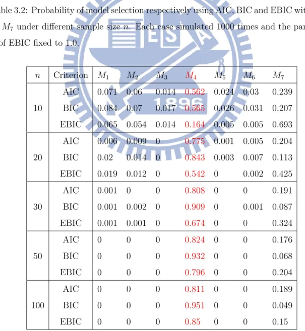
n is large enough (n ≥ 30), the performances of three information criterions are good,
and in this time, the result of BIC better than AIC is more significant than when n is not large enough. In addition, three information criterions indeed exist the large models tendency mentioned in Schwarz (1978) and Chen & Chen (2008). And no matter n is how much, the results of EBIC are worse than BIC, even worse than AIC in the case of
Table 3.1: AIC, BIC and EBIC values of one simulated data set (n = 100) of the true model M4 calculated under the original formula, approximative formula and function in
R. The original values of AIC, BIC and EBIC are calculated by the joint distribution of the sample x, (2.2.6) and (2.2.6) plus the the correction term, respectively. The approxi-mations are calculated by the formula for the three criterions.
Criterion Original Value Approximation function in R AIC 283.7878 281.1892 283.6349 BIC 286.8539 286.3996 294.0556 EBIC 289.0512 288.5968 296.2528
Table 3.2: Probability of model selection respectively using AIC, BIC and EBIC within M1
to M7 under different sample size n. Each case simulated 1000 times and the parameter
γ of EBIC fixed to 1.0. n Criterion M1 M2 M3 M4 M5 M6 M7 10 AIC 0.071 0.06 0.014 0.562 0.024 0.03 0.239 BIC 0.084 0.07 0.017 0.565 0.026 0.031 0.207 EBIC 0.065 0.054 0.014 0.164 0.005 0.005 0.693 20 AIC 0.006 0.009 0 0.775 0.001 0.005 0.204 BIC 0.02 0.014 0 0.843 0.003 0.007 0.113 EBIC 0.019 0.012 0 0.542 0 0.002 0.425 30 AIC 0.001 0 0 0.808 0 0 0.191 BIC 0.001 0.002 0 0.909 0 0.001 0.087 EBIC 0.001 0.001 0 0.674 0 0 0.324 50 AIC 0 0 0 0.824 0 0 0.176 BIC 0 0 0 0.932 0 0 0.068 EBIC 0 0 0 0.796 0 0 0.204 100 AIC 0 0 0 0.811 0 0 0.189 BIC 0 0 0 0.951 0 0 0.049 EBIC 0 0 0 0.85 0 0 0.15
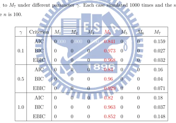
n = 10. Therefore, we compare information criterions under different γ, the parameter
involved in the correction term of EBIC, in the following.
Because γ only involve in the correction term of EBIC, it has nothing to do with AIC and BIC. So we only focus on comparing the impact of different γ on EBIC. In Table 3.3, the performance of EBIC is good but not better than BIC, and the larger γ, the worse
performan-ce of EBIC. Sinperforman-ce EBIC is applied suitably in the situation p greater than n, this result is expectable and acceptable.
Table 3.3: Probability of model selection respectively using AIC, BIC and EBIC within
M1 to M7 under different parameter γ. Each case simulated 1000 times and the sample
size n is 100. γ Criterion M1 M2 M3 M4 M5 M6 M7 0.1 AIC 0.000 0.000 0.000 0.841 0.000 0.000 0.159 BIC 0 0 0 0.973 0 0 0.027 EBIC 0 0 0 0.968 0 0 0.032 0.5 AIC 0 0 0 0.84 0 0 0.16 BIC 0 0 0 0.96 0 0 0.04 EBIC 0 0 0 0.929 0 0 0.071 1.0 AIC 0 0 0 0.82 0 0 0.18 BIC 0 0 0 0.963 0 0 0.037 EBIC 0 0 0 0.852 0 0 0.148 3.1.2 Autoregressive Model
Suppose that the true model is an AR(2) model with the paramters ϕ = (ϕ1, ϕ2) =
(0.6, 0.3), it can be written as
where ϵt is followed standard normal distribution. Given X0 = 0 and X1 = 0, and then
we generate the data of the model by above formula.
Table 3.4: Probability of model selection respectively using AIC, BIC and EBIC under different model sets. Each case simulated 1000 times and the sample size n is 100, the parameter γ of EBIC fixed to 1.0.
Max Order Criterion M1 M2 M3 M4 M5 M6 M7
2 AIC 0 0.01 0.99 BIC 0 0.158 0.842 EBIC 0 0.067 0.933 3 AIC 0 0.004 0.092 0.904 BIC 0 0.128 0.618 0.254 EBIC 0 0.086 0.183 0.731 4 AIC 0 0.003 0.02 0.079 0.898 BIC 0 0.127 0.539 0.185 0.149 EBIC 0 0.101 0.174 0.005 0.72 5 AIC 0 0 0.005 0.014 0.094 0.887 BIC 0 0.11 0.49 0.169 0.112 0.119 EBIC 0 0.134 0.186 0.021 0 0.659 6 AIC 0 0 0.002 0.008 0.019 0.092 0.879 BIC 0 0.107 0.502 0.127 0.109 0.068 0.087 EBIC 0.000 0.138 0.206 0.015 0.001 0 0.64
Consider the following models:
qquad M1 : Xt= ϵt qquad M2 : Xt= ϕ1Xt−1+ ϵt qquad M3 : Xt= ϕ1Xt−1+ ϕ2Xt−2+ ϵt (true) qquad M4 : Xt= ϕ1Xt−1+ ϕ2Xt−2+ ϕ3Xt−3+ ϵt qquad M5 : Xt= ϕ1Xt−1+ ϕ2Xt−2+ ϕ3Xt−3+ ϕ4Xt−4+ ϵt qquad M6 : Xt= ϕ1Xt−1+ ϕ2Xt−2+ ϕ3Xt−3+ ϕ4Xt−4+ ϕ5Xt−5+ ϵt
qquad M7 : Xt= ϕ1Xt−1+ ϕ2Xt−2+ ϕ3Xt−3+ ϕ4Xt−4+ ϕ5Xt−5+ ϕ6Xt−6+ ϵt,
and we use function in R to compute the value of AIC, BIC and EBIC, discovering which information criterion has the best performance.
In Table 3.4, since the maximum order of model is 2, (i.e. the true model has the maximum order in the model set,) the performance of AIC is the best, but if the max-imum order of model is larger than 2, the performance of AIC is the worst, and it has the maximum order tendency in the model sets. Therefore, we are unable to determine whether the best performance of AIC, when the maximum order equals 2, is based on the maximum order tendency or not. EBIC also has the same problem, maximum order tendency, but not so serious, better than AIC a little bit. Overall, BIC has the best performance, but not very good, when the order is greater than 3, only about half of the correct model selection rate.
3.1.3 Log-Normal Distribution vs. Exponential Distribution
Suppose we have a data set x = {x1, x2,· · · , xn}, which is generated from the
log-normal distribution ln N (0, 1). We want to use criterions to help us find the true dis-tribution. Since our problem is finding the true distribution, it is not involved in the models of different dimension, we only consider the comparison of models by AIC and BIC, regardless of EBIC.
Consider the following two models:
qquad M1 : Xi ∼ ln N(µ, σ2), i = 1, 2,· · · , n (true)
qquad M2 : Xi ∼ Exp(λ), i = 1, 2, · · · , n,
and we use the formulas of AIC and BIC to help us determine which model is true distri-bution.
For M1, the probability density function of a log-normal distribution is
fX(x|µ, σ2) = 1 xσ√2πexp{− (ln x− µ)2 2σ2 }, where µ = ln(E(X))− σ2 2 and σ 2 = ln(1 + V ar(X) [E(X)]2 )
. Let E(X) = ¯X and V ar(X) = s2
X,
then we use the estimators of µ, ˆµ = ln( ¯X)− σˆ2
2 , and σ 2, ˆσ2 = ln(1 + s2X ¯ X2 ) , to replace the parameters µ and σ2 respectively. For M
exponential distribution is
fX(x|λ) = λ exp{−λx}, x ≥ 0,
where λ = 1
E(X). Let E(X) = ¯X, then we have the estimator of λ, ˆλ =
1 ¯
X, and use it to
replace the parameter λ similarly.
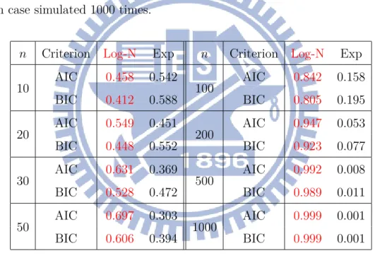
In Table 3.5, when n is not large enough, either AIC or BIC are only about half of the correct model selection rate. With n greater, the correct model selection rates of AIC and BIC will increase, and when n = 1000, the correct model selection rates of AIC and BIC are almost 1.
Table 3.5: Probability of model selection respectively using AIC and BIC within M1 and
M2. Each case simulated 1000 times.
n Criterion Log-N Exp n Criterion Log-N Exp
10 AIC 0.458 0.542 100 AIC 0.842 0.158 BIC 0.412 0.588 BIC 0.805 0.195 20 AIC 0.549 0.451 200 AIC 0.947 0.053 BIC 0.448 0.552 BIC 0.923 0.077 30 AIC 0.631 0.369 500 AIC 0.992 0.008 BIC 0.528 0.472 BIC 0.989 0.011 50 AIC 0.697 0.303 1000 AIC 0.999 0.001 BIC 0.606 0.394 BIC 0.999 0.001
3.2
High Dimensional Model (p > n)
Suppose there are p covariates X1, X2,· · · , Xp in a data, but the true model is Y = 1· X1+ 1· X2+ ϵ,
where Y = (Y1, Y2,· · · , Yn)T, Xi = (X1i, X2i,· · · , Xni)T, i = 1, 2,· · · , p and each
compo-nent of ϵ = (ϵ1, ϵ2,· · · , ϵn)T is normally distributed independent with mean 0 and variance
distribution.
Consider the following model sets:
qquad S1 ={Mj : Y = βjXj + ϵ, j = 1, 2,· · · , p}
qquad S2 ={Mj,r : Y = βjXj + βrXr+ ϵ, j, r = 1, 2,· · · , p, j ̸= r} (true)
qquad S3 ={Mj,r,s : Y = βjXj+ βrXr+ βsXs+ ϵ, j, r, s = 1, 2,· · · , p, j ̸= r ̸= s ̸= j},
and we compute the value of AIC, BIC and EBIC of each model in the above model sets, finding which model sets has the model of minimum value.
Table 3.6: Probability of model selection respectively using AIC, BIC and EBIC within
S1 to S3 and the status of model selection if given the model set S2 or S3. Each case
simulated 100 times and the sample size n is 30, the parameter γ of EBIC fixed to 1.0.
P Criterion S1 S2 S3 pr(MT|S2) pr(MT ⊂ MC|S3) 30 AIC 0 0 1 0 1 BIC 0 0.08 0.92 1 1 EBIC 0.04 0.71 0.25 1 1 35 AIC 0 0 1 0 1 BIC 0 0.04 0.96 1 1 EBIC 0.08 0.69 0.23 1 1 40 AIC 0 0 1 0 1 BIC 0 0 1 0 1 EBIC 0.08 0.72 0.2 1 1 45 AIC 0 0 1 0 1 BIC 0 0.04 0.96 1 1 EBIC 0.09 0.71 0.2 1 1 50 AIC 0 0 1 0 1 BIC 0 0.02 0.98 1 1 EBIC 0.12 0.64 0.24 0.969 1
In Table 3.6, the result of EBIC with respect to the AIC and BIC is pretty good; BIC only has less than one tenth correct rate, AIC completely tends to large model set
(the probability of S2 being chosen is 0). In addition, we further discuss the situation of
model selection if S2 or S3 being chosen. If S2 being chosen, then the rate of choosing
true model is greater than 96.9%; while in the case of S3 being chosen, the model which
be chosen must include the true covariates (X1 and X2), that is, the covariates of the
model is {X1, X2, X3}, {X1, X2, X4}, etc.
Table 3.7: Probability of model selection respectively using AIC, BIC and EBIC within
M1 to M5 under different model space p. Each case simulated 1000 times and the sample
size n is 100, the parameter γ of EBIC fixed to 1.0.
p Criterion M1 M2 M3 M4 M5 100 AIC 0.000 0.746 0.131 0.085 0.038 BIC 0 0.953 0.045 0.002 0 EBIC 0 0.998 0.002 0 0 200 AIC 0 0.764 0.12 0.077 0.039 BIC 0 0.962 0.035 0.003 0 EBIC 0 0.999 0.001 0 0 300 AIC 0 0.751 0.14 0.075 0.034 BIC 0 0.964 0.033 0.003 0 EBIC 0 1 0 0 0 400 AIC 0 0.749 0.136 0.078 0.037 BIC 0 0.958 0.039 0.003 0 EBIC 0 0.999 0.001 0 0 500 AIC 0 0.757 0.119 0.077 0.047 BIC 0 0.965 0.032 0.003 0 EBIC 0 1 0 0 0
Now we consider the similar situation with previous case n > p. Consider the fol-lowing models:
qquad M1 : Y = β1X1+ ϵ
qquad M3 : Y = β1X1+ β2X2+ β3X3+ ϵ
qquad M4 : Y = β1X1+ β2X2+ β3X3+ β4X4+ β5X5 + ϵ qquad M5 : Y = β1X1+ β2X2+· · · + β10X10+ ϵ,
and we compute the value of AIC, BIC and EBIC, finding which information criterion has the best performance.
In Table 3.7, even in the situation p greater than n (n = 100), AIC, BIC and EBIC still have very good performance, EBIC even achieve almost error-free result. This means that the additional correction term of EBIC, based on BIC, indeed can eliminate the large models tendency.
4
Conclusion
In the situation n greater than p, three information criterions mentioned in our study still have the large models tendency, especially when the data is generated from autore-gressive model. Inversely, in the situation p greater than n, it seems that we get a good solution when the data is generated from standard normal distribution. We maybe com-pare the data which is generated from other distributions, or furthermore, comparing and analyzing the real data in the future.
References
[1] Akaike, H. (1974), “A New Look at the Statistical Model Identification,” IEEE
Trans-actions on Automatic Control, 19, 716-723.
[2] Burnham, K. P. and Anderson, D. R. (2004), “Multimodel Inference: Understanding AIC and BIC in Model Selection,” Sociological Method & Research, 33, 261-304. [3] Chen, J. and Chen, Z. (2008), “Extended Bayesian information criteria for model
selection with large model spaces,” Biometrika, 95, 759-771.
[4] Edwards, D., Abreu, G. C. G. and Labouriau, R. (2010), “Selecting high-dimensional mixed graphical models using minimal AIC or BIC forests,” Edwards et al. BMC
Bioinformatics, 11:18.
[5] Konishi, S. and Kitagawa, G. (2008), Information Criteria and Statistical Modeling,
New York: Springer.
[6] Laplace, P. S. (1774), “Memoir on the probability of causes of events,” Laplace’s
Oeuvres complètes, 8, 27-65.
[7] Schwarz, G. (1978), “Estimating the Dimension of a Model,” The Annals of Statistics,
6, 461-464.
[8] Shumway, R. H. and Stoffer, D. S. (2011), Time Series Analysis and Its Applications: With R Examples, 3rd ed, New York: Springer.
[9] Wang, Y. and Liu, Q. (2006), “Comparison of Akaike information criterion (AIC) and Bayesian information criterion (BIC) in selection of stock-recruitment relationships,”