ANALYTIC-FUNCTIONS FOR ATOMIC MOMENTUM-DENSITY DISTRIBUTIONS AND COMPTON PROFILES OF K-SHELLS AND L-SHELLS

PHYSICAL REVIEWA VOLUME 47, NUMBER 5 MAY 1993

Analytic functions

for

atomic

momentum-density

distributions

and Compton

profiles

of

K

and

L

shells

Y.

F.

Chen and

C. M.

Kwei

Department

of

Electronics Engineering, National Chiao Tung Uniuersity, Hsinchu, Taiwan, Republic

of

China

C.

J.

Tung

Institute

_of

Nuclear Science, National Tsing Hua University, Hsinchu, Taiwan, Republic ofChina (Received 11 September 1992;revised manuscript received 29 December 1992)

An analytical expression involving three parameters was proposed for atomic momentum-density dis-tributions ofKand Lshells. This expression was based on the superposition ofhydrogenic closed-shell momentum densities. Parameters in the expression were determined by requiring four ofits moments to be equal to the corresponding Hartree-Fock results. An analytical function for the Cornpton profiles was then derived using the impulse approximation. Excellent agreement was found between the present results and detailed theoretical computations.

PACS number(s): 31.20.Sy,31.15.

+

q

I.

INTRODUCTION

II.

THEORY

The atomic electron-density distribution in momentum

space plays an important role in many applications.

For

instance, this distribution is directly related to Compton profiles, which represent the Doppler broadening

of

Compton lines due to moving electrons

[1].

Moreover,

this distribution is needed for the calculation

of

stopping

cross sections, shell corrections, and ionization cross sec-tions by the binary-encounter theory [2,

3].

Thus, a study

of

the momentum-density distribution isimportant.

In all these applications, a simple analytical function

for atomic momentum densities for each shell is desired. This function will help the manipulation

of

such densi-ties, usually calculated by the Hartree-Fock (HF)

ap-proach with data presented in tabulated form, in a very

simple way. Although an analytical expression for

momentum-space wave functions in the configurational Slater-type orbitals was reported [4] and hence an atomic

momentum-density distribution could be derived, this ex-pression involved too many terms and parameters to be

of

useful applications.

In this work, we propose a simple analytical form in-volving three parameters for atomic momentum-density distributions

of

K

and

L

shells. This form is based on the superposition

of

hydrogenic closed-shell momentum

den-sities. Parameters in the form are determined by

requir-ing the zeroth, first, second, and third moments

of

these distributions tobe equal to the corresponding

HF

results.

The hydrogenic model was previously applied to

calcu-late ionization-generalized oscillator strengths using the sum-rule constrained classical-binary-collision model

[5,

6].

The present work concerns the construction

of

analytical functions for the momentum-density distribu-tions and Compton profiles for each shell.

To

the best

of

our knowledge, no such function for Compton profiles is available except forthe helium atom

[7].

where

R„&(r)

is the radial part

of

P(r),

j

t(pr) is the

spheri-cal Bessel function, n is the principal quantum number, and l is the angular-momentum quantum number. The

momentum-density distribution for each shell can then be developed using

P„i(p).

The momentum-density distribution for a closed-shell hydrogenic atom is given by [8]

5 2

I(p)

=47tp p(p)

=

(g2+

2)4 (3)

where p(p) isthe normalized momentum-density

distribu-tion,

i.e.

,

f

47rp _p(p)dp

=1,

and _g

/2=E

is the average

kinetic energy

of

electrons in that shell. Note that atomic

units are used throughout this paper. Comparing the average kinetic energy

of

electrons,

i.

e., the second mo-ment

of

the momentum-density distribution, obtained us-ing Slater's rules [9] for the hydrogenic closed shell with corresponding

HF

data

[10],

we find that the error is within 2%%uo for the

K

shell and 6%%uo for the

L

shell for all

atoms. Toimprove the accuracy

of

Eq. (3),we propose

I,

(p)=47rp _p,

(p)=

.

g

2 .2 4 (i

=K,

L)

~,

=i

(0';,

+p')'

(4) The momentum-space atomic wave functions are defined as the Fourier transform

of

coordinate-space atomic wave functions,

i.e.

,

P(p)

=

1 7tr(r)exp(

—

ip

r)dr

. (27r)'~

In the central-field approximation, Eq. (1) reduces to

1/2

2

r

R„t(r)ji(pr

)dr,

0

47

BRIEF

REPORTS 4503

for the ith-she11 momentum-density distribution. Here we take A;J and g;J as parameters

to

be determined by re-quiring several moments

of

I,

(p)in

Eq.

(4)to be equal to

the corresponding

HF

results.

The mth moment

of

the ith-she11 momentum-density distribution is defined by

(p

);

=

f

"p

I;(p)dp

.

Letting m

=0,

1, 2, 3in Eqs. (4)and (5), we get

TABLE

I.

Parameters in Eq. (4)

density distribution of

E

shell. Element

{Z)

for atomic

momentum-CKI

TABLE

II.

Parameters in Eq. (4)

density distribution of

I.

shell.

for atomic

momentum-He (2) Li (3) Be (4) (5) C (6) N (7) O (8) (9) Ne (10) Na (11) Mg {12) Al (13) Si (14) P {15) S (16) Cl (17) Ar {18) K (19) Ca (20) Sc(21) Ti (22) V (23) Cr (24) Mn (25) Fe (26) Co (27) Ni (28) CU (29) Zn (30) Ga (31) Ge (32) As (33) Se (34) Br (35) Kr (36) Rb (37) Sr (38) Y (39) Zr (40) Nb (41) Mo (42) Tc (43) Ru (44) Rh (45) Pd (46) Ag (47) Cd (48) In (49) Sn (50) Sb (51) Te (52) (53) Xe (54) 0.8525 0.8849 0.9042 0.8989 0.8861 0.8685 0.8507 0.8240 0.7862 0.7603 0.7421 0.7283 0.7170 0.7099 0.7066 0.6702 0.6812 0.6676 0.6719 0.6855 0.6760 0.6134 0.6653 0.6479 0.6530 0.7137 0.6689 0.7009 0.6258 0.5767 O.S693 0.5767 0.6294 0.6428 0.5949 0.4484 0.4599 0.4491 0.4464 0.4450 0.4420 0.4248 0.4444 0.4359 0.4233 0.4441 0.4537 0.5085 0.4326 0.4261 0.4216 0.4325 0.4053 1.4913 2.4761 3.4634 4.4190 5.3588 6.2866 7.2103 8.1134 8.9904 9.8862 10.795 11.711 12.632 13.540 14.501 15.360 16.332 17.246 18.208 19.202 20.130 20.891 22.018 22.919 23.895 25.063 25.877 26.952 27.637 28.413 29.337 30.330 31.508 32.526 33.283 33.519 34.540 35.427 36.360 37.303 38.237 39.082 40.163 41.061 41.922 43.029 44.037 45.348 45.810 46.721 47.640 48.683 49.418 2.5586 3.9533 5.3326 6.5313 7.6444 8.7043 9.7528 10.731 11.644 12.630 13.651 14.690 15.736 16.751 17.878 18.766 19.917 20.922 22.028 23.188 24.205 24.915 26.275 27.235 28.332 29.843 30.565 31.879 32.409 33.156 34.167 35.255 36.645 37.796 38~522 38.749 39.839 40.823 41.846 42.873 43.892 44.833 45.969 46.956 47.925 49.063 50.158 51.514 52.096 53.089 54.096 55.185 56.064 Element (Z) Li (3) Be (4) B (5) C (6) N (7) O (8)

F

(9) Ne (10) Na (11) Mg (12) Al (13) Si (14) P (15) S (16) Cl (17) Ar (18) K (19) Ca (20) Sc (21) Ti (22) V (23) Cr (24) Mn (25) Fe (26) Co (27) Ni (28) Cu {29) Zn (30) Ga (31) Ge (32) As (33) Se (34) Br {35) Kr (36) Rb (37) Sr (38) Y (39) Zr (40) Nb (41) Mo (42) Tc (43) Ru (44) Rh (45) Pd (46) Ag (47) Cd (48) In (49) Sn (50) Sb (51) Te (52}

I

(53) Xe (S4) 0.9590 0.9397 0.9404 0.9414 0.9429 0.9421 0.9411 0.9401 0.9447 0.9482 0.9512 0.9534 0.9552 0.9565 0.9572 0.9589 0.9599 0.9621 0.9611 0.9609 0.9606 0.9602 0.9599 0.9623 0.9591 0.9588 0.9589 0.9568 0.9564 0.9561 0.9554 0.9552 0.9540 0.9546 0.9548 0.9556 0.9546 0.9546 0.9544 0.9544 0.9541 0.9543 0.9543 0.9544 0.9541 0.9548 0.9542 0.9547 0.9546 0.9547 0.9548 0.9548 CL1 0.3994 0.5648 0.9017 1.2426 1.5831 1.8881 2.2003 2.5174 3.0233 3.5191 4.0133 4.5025 4.9895 5.4715 5.9499 6.4371 6.9192 7.4138 7.8835 8.3592 8.8346 9.3077 9.7816 10.283 10.724 11.192 11.675 12.128 12.597 13.067 13.536 14.007 14.473 14.951 15.427 15.911 16.377 16.854 17.328 17.806 18.281 18.760 19.238 19.718 20.194 20.678 21.153 21.637 22. 116 22.597 23.079 23.561 1.2 2.5381 3.4130 4.1177 4.7817 5.4258 6.0270 6.5902 7.1266 8.0953 9.0622 10.023 10.958 11.884 12.778 13.638 14.573 15.457 16.458 17.167 17.933 18.694 19.435 20.181 21.878 21.647 22.289 23.142 23.665 24.379 25.088 25.758 26.461 27.033 27.860 28.629 29.487 30.060 30.783 31.473 32.200 32.868 33.619 34.331 35.054 35.718 36.534 37.127 37.921 38.605 39.324 40.036 40.746

4504 BRIEFREPORTS 47 2

3;

g;

=a

(p

);

(m

=0,

1, 2,

3),

j=1

(6) 0..5 I I I I I I I I I I I I I I I I I I I I I I I 1

I;(p)

J;(q)

=

f

dp,

2 q p (7) where

a0=1,

a&

=3m/8,

a2=1,

and

a3=3~/16.

This

procedure guarantees the zeroth, first, second, and third moments

of

Eq. (4) to be equal to those

of

the

HF

momentum-density distribution. Note that the zeroth moment in Eq. (6)is simply the normalization condition,

i.

e.

,

3;&+A,

2=1.

This condition leaves the number

of

free parameters in

Eq.

(4)equal to three. The simultane-ous equations

of Eq.

(6)can be solved for A;~ and g;.

us-ing

HF

data for

_(p

);.

Applying

HF

data for available atoms with

Z

up to 54

[10],

we have solved these equa-tions for the ground-state

X

and

L

shells. Solutions are given in Tables

I

and

II.

Under the impulse approximation

[11],

the isotropic

Compton profile

of

the ith shell,

_J,

._{(q), is related}

_to

_the momentum-density distribution as

p4

0.3

02

0.1 0.0 0 10 15 p

(a.

u.

)

20 25

where Z, isthe occupation number

of

electrons per atom in the ith shell and _{q is}the projection

of

electron momen-tum before the collision on the direction

of

momentum

transfer. Substituting Eq. (4) into Eq. (7), we find the

analytical expression forCompton profiles as 8Z,

J;(q)=

_g

(i

=K,

l.

)

.

3

~

(f2~~

+

_q 2 )3

III.

RESULTS

Using

Eq.

(4) with parameters listed in Tables

I

and

II,

we have calculated atomic momentum-density distribu-tions

of

K

and

L

shells. Figure 1 shows a comparison

of

0..20 I I I 1

( I I I t

I I I I ~

I I I I I

I I I I I

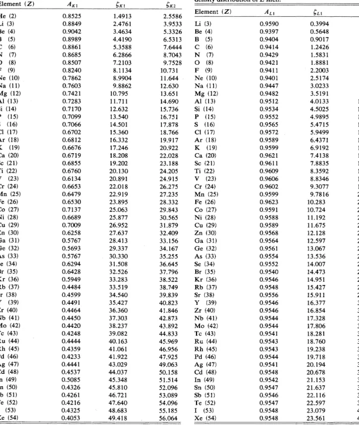
FIG.

2. Plot ofthe L-shell electron momentum-density distri-bution for several atoms. Present results (solid curves) are com-pared toHFdata (dashed curves) [10].Atomic units are used.

our results with the corresponding

HF

data

[10]

forthe

K

shell

of

several atoms. Excellent agreement is found for

all atoms. The present results (solid curves) and the

HF

data (dashed curves, but merging into solid curves within graphic scales) agree so closely with each other that one cannot see any difference from the figure. A similar plot

for the

L

shell is shown in Fig.

2.

Again, the agreement isso close that only minute differences can be seen.

Fig-p4

0.3 ell 0.15 0.2

0.

10 C4 0.1 0.05 0.0 0 10 20 Z 30 40 50 0.00 0 10 20 30 p

(a.

u.

)

40 50

FIG.

1.. Plot ofthe K-shell electron momentum-density

dis-tribution for several atoms. Present results (solid curves) are compared to HFdata (dashed curves, but coinciding with solid curves within graphic scales) [10].Atomic units are used.

FIG.

3. Plot ofthe E-shell Compton profile as a function of atomic number for three momentum values. Present results (solid circles) are compared to data calculated using HF wave functions (open circles, but coinciding with solid circles within graphic scales) [12].The curves are interpolating results show-ing the dependence ofthe Compton profile on atomic number. Atomic units are used.

47

BRIEF

REPORTS 4505

3.

0

2.5

2.

0—

hell

merging into solid circles within graphic scales)

[12].

Note that all calculated results are plotted as discrete

points; interpolating curves serve only to indicate the dependence

of

these results on atomic number. A similar plot

of

the L-shell Compton profile is shown in

Fig. 4.

Still, only minute differences can be seen.

1.

5

1.

0

0.

5

0.0

0 10 20 30 40 50

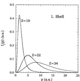
FIG.

4. Plot ofthe L-shell Compton profile as a function of atomic number for three momentum values. Present results (solid circles) are compared to data calculated using HF wave functions (open circles) [12]. The curves are interpolating re-sults showing the dependence ofthe Compton profile on atomic number. Atomic units are used.

IV. CONCLUSION

In this work, we have constructed simple analytical

ex-pressions for the atomic momentum-density distribution and Compton profile

of

E

and

L

shells. Although it was

not discussed, we have calculated the stopping cross

sec-tion

of

IC and

L

shells for protons using Eq. (4) and the stopping-power formula

[13].

In all these calculations, we found excellent agreement between the present results and detailed theoretical computations.

An extension

of

this work to other shells seems

plausi-ble. Ekowever, the superposition

of

hydrogenic closed-shell momentum densities in

Eq.

(4) should include more

terms.

It

requires then additional moments in

Eq.

(5)to

be applied.

If

electrons in the

M

and higher shells belong

to the valence band, a solid-state rather than atomic

theory must be employed.

ure 3 is a plot

of

the X-shell Compton profile as a

func-tion

of

atomic number for several momentum values. No

difference can be seen from the figure between the present results (solid circles) and the

HF

data (open circles, but

ACKNOWLEDGMENT

This research was supported by the National Science

Council

of

the Republic

of

China.

[1]

B.

G. Williams, Compton Scattering (McGraw-Hill, New York, 1977).

[2]

J.

H. McGuire and

K.

Omidvar, Phys. Rev. A 10, 182 (1974).

[3]

J.

R.

Sabin and

J.

Oddershede, Phys. Rev. A 26, 3209 (1982).

[4]

F. F.

Komarov and M. M. Temkin,

J.

Phys. B9, L255 (1976).

[5]C.

J.

Tung, Phys. Rev. A 22,2550 (1980).

[6] C. M.Kwei, Y.

F.

Chen, and C.

J.

Tung, Phys. Rev.A 45, 4421(1992).

[7]

T.

Kogaand H.Matsuyama, Phys. Rev.A45,5266(1992). [8] V. Fock, Z.Phys. 98,145(1935).

[9]

B. B.

Robinson, Phys. Rev. 140, A764 (1965).

[10]

E.

Clementi and C. Roetti, At. Data Nucl. Data Tables 14, 177(1974).

[11]L.Mendelsohn and V. H. Smith, in Compton Scattering, edited by

B. G.

Williams (McGraw-Hill, New York, 1977), p. 102.

[12]

F.

Biggs, L.

B.

Mendelsohn, and

J. B.

Mann, At. Data Nucl. Data Tables 16,201(1975).