Numerically Stable, Structure-preserving Algorithms for
Palindromic Quadratic Eigenvalue Problems
Jiang Qian∗ Tsung-Min Hwang† Wen-Wei Lin‡
Abstract
In this paper, we first write the palindromic quadratic eigenvalue problem as a >-symplectic pencil which preserves the reciprocity property of the eigenvalues. Then we develop numerically stable, structure-preserving algorithms to solve the >-symplectic pen-cil by using the (S +S−1)-transformation and H2-transformation, respectively. Numerical
experiments show that the numerical approach by (S + S−1)-transformation applied to the finite element model of the high-speed trains and rails performs better than the ap-proach by H2-transformation and QZ algorithm, because it preserves the >-symplectic
structure without using the Cayley transformation.
Key words. palindromic eigenvalue problem, >-Hamiltonian pencil, >-symplectic pen-cil
1
Introduction
We consider the palindromic quadratic eigenvalue problem (QEP)
P (λ)x ≡ (λ2A>1 + λA0+ A1)x = 0, (1.1)
where A1, A0 ∈ Cn×n, and A>0 = A0. Here and throughout this paper A> denotes the
transpose (not conjugate transpose) of a matrix A. Such a QEP arises in the vibration analysis of fast trains, as indicated by the amount of publicity given to the palindromic QEP
[8]. The coefficient matrices A0 and A1 in (1.1) depend on some parameter ω associated
with the excitation frequency of the external force. This problem is known as a palindromic
QEP since A1 appears at both ends of (1.1) and A0 is symmetric. Consequently, by taking
∗School of Sciences, Beijing University of Posts and Telecommunications, Beijing, 100876, China;
Depart-ment of Mathematics, National Tsinghua University, Hsinchu, 300, Taiwan (jqian104@ gmail.com). This author’s research was partly supported by Project NSFC 10571007.
†Department of Mathematics, National Taiwan Normal University, Taipei, 116, Taiwan
‡Department of Mathematics, National Tsing Hua University, Hsinchu, 300, Taiwan
the transpose of (1.1), we can easily see that the eigenvalues of (1.1) have a ‘symplectic’ property, that is, they are symmetrically placed with respect to the unit circle, containing both an eigenvalue λ and its reciprocal 1/λ.
Practically, to optimize the design of the rail and the train, all 2n eigenvalues and their associated eigenvectors are desired. A standard approach of finding all eigenpairs is to work with a 2n × 2n linearized form and compute its generalized Schur form (see [17]). However, the symplectic structure in (1.1) is not preserved by the linearizations, generally, producing large numerical errors ([8]). Recently, some pioneer work [6, 12, 11] discovered that the
palindromic QEP (1.1) could be linearized in the form λZ ±Z>, which preserves symplecticity
to some extent, and suggested a structure-preserving method to solve the linearized eigenvalue problem. This does lead to a vast improvement over previous approaches, but some numerical results seem not accurate enough, and the numerical algorithm is still under development. Chu et al [2] proposed a structure-preserving doubling algorithm for the computation of a solvent of a nonlinear matrix equation associated with the palindromic QEP. The numerical results show much promise, but the basic tools and the convergence theory are incomplete.
As mentioned before, the linearizations, generally, cannot preserve the symplectic struc-ture in (1.1). Fortunately, with the special linearization
(M − λL)z ≡ µ· A1 0 −A0 −I ¸ − λ · 0 I A>1 0 ¸¶ · x y ¸ = 0, (1.2)
the symplectic structure of eigenpairs is preserved. Actually, it can be easily verified that M and L satisfy
MJ M>= LJ L>, (1.3)
where J is the 2n × 2n matrix ·
0 In
−In 0
¸
with In being the n × n identity matrix. In this
paper, we are to propose two numerically stable, structure-preserving algorithms to compute all eigenvalues and associated eigenvectors of the matrix pencil M − λL. It is easily seen
that if (λ, [x> y>]>) is an eigenpair of the pencil M − λL, then (λ, x) is an eigenpair of the
palindromic QEP (1.1).
When M and L in (1.3) are real matrices, the pencil M − λL is called a symplectic pencil. The problem of finding the eigenvalues of the symplectic pencil as well as the invariant subspace corresponding to the stable eigenvalues is closely related to obtaining a stabilizing solution of the discrete-time algebraic Riccati equation (DARE) [15]. Lin [10] proposed
a structure-preserving (S + S−1)- transformation for the computation of eigenvalues of the
symplectic pencil. However, non-orthogonal transformations are used in the method which in certain cases can cause numerical instability. Patel [16] improved Lin’s method and developed a numerically stable and reliable algorithm for reducing the pencil to a block triangular condensed form by using only orthogonal transformations.
An analogous problem is to find the eigenvalues of a Hamiltonian matrix or a Hamiltonian pencil, which arises in solving the continuous-time algebraic Riccati equation (CARE). Some
early works can be found in [9, 14]. By using the H2 transformation, Van Loan [18] proposed
a square reduced method relying on orthogonal symplectic similarity transformations which preserves the Hamiltonian structure and has desirable numerical properties. However, the
method may suffer from a loss of accuracy of order √², where ² is the machine precision.
Benner et al [1] developed a numerically stable, structure-preserving method using a URV-approach for the computation of eigenvalues of real Hamiltonian or symplectic pencils, which computes the eigenvalues to full possible accuracy. Recently, Chu et al [3] derived a new method for computing the Hamiltonian Schur form of a Hamiltonian matrix that has no purely imaginary eigenvalues, which is numerical strongly backward stable.
However, all these procedures cannot be applied to complex symplectic or Hamiltonian pencils and matrices (see [1, 18] for more details). In this paper, we extend Patel’s and Benner et al’s approaches to the pencil (1.2) resulting from the palindromic QEP (1.1). Only unitary transformations are used, and the symplectic structure is fully preserved in our approaches, which make the algorithms numerical stable and efficient.
The paper is organized as follows. In Section 2 we introduce notations and propose some basic results. Two structure-preserving numerical approaches are presented in Section 3 and 4, respectively. We illustrate numerical behaviors of algorithms by some examples from finite element models of fast trains [2] in Section 5. Conclusions are finally given in Section 6.
2
Preliminaries
In this section we give some basic definitions and preliminary results. We first introduce the classes of matrix pencils and matrices that are discussed in this paper.
Definition 2.1. (i) A pencil M − λL ∈ C2n×2n is >-symplectic, if MJ M>= LJ L>.
(ii) A pencil K − λN ∈ C2n×2n is >-Hamiltonian, if KJ N>= −N J K>.
(iii) A matrix H ∈ C2n×2n is >-Hamiltonian, if (HJ )>= HJ .
(iv) A matrix S ∈ C2n×2n is >-skew-Hamiltonian, if (SJ )>= −SJ .
(v) A matrix U ∈ C2n×2n is unitary >-symplectic, if UUH = I
2n and UJ U>= J . The set
of unitary >-symplectic matrices in C2n×2n is denoted by UTS2n. Here UH denotes the
conjugate transpose of U.
For simplicity, in this paper we only consider regular pencils. A pencil M − λL is called regular if det(M − λL) does not vanish identically for all complex numbers λ. Note that pencils and matrices defined in Definition 2.1 are different from the usual symplectic or Hamiltonian pencils and matrices. We use the transpose, instead of the conjugate transpose, of complex matrices in these definitions, except for the unitary >-symplectic matrix.
Similar to the well-known properties of real symplectic and Hamiltonian pencils [1], the following properties of >-symplectic and >-Hamiltonian pencils can be easily verified.
Proposition 2.1. (i) For a >-symplectic pencil M − λL, if ν is an eigenvalue of M − λL, so is 1/ν. This includes the zero eigenvalue with infinite eigenvalue as counterpart. (ii) For a >-Hamiltonian pencil K − λN , if µ is a finite eigenvalue of the pencil, so is −µ.
The next proposition gives the relationship between >-symplectic and >-Hamiltonian pencils.
Proposition 2.2. (i) Let M − λL be a >-symplectic pencil, and let γ = 1 or −1. Then
K − λN := (M − γL) − λ(γM + L) is >-Hamiltonian.
(ii) Let K − λN be a >-Hamiltonian pencil, and let γ = 1 or −1. Then M − λL :=
(γN + K) − λ(N − γK) is >-symplectic.
Proof. From (i) and (ii) of Definition 2.1 follows the proposition immediately.
The following proposition describes the special form and the property of a unitary >-symplectic matrix.
Proposition 2.3. (i) Any matrix U ∈ UTS2n is of the form U =
·
U1 U¯2
−U2 U¯1
¸
, where U1, U2 ∈ Cn×n, and ¯U denotes the complex conjugate of the matrix U .
(ii) For any matrix U ∈ UTS2n, if S is >-skew-Hamiltonian, then UHSU is still
>-skew-Hamiltonian.
Proof. (i) The fact that U is unitary and UJ U> = J give
UJ = J ¯U. (2.1) Partitioning U as U = · U1 U3 −U2 U4 ¸
, where Ui ∈ Cn×n, i = 1, . . . , 4 and comparing both
sides of (2.1), we easily obtain U3= ¯U2 and U4 = ¯U1.
(ii) Direct calculation gives
(UHSUJ )>= J>U>S>U = J U¯ >J SJ ¯U = −UHSUJ .
The second equality uses the fact S> = −J SJ , which is derived from the definition
of the >-skew-Hamiltonian matrix. The last equality uses the fact J U>J = −UH and
There are three types of unitary >-symplectic matrices which are of great importance in our numerical approaches. The first two types of unitary >-symplectic matrices are based on
Givens rotations. A standard Givens rotation in C2n×2n is given by
G(i, j, c, s) = Ii−1 c ¯s Ij−i−1 −s ¯c I2n−j , (2.2)
where c¯c + s¯s = 1. The first type of unitary >-symplectic matrices is of the form
Gs1(i, c, s) := G(i, n + i, c, s). (2.3)
The second type of unitary >-symplectic matrices is of the form
Gs2(i, j, c, s) := · G(i, j, c, s) 0 0 G(i, j, c, s)¯ ¸ . (2.4)
Here G(i, j, c, s) is an n × n Givens rotation. The third type of unitary >-symplectic matrices is based on the standard Householder transformation, and has the form
Hs(k, v) := · H(k, v) 0 0 H(k, v)¯ ¸ , (2.5) where H(k, v) = Ik⊕ (In−k − 2vvH
vHv) with v ∈ Cn−k. In the following two sections, we will
propose two numerical algorithms to find all eigenvalues and the associated eigenvectors of the >-symplectic pencil M − λL (1.2) by using unitary transformations whenever possible and hence are numerically stable.
3
Numerical Approach I
The first algorithm is developed based on Patel’s approach in [16] applying to the (S + S−1
)-transformation of a real symplectic pencil [10] for the computation of all eigenvalues. In this section, we will extend Patel’s approach to >-symplectic pencils, and propose an algorithm to compute all eigenvalues and the associated eigenvectors of the >-symplectic pencil (1.2).
Theorem 3.1 gives the relationship between eigenvalues and eigenvectors of a >-symplectic
pencil and those of its (S + S−1)-transformation.
Theorem 3.1. Let M − λL be a >-symplectic pencil, and let ˆM − λ ˆL be its (S + S−1
)-transformation, that is,
ˆ
M ≡ MJ L>+ LJ M>, L ≡ LJ Lˆ >. (3.1)
(i) µ is a double eigenvalue of ˆM − λ ˆL if and only if ν,1
ν are eigenvalues of M − λL, where
ν,1ν are two roots of the quadratic equation λ +λ1 = µ.
(ii) Let x and y be the eigenvectors of L>−λM>corresponding to ν and ν1, respectively, i.e.,
(L>− νM>)x = 0 and (L>−1
νM>)y = 0. Then x and y are two linearly independent
eigenvectors of ˆM − λ ˆL corresponding to µ = ν +ν1.
(iii) Furthermore, from (ii) if z = αx + βy with αβ 6= 0 is an eigenvector of ˆM − λ ˆL corresponding to µ = ν +1ν(µ 6= ±2), i.e., ( ˆM − µ ˆL)z = 0, then J (L>−1
νM>)z and
J (L>− νM>)z are the eigenvectors of M − λL corresponding to ν and 1
ν, respectively.
Proof. (i) Since M − λL is >-symplectic, i.e., MJ M>= LJ L>, by (3.1) it holds
ˆ M − µ ˆL = MJ L>+ LJ M>− (ν + 1 ν)LJ L > = (M − νL)J (L>− 1 νM >) = (M − 1 νL)J (L >− νM>). (3.2)
Hence (i) follows obviously.
(ii) From the last two equations of (3.2) follows that ( ˆM − µ ˆL)x = (M − 1 νL)J (L >− νM>)x = 0, and ( ˆM − µ ˆL)y = (M − νL)J (L>−1 νM >)y = 0. (iii) Since ν 6= 1
ν, x and y should be linearly independent. By applying the last two equations
of (3.2) again, it only remains to show that J (L>−ν1M>)z 6= 0 and J (L>− νM>)z 6=
0. From (ii) we have
J (L>− 1 νM >)z = J (L>− 1 νM >)(αx + βy) = αJ (L>−1 νM >)x 6= 0. Similarly, J (L>− νM>)z = J (L>− νM>)(αx + βy) = βJ (L>− νM>)y 6= 0.
Note that from (1.2) we have ˆ M − λ ˆL = MJ L>+ LJ M>− λLJ L> = · A1− A> 1 A0 −A0 A1− A>1 ¸ − λ · 0 −A1 A> 1 0 ¸ = µ· A0 A>1 − A1 A1− A> 1 A0 ¸ − λ · −A1 0 0 −A> 1 ¸¶ J . (3.3)
This implies that the pencil ˆM − λ ˆL has the same eigenvalues as the pencil K − λN , where
K = · A0 A>1 − A1 A1− A>1 A0 ¸ , N = · −A1 0 0 −A> 1 ¸ . (3.4)
Furthermore, if z is an eigenvector of K −λN corresponding to the eigenvalue µ, then ˆz = J z
is the eigenvector of ˆM − λ ˆL corresponding to the same µ.
It is easily seen that K and N in (3.4) are both >-skew-Hamiltonian. We now introduce two types of transformations that preserve this structure. The first type involves similarity
transformations on K and N using Givens >-symplectic matrices Gs1(i, c, s) defined in (2.3),
i.e.,
K := GHs1KGs1, N := GHs1N Gs1. (3.5)
It follows from Proposition 2.3 that the resulting K and N are still >-skew-Hamiltonian. The second type of transformations are of the forms:
K := QKZ, N := QN Z, (3.6) where Q = · U 0 0 V ¸ , Z = · V> 0 0 U> ¸ , (3.7)
with U, V ∈ Cn×n are unitary matrices representing the application of Givens rotations. One
can verify that K and N in (3.6) are still >-skew-Hamiltonian.
With these two types of transformations, we may now reduce K−λN to a block triangular structure, that is,
K := ˜QK ˜Z = · K11 K12 0 K11> ¸ , N := ˜QN ˜Z = · N11 N12 0 N11> ¸ , (3.8)
where K11 ∈ Cn×n is upper Hessenberg, N
11 ∈ Cn×n is upper triangular, and ˜Q, ˜Z are
unitary which are products of sequences of transformations mentioned above. This procedure is based on Patel’s approach [16], except that the orthogonal transformations are replaced by the unitary transformations as in (3.5) and (3.6). A pseudocode for this block triangular
reduction is provided in Appendix A.1, and a sketch of reductions (n = 4) is shown as follows, where the numbers above the arrow refer to corresponding lines of the pseudocode in Appendix A.1. K = × × × × 0 × × × × × × × × 0 × × × × × × × × 0 × × × × × × × × 0 0 × × × × × × × × 0 × × × × × × × × 0 × × × × × × × × 0 × × × × 01−05−→ × × × × 0 × × × × × × × × 0 × × × × × × × × 0 × × × × × × × × 0 0 × × × × × × × × 0 × × × × × × × × 0 × × × × × × × × 0 × × × × 07−24 −→ × × × × 0 × × × × × × × × 0 × × × × × × × × 0 × × × × × × × × 0 0 0 0 × × × × × 0 0 × × × × × × 0 × 0 × × × × × × × × 0 × × × × 25−32 −→ × × × × 0 × × × × × × × × 0 × × × × × × × × 0 × × × × × × × × 0 0 0 0 0 × × × × 0 0 × × × × × × 0 × 0 × × × × × 0 × × 0 × × × × 33−50 −→ × × × × 0 × × × × × × × × 0 × × 0 × × × × × 0 × 0 × × × × × × 0 0 0 0 0 × × 0 0 0 0 × × × × × × 0 × 0 × × × × × 0 × × 0 × × × × → · · · → × × × × 0 × × × × × × × × 0 × × 0 × × × × × 0 × 0 0 × × × × × 0 0 0 0 0 × × 0 0 0 0 0 0 × × × 0 0 0 0 0 × × × × 0 0 0 0 × × × ×
N = × × × × 0 0 0 0 × × × × 0 0 0 0 × × × × 0 0 0 0 × × × × 0 0 0 0 0 0 0 0 × × × × 0 0 0 0 × × × × 0 0 0 0 × × × × 0 0 0 0 × × × × 01−05 −→ × × × × 0 0 0 0 0 × × × 0 0 0 0 0 0 × × 0 0 0 0 0 0 0 × 0 0 0 0 0 0 0 0 × 0 0 0 0 0 0 0 × × 0 0 0 0 0 0 × × × 0 0 0 0 0 × × × × 07−24−→ × × × × 0 0 0 0 0 × × × 0 0 0 0 0 ⊗ × × 0 0 0 0 0 0 ⊗ × 0 0 0 0 0 0 0 0 × 0 0 0 0 0 0 0 × × ⊗ 0 0 0 0 0 × × × ⊗ 0 0 0 0 × × × × 25−32−→ × × × × 0 0 0 × 0 × × × 0 0 0 × 0 0 × × 0 0 0 × 0 0 0 × × × × 0 0 0 0 0 × 0 0 0 0 0 0 0 × × 0 0 0 0 0 0 × × × 0 0 0 0 0 × × × × 33−50−→ × × × × 0 × × × 0 × × × × 0 × × 0 ⊗ × × × × 0 × 0 0 ⊗ × × × × 0 0 0 0 0 × 0 0 0 0 0 0 0 × × ⊗ 0 0 0 0 0 × × × ⊗ 0 0 0 0 × × × × → · · · → × × × × 0 × × × 0 × × × × 0 × × 0 0 × × × × 0 × 0 0 0 × × × × 0 0 0 0 0 × 0 0 0 0 0 0 0 × × 0 0 0 0 0 0 × × × 0 0 0 0 0 × × × ×
From (3.8), we can see that the pencil K11−λN11contains half of eigenvalues of the pencil
K−λN , and K>
11−λN11> contains the other half which is exactly the same as those eigenvalues
of K11− λN11. We then apply QZ algorithm to the pencil K11− λN11 for computing all
eigenpairs {(µi, yi)}ni=1. Consequently, {(µi, zi(≡ ˜Z
·
yi
0 ¸
))}n
i=1 are n eigenpairs of K − λN .
From (3.3) it follows that {(µi, xi(= J zi))}n
i=1are eigenpairs of ˆM−λ ˆL. Finally, We compute
all eigenvalues and the associated eigenvectors of M − λL by (iii) of Theorem 3.1. Algorithm 3.1.
Input : A >-symplectic pencil M − λL ∈ C2n×2n of the form (1.2).
Output : All eigenvalues and eigenvectors of M − λL. Step 1. Form the pencil K − λN as in (3.4);
Step 2. Reduce K − λN to block upper triangular forms in (3.8) using unitary transforma-tions as in (3.5) and (3.6). (See a pseudocode in Appendix A.1);
Step 3. Use QZ algorithm to compute eigenpairs {(µi, yi)}ni=1of K11−λN11defined in (3.8);
Step 4. Compute ˆzi = J ˜Z · yi 0 ¸ , i = 1, 2, . . . , n;
Step 5. Compute eigenvalues νi and ν1i of M − λL by solving the quadratic equations ν2−
µiν + 1 = 0; Compute eigenvectors J (L>−ν1iM>)ˆzi, J (L>− νiM>)ˆzi corresponding
to νi,ν1i, respectively, for i = 1, 2, . . . , n.
Remark 3.1 (i) In Step 2, since both eigenvalues and eigenvectors are required, the
transformation matrix ˜Z in (3.8) needs to be accumulated, while ˜Q does not need to be
constructed explicitly.
(ii) In Step 3, since K11− λN11 is already in a Hessenberg-triangular form, the first step
in QZ algorithm which is the reduction to such a form is not needed.
(iii) In Step 5, when νi is too large, special care should be taken to avoid big roundoff
error while solving the quadratic equation.
(iv) In Step 5, if the norm of J (L>−ν1iM>)ˆzi or J (L>− νiM>)ˆzi is small, we use one
step inverse iteration to compute an approximate eigenvector.
(v) The algorithm needs approximately 27n3 flops for eigenvalues, and additional 23n3
flops for eigenvectors (exclude inverse iteration modifications). While QZ algorithm applied
directly to the pencil M − λL needs approximately 120n3flops for eigenvalues and additional
260
3 n3 flops for eigenvectors. Here and hereafter a flop is a floating point multiplication for
complex numbers, which involves 6 real flops.
4
Numerical Approach II
Benner, Mehrmann and Xu [1] proposed a numerically stable, structure preserving algorithm, say URV-approach, for finding all eigenvalues of real Hamiltonian pencils. As for real sym-plectic pencils, the Cayley transformations are first applied to transform into Hamiltonian pencils, and then the algorithm is applied. In this section, we are to extend this algorithm to solving the >-symplectic pencil M − λL (1.2). From Proposition 2.2 follows that if γ = 1 or −1, then
K − λN := (M − γL) − λ(γM + L) (4.1)
is a >-Hamiltonian pencil. It is easily seen that the pair (νi, xi) is an eigenpair of K − λN if
Theorem 4.1. Let K −λN be a >-Hamiltonian pencil and ˆK −λ ˆN be its H2-transformation,
i.e.,
ˆ
K := KJ K>, N := N Jˆ >N>. (4.2)
Then
(i) µ is a double eigenvalue of ˆK − λ ˆN if and only if ±√µ are eigenvalues of K − λN . (ii) Let x and y be the eigenvectors of K>− λN> corresponding to√µ and −√µ,
respec-tively, i.e., (K>−√µN>)x = 0 and (K>+√µN>)y = 0. Then x and y are two linearly
independent eigenvectors of ˆK − λ ˆN corresponding to µ.
(iii) Furthermore, from (ii) if z = αx + βy with αβ 6= 0 is an eigenvector of ˆK − λ ˆN corresponding to µ (µ 6= 0), i.e., ( ˆK − µ ˆN )z = 0, then J (K>−√µN>)z and J (K>+
√
µN>)z are the eigenvectors of ˆK − λ ˆN corresponding to √µ and −√µ, respectively.
Proof. Since K − λN is >-Hamiltonian, i.e., KJ N>= −N J K>, by (4.2) it holds
ˆ
K − µ ˆN = KJ K>− µN J>N>
= (K −√µN )J (K>−√µN>)
= (K +õN )J (K>+õN>).
The theorem follows by using the same argument as in the proof of Theorem 3.1.
For computing eigenvalues and eigenvectors of the pencil ˆK − λ ˆN , we first reduce K
and N to a condense form. We compute unitary Q ∈ C2n×2n and unitary >-symplectic
U, V ∈ UTS2n such that
QKU = · K11 K12 0 K22 ¸ , QN V = · N11 N12 0 N22 ¸ , (4.3)
where K11, N11, K22> ∈ Cn×n are upper triangular, and N22> is upper Hessenberg. Such a
reduction can be obtained via a finite-step elimination procedure, based on Algorithm 4.3 (URV-approach) in [1], except that the orthogonal symplectic transformations are replaced by three types of unitary >-symplectic transformations defined in (2.3)-(2.5). For the details of the reduction, we refer the readers to [1]. A pseudocode for such reduction can be found in Appendix A.2.
Note that U, V in (4.3) are unitary >-symplectic, which implies that U J U> = J and
V J V>= J . Hence, we have QKJ K>Q>J = QKU J U>K>Q>J = · K11 K12 0 K22 ¸ J · K11 K12 0 K22 ¸> J = · −K11K22> K11K12> − K12K11> 0 −(K11K> 22)> ¸ , (4.4a)
and QN J>N>Q>J = QN V J>V>N>Q>J = · N11 N12 0 N22 ¸ J> · N11 N12 0 N22 ¸> J = · N11N22> −N11N12>+ N12N11> 0 (N11N22>)> ¸ , (4.4b)
From (4.4) we see that in order to compute the eigenvalues and eigenvectors of K − λN , it suffices to compute those of the pencil
K11K22> + λN11N22>. (4.5)
We apply the periodic QZ algorithm [5] to the pencil of (4.5) without forming the prod-ucts explicitly. The periodic QZ algorithm applied to (4.5) yields four unitary matrices
Q1, Q2, Q3, Q4∈ Cn×n such that
˜
K11:= QH1 K11Q3, K˜22> := QH3 K22>Q2,
˜
N11:= QH1 N11Q4, N˜22> := QH4 N22>Q2, (4.6)
are all upper triangular. If we compute the eigenvalues and eigenvectors {(µi, yi)}ni=1 of
˜ K11K˜22>+ λ ˜N11N˜22>, then {(µi, zi(= Q>J · Q2yi 0 ¸ )}n
i=1 are n eigenpairs of the pencil ˆK − λ ˆN .
Hence, we can compute all eigenpairs of the >-Hamiltonian pencil K − λN by Theorem 4.1, and then the eigenpairs of the >-symplectic pencil M − λL by Cayley transformation.
In summary, we have the following algorithm for finding all eigenvalues and eigenvectors of a >-symplectic pencil M − λL.
Algorithm 4.1.
Input : A >-symplectic pencil M − λL ∈ C2n×2n of the form (1.2).
Output : All the eigenvalues and eigenvectors of M − λL.
Step 1: Form the pencil K − λN := (M − γL) − λ(γM + L) with γ = 1 or −1;
Step 2: Reduce K−λN to the condense form in (4.3) by unitary transformations and unitary
>-symplectic transformations as in (2.3)-(2.5). (See a pseudocode in Appendix A.2);
Step 3: Use the periodic QZ algorithm to compute eigenpairs {(µi, zi)}ni=1 of ˜K11K˜22> +
λ ˜N11N˜22>; Step 4: Compute zi = Q>J · Q2yi 0 ¸
, i = 1, . . . , n, where Q and Q2 are defined in (4.3) and (4.6), respectively;
Step 5: Compute eigenvalues νi :=√µi, νn+i:= −√µi of K − λN , and eigenvectors J (K>−
νiN>)zi and J (K>− νn+iN>)zi corresponding to νi and νn+i, respectively, for i =
1, . . . , n;
Step 6: Compute eigenvalues of M − λL by λi = 1−γνγ+νii, for i = 1, . . . , 2n.
Remark 4.1 (i) In Step 2 and Step 3, the transformation matrices Q and Q2 need to be
accumulated. If only eigenvalues are desired, they do not need to be constructed explicitly.
(ii) In Step 3, since K11, N11, K22> and N22> are already in triangular-Hessenberg form, the
first step in the periodic QZ algorithm is not needed.
(iii) In Step 5, similar to Algorithm 3.1, one step inverse iteration is used to compute approximate eigenvectors if necessary.
(iv) This algorithm needs 1543 n3 flops for eigenvalues, and additional 34n3 flops for
eigen-vectors (excluding inverse iteration modifications).
(v) Both Algorithm 3.1 and Algorithm 4.1 are developed for the computation of eigen-values and eigenvectors of a symplectic pencil M − λL. Each algorithm applied to the
>-symplectic pencil (1.2) produces 2n eigenpairs (λi, xi), and then (λi, xi(1 : n)), i = 1, 2, . . . , 2n
are eigenpairs of the palindromic QEP (1.1). Here the Matlab notation x(1 : n) denotes the vector composing of the first n elements of x.
5
Numerical Examples
To illustrate the performance of newly developed algorithms, in this section we present some numerical results, which are carried out using MATLAB 6.5 with the machine precision
² ≈ 2.22 × 10⁻¹⁶.
We apply the standard QZ algorithm, Algorithm 3.1 and Algorithm 4.1 on some dromic quadratic eigenvalue problems, including randomly generated examples and an
palin-dromic QEP arising from high-speed trains and rails [6, 8], where A0, A1 are determined by
the frequency ω varying from 1 to 5000.
Example 1 We first apply the QZ algorithm, Algorithm 3.1 and 4.1 to some randomly generated examples with n = 100. Figure 5.1 reports the residuals of computed eigenpairs by these three algorithms, where the residual for a computed eigenpair (λ, x) is defined by
residual = kλ2A>1x + λA0x + A1xk2. (5.1)
From Figure 5.1 we see that those eigenpairs produced by Algorithm 3.1 and Algorithm 3.2 are generally more accurate than those by QZ algorithm.
As we mentioned before, theoretically, eigenvalues of the palindromic QEP appear in pairs
(λ,1λ). So, if we sort the computed eigenvalues in the ascending order by modulus, the product
0 20 40 60 80 100 120 140 160 180 200 −14 −13.5 −13 −12.5 −12 −11.5 index log10 of residual QZ Alg 3.1 Alg 4.1
Figure 5.1: Log10of residual of Example 1
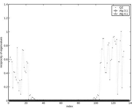
in both Algorithm 3.1 and Algorithm 4.1. However, when the standard QZ algorithm is applied to this problem, the special structure is ignored, and the reciprocity property is lost. Figure 5.2 shows the reciprocities of computed eigenvalues by three algorithms. Here the reciprocities of eigenvalues are defined by
|λiλ2n+1−i− 1|, i = 1, . . . , n, (5.2)
where λi (i = 1, . . . , 2n) are the computed eigenvalues sorted in the ascending order by
modulus.
Note that in Figure 5.2, the x-axis represents eigenvalues sorted in the ascending order by modulus. Obviously, Algorithm 3.1 and 4.1 preserve the reciprocity property, while QZ algorithm does lose the property of (5.2). It is observed that the reciprocity property by QZ algorithm is better preserved for eigenvalues near the unit circle. The behavior of three algorithms for other randomly generated examples are quite similar.
Example 2 We now consider the palindromic QEP for high-speed trains and rails. A
3D finite element model for the coefficient matrices A0 and A1 is derived by [2]. The size of
the matrices after deflation is n = 303, and the excitation frequency ω of the external force
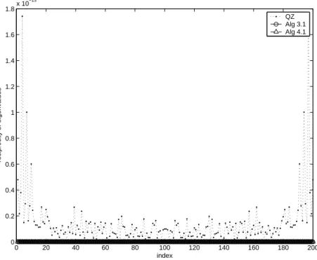
0 20 40 60 80 100 120 140 160 180 200 0 0.2 0.4 0.6 0.8 1 1.2 1.4 1.6 1.8x 10 −13 index reciprocity of eigenvalues QZ Alg 3.1 Alg 4.1
Figure 5.2: Reciprocities of computed eigenvalues of Example 1
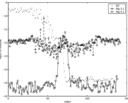
measure accuracy of an approximate eigenpair (λ, x) for (1.1), we use the residual residual =
½
kλ2A>1x + λA0x + A1xk2, if |λ| < 1,
kA>
1x + λ−1A0x + λ−2A1xk2, if |λ| ≥ 1. (5.3)
The residuals of computed eigenpairs by three algorithms for the eigenvalues with absolute
values in [10−14, 1014] are shown in Figure 5.3, where the x-axis represents eigenvalues sorted
in the ascending order by modulus.
For eigenvalues with small modulus, Algorithm 3.1 performs much better than Algorithm 4.1 and QZ algorithm. For eigenvalues with large modulus, Algorithm 3.1 performs slightly better than QZ algorithm, and both of these two perform better than Algorithm 4.1. For eigenvalues near the unit circle, all three algorithm have similar accuracy.
Algorithm 3.1 and Algorithm 4.1 have quite similar performance in Example 1, but in this example, Algorithm 3.1 performs much better than Algorithm 4.1 except for the eigenvalues near the unit circle. This is due to the Cayley transformation used in Algorithm 4.1, which
may be illustrated by the following simple example. Let a = 1014, the Cayley transformation
b = a+1a−1 gives b = 1.00000000000002 by Matlab, and the inverse Cayley transformation
˜a = b+1b−1 gives ˜a = 1.000799917193454e + 014 by Matlab with 12 digits lost. This may help
us explain why Algorithm 4.1 performs worse than Algorithm 3.1 for eigenvalues away from the unit circle, while performs similar to Algorithm 3.1 for eigenvalue near the unit circle.
0 50 100 150 −16 −15 −14 −13 −12 −11 −10 −9 index log10 of residual QZ Alg 3.1 Alg 4.1
Figure 5.3: Log10of residual of Example 2 (ω = 5)
The important reciprocity property of eigenvalues are shown in Figure 5.4. For a com-puted eigenvalue λ, the reciprocity is defined by the minimum of |µλ − 1| over all comcom-puted eigenvalues µ(6= λ).
Clearly, our algorithms preserve the essential reciprocity property as expected, while QZ algorithm has only less than 40 pairs of computed eigenvalues near the unit circle with reciprocity near zero. More precisely, even for the eigenvalues near the unit circle, the smallest
reciprocity is 4.451 × 10⁻¹⁴. And the average and maximal value of all reciprocities are 0.220
and 1.006, respectively.
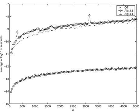
Example 3 In this example, we apply three algorithms to the palindromic QEP for high-speed trains and rails with various excitation frequency ω. Figure 5.5 shows the average of residuals of three algorithms for 100 different ω-s uniformly chosen from 50 to 5000, where
for a fixed ω, the average of residuals is defined by the mean value of the log10of the residuals
of all computed eigenpairs with eigenvalues in [10−14, 1014].
We see from Figure 5.5 that the average of residuals of Algorithm 3.1 is better than those of QZ algorithm and Algorithm 4.1 up to three to four digits for almost all ω-s.
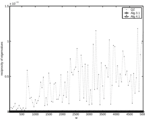
Figure 5.6 and 5.7 report the reciprocities of computed eigenvalues for ω = 50 : 50 : 5000. More precisely, Figure 5.6 reports the minimal reciprocities of eigenvalues by QZ algorithm and the average reciprocities of eigenvalues by Algorithm 3.1 and Algorithm 4.1, where for a certain ω, the average reciprocity of computed eigenvalues is the mean value of
0 20 40 60 80 100 120 140 0 0.2 0.4 0.6 0.8 1 1.2 1.4 index reciprocity of eigenvalues QZ Alg 3.1 Alg 4.1
Figure 5.4: Reciprocities of computed eigenvalues of Example 2 (ω = 5)
the reciprocities defined in (5.2). Figure 5.7 reports the average and maximal reciprocities of eigenvalues by QZ algorithm.
Figure 5.6 and 5.7 clearly show that our algorithms preserve the reciprocity property, while QZ algorithm lose this property in some sense.
6
Conclusions
In this paper, we extend the numerical approaches by the (S + S−1)-transformation and H2
-transformation for solving the real symplectic pencil and real Hamiltonian pencil to solving the >-symplectic pencil and >-Hamiltonian pencil, respectively. The extension does not hold if we extend the real case to the conjugate and complex transpose case. On the contrary, it holds if the real case is extended to the complex transpose case. The new approaches can be applied to solving the palindromic QEP with complex coefficient matrices arising from the finite element model of the high-speed trains and rails. Numerical results show that the
approach by (S + S−1)-transformation outperforms the approach by H2-transformation and
QZ algorithm.
In the future, we are also motivated to develop a structured Arnoldi-type algorithm on the
0 500 1000 1500 2000 2500 3000 3500 4000 4500 5000 −15 −14 −13 −12 −11 −10 −9 −8 −7 w
average of log10 of residuals
QZ Alg 3.1 Alg 4.1
Figure 5.5: Average of log10of residuals of Example 3 (ω = 50 : 50 : 5000)
A
Appendix
In this section we list pseudocodes of Step 2 in Algorithm 3.1 and Step 2 in Algorithm 4.1.
In the following houser(x) returns a Householder reflector H such that xH = αe>1 with α ∈
C; givensl(α,β,i) returns a Givens rotation G such that G h
α β
i
= γei with γ ∈ C; givensr(α,β,i)
returns a Givens rotation G such that [α β]G = γe>i with γ ∈ C. The functions qr(A) and
ql(A) perform the standard QR and QL factorizations.
A.1 Step 2 in Algorithm 3.1
function [ ˆK, ˆN , Q, Z] = rbutf(K, N )
Input: matrices K, N in the form (3.4)
Output: unitary Q, Z such that ˆK = QKZ, ˆN = QN Z are of the form (3.8). K, N are
overwritten by ˆK, ˆN 01: [Q1, R] ← qr(N (1 : n, 1 : n)) 02: Q ← diag(QH 1, In) 03: Z ← diag(In, ¯Q1) 04: K ← QKZ 05: N ← QN Z
500 1000 1500 2000 2500 3000 3500 4000 4500 5000 0 0.5 1 1.5x 10 −11 w reciprocity of eigenvalues QZ Alg 3.1 Alg 4.1
Figure 5.6: Reciprocities of computed
eigenval-ues of Example 3 (ω = 50 : 50 : 5000) 0 500 1000 1500 2000 2500 3000 3500 4000 4500 5000 0.2 0.4 0.6 0.8 1 1.2 1.4 1.6 w reciprocity of eigenvalues Average Maximum
Figure 5.7: Reciprocities of computed
eigenval-ues of Example 3 by QZ algorithm
06: for j = 1 : n − 2
07: for k = j + 1 : n − 1
08: % annihilate K(n + k, j) by Givens rotation in (n + k, n + k + 1) plane
09: G ←givensl(K(n + k, j), K(n + k + 1, j), 2) 10: Q(n + k : n + k + 1, :) ← GQ(n + k : n + k + 1, :) 11: K(n + k : n + k + 1, :) ← GK(n + k : n + k + 1, :) 12: N (n + k : n + k + 1, :) ← GN (n + k : n + k + 1, :) 13: Z(:, k : k + 1) ← Z(:, k : k + 1)G> 14: K(:, k : k + 1) ← K(:, k : k + 1)G> 15: N (:, k : k + 1) ← N (:, k : k + 1)G>
16: % annihilate N (k + 1, k) by Givens rotation in (k, k + 1) plane
17: G ←givensl(N (k, k), N (k + 1, k), 1) 18: Q(k : k + 1, :) ← GQ(k : k + 1, :) 19: K(k : k + 1, :) ← GK(k : k + 1, :) 20: N (k : k + 1, :) ← GN (k : k + 1, :) 21: Z(:, n + k : n + k + 1) ← Z(:, n + k : n + k + 1)G> 22: K(:, n + k : n + k + 1) ← K(:, n + k : n + k + 1)G> 23: N (:, n + k : n + k + 1) ← N (:, n + k : n + k + 1)G> 24: end
25: % annihilate M (2n, j) by Givens rotation in (n, 2n) plane
26: G ←givensl(M (n, j), N (2n, j), 1)
27: Q([n 2n], :) ← GQ([n 2n], :)
28: K([n 2n], :) ← GK([n 2n], :)
29: N ([n 2n], :) ← GN ([n 2n], :)
31: K(:, [n 2n]) ← K(:, [n 2n])GH
32: N (:, [n 2n]) ← N (:, [n 2n])GH
33: for k = n : −1 : j + 2
34: % annihilate K(k, j) by Givens rotation in (k − 1, k) plane
35: G ←givensl(K(k − 1, j), K(k, j), 1) 36: Q(k − 1 : k, :) ← GQ(k − 1 : k, :) 37: K(k − 1 : k, :) ← GK(k − 1 : k, :) 38: N (k − 1 : k, :) ← GN (k − 1 : k, :) 39: Z(:, n + k − 1 : n + k) ← Z(:, n + k − 1 : n + k)G> 40: K(:, n + k − 1 : n + k) ← K(:, n + k − 1 : n + k)G> 41: N (:, n + k − 1 : n + k) ← N (:, n + k − 1 : n + k)G>
42: % annihilate N (k, k − 1) by Givens rotation in (k − 1, k) plane
43: G ←givensr(N (k, k − 1), N (k, k), 2) 44: Q(n + k − 1 : n + k, :) ← G>Q(n + k − 1 : n + k, :) 45: K(n + k − 1 : n + k, :) ← G>K(n + k − 1 : n + k, :) 46: N (n + k − 1 : n + k, :) ← G>N (n + k − 1 : n + k, :) 47: Z(:, k − 1 : k) ← Z(:, k − 1 : k)G 48: K(:, k − 1 : k) ← K(:, k − 1 : k)G 49: N (:, k − 1 : k) ← N (:, k − 1 : k)G 50: end 51: end
A.2 Step 2 in Algorithm 4.1
function [ ˆK, ˆN , Q, U, V ] = rcf(K, N )
Input: matrices K, N from Step 1 of Algorithm 4.1
Output: unitary Q and unitary >-symplectic U, V such that ˆK = QKU, ˆN = QN V are
of the form (4.3). K, N are overwritten by ˆK, ˆN
01: [Q1, R] ← qr(K(:, 1 : n)) 02: Q ← QH 1 04: K ← QK 05: N ← QN 06: [Q2, L] ← ql(K(n + 1 : 2n, n + 1 : 2n)) 07: Q ← diag(In, QH2 )Q 08: K ← diag(In, QH2 )K 09: N ← diag(In, QH2 )N 10: U ← I2n 11: V ← I2n 06: for j = 1 : n − 1 07: for k = j : n − 1
08: % annihilate N (n + k, j) by Givens rotation from the left
10: Q(n + k : n + k + 1, :) ← GQ(n + k : n + k + 1, :)
11: K(n + k : n + k + 1, :) ← GK(n + k : n + k + 1, :)
12: N (n + k : n + k + 1, :) ← GN (n + k : n + k + 1, :)
13: % annihilate K(n + k, n + k + 1) by Givens rotation from the right
14: G ←givensr(K(n + k, n + k), K(n + k, n + k + 1), 1)
15: U (:, k : k + 1) ← U (:, k : k + 1) ¯G
16: U (:, n + k : n + k + 1) ← U (:, n + k : n + k + 1)G
17: K(:, k : k + 1) ← K(:, k : k + 1) ¯G
18: K(:, n + k : n + k + 1) ← K(:, n + k : n + k + 1)G
19: % annihilate K(k + 1, k) by Givens rotation from the left
20: G ←givensl(K(k, k), K(k + 1, k), 1)
21: Q(k : k + 1, :) ← GQ(k : k + 1, :)
22: K(k : k + 1, :) ← GK(k : k + 1, :)
23: N (k : k + 1, :) ← GN (k : k + 1, :)
24: end
25: % annihilate N (2n, j) by Givens rotation from the left
26: G ←givensl(N (n, j), N (2n, j), 1)
27: Q([n 2n], :) ← GQ([n 2n], :)
28: K([n 2n], :) ← GK([n 2n], :)
29: N ([n 2n], :) ← GN ([n 2n], :)
30: % annihilate K(2n, n) by Givens rotation from the right
31: G ←givensr(K(2n, n), K(2n, 2n), 2)
32: U (:, [n 2n]) ← U (:, [n 2n])G
33: K(:, [n 2n]) ← K(:, [n 2n])G
34: for k = n : −1 : j + 1
35: % annihilate N (k, j) by Givens rotation from the left
36: G ←givensl(N (k − 1, j), N (k, j), 1)
37: Q(k − 1 : k, :) ← GQ(k − 1 : k, :)
38: K(k − 1 : k, :) ← GK(k − 1 : k, :)
39: N (k − 1 : k, :) ← GN (k − 1 : k, :)
40: % annihilate K(k, k − 1) by Givens rotation from the right
41: G ←givensr(K(k, k − 1), K(k, k), 2)
42: U (:, k − 1 : k) ← U (:, k − 1 : k)G
43: U (:, n + k − 1 : n + k) ← U (:, n + k − 1 : n + k) ¯G
44: K(:, k − 1 : k) ← K(:, k − 1 : k)G
45: K(:, n + k − 1 : n + k) ← K(:, n + k − 1 : n + k) ¯G
46: % annihilate K(n + k − 1, n + k) by Givens rotation from the left
47: G ←givensl(K(n + k − 1, n + k), K(n + k, n + k), 2)
48: Q(n + k − 1 : n + k, :) ← GQ(n + k − 1 : n + k, :)
49: K(n + k − 1 : n + k, :) ← GK(n + k − 1 : n + k, :)
50: N (n + k − 1 : n + k, :) ← GN (n + k − 1 : n + k, :)
52: % annihilate N (n + j, j + 2 : n) by Householder reflector from the right 53: H ←houser(N (n + j, j + 1 : n)) 54: V (:, j + 1 : n) ← V (:, j + 1 : n)H 55: V (:, n + j + 1 : 2n) ← V (:, n + j + 1 : 2n) ¯H 56: N (:, j + 1 : n) ← N (:, j + 1 : n)H 57: N (:, n + j + 1 : 2n) ← N (:, n + j + 1 : 2n) ¯H
58: % annihilate N (n + j, j + 1) by Givens rotation from the right
59: G ←givensr(N (n + j, j + 1), N (n + j, n + j + 1), 2)
60: V (:, [j + 1 n + j + 1]) ← V (:, [j + 1 n + j + 1])G
61: N (:, [j + 1 n + j + 1]) ← N (:, [j + 1 n + j + 1])G
62: % annihilate N (n + j, n + j + 2 : 2n) by Householder reflector from the right
63: H ←houser(N (n + j, n + j + 1 : 2n)) 64: V (:, j + 1 : n) ← V (:, j + 1 : n) ¯H 65: V (:, n + j + 1 : 2n) ← V (:, n + j + 1 : 2n)H 66: N (:, j + 1 : n) ← N (:, j + 1 : n) ¯H 67: N (:, n + j + 1 : 2n) ← N (:, n + j + 1 : 2n)H 68: end
69: % annihilate N (2n, n) by Givens rotation from the left 70: G ←givensl(N (n, n), N (2n, n), 1)
71: Q(:, [n 2n]) ← GQ(:, [n 2n]) 72: K(:, [n 2n]) ← GK(:, [n 2n]) 73: N (:, [n 2n]) ← GN (:, [n 2n])
74: % annihilate K(2n, n) by Givens rotation from the right 75: G ←givensr(K(n, n), K(2n, n), 1)
76: U (:, [n 2n]) ← U (:, [n 2n])G 77: K(:, [n 2n]) ← K(:, [n 2n])G
References
[1] P. Benner, V. Mehrmann, H. Xu, A numerically stable, structure preserving method
for computing the eigenvalues of real Hamiltonian or symplectic pencils, Numerische
Mathematik, 78, 329-358, 1998.
[2] E.K. Chu, T.M. Hwang, W.W. Lin and C.T. Wu, Vibration of fast trains,
palindromic eigenvalue problems and structure-preserving doubling algorithms,
NCTS Tech-Report 2007-1-005, National Tsing-Hua University, Taiwan.
http://math.cts.nthu.edu.tw/Mathematics/preprints/prep2007-1-005.pdf.
[3] D. Chu, X. Liu, V. Mehrmann, A numerically backward stable method for computing the
Hamiltonian Schur form, SIAM J. Matrix Anal. Appl., to appear.
[4] G.H. Golub and C. Van Loan, Matrix Computations, Johns Hopkins University Press, Baltimore, third edition, 1996.
[5] J.J. Hench and A.J. Laub, Numerical solution of the discrete-time periodic Riccati
equa-tion, IEEE Trans. Automat. Control, 39, 1197-1210, 1994.
[6] A. Hilliges, C. Mehl and V. Mehrmann, On the solution of palindromic eigenvalue
prob-lems, In Proceedings 4th European Congress on Computational Methods in Applied
Sciences and Engineering (ECCOMAS), Jyv¨askyl¨a, Finland, 2004.
[7] T.M. Hwang, W.W. Lin and V. Mehrmann, Numerical solution of quadratic eigenvalue
problems with structure-preserving methods, SIAM J. Sci. Comput., 24(4), 1283-1302,
2003.
[8] C.F. Ipsen, Accurate eigenvalues for fast trains, SIAM News, 37, 2004.
[9] A.J. Laub, A Schur method for solving algebraic Riccati equations, IEEE Trans. Au-tomat. Control, 24, 913-921, 1979.
[10] W.W. Lin, A new method for computing the closed loop eigenvalues of a discrete-time
algebraic Riccati equation, Linear Algebra Appl., 6, 157-180, 1987.
[11] D.S. Mackey, N. Mackey, C. Mehl and V. Mehrmann, Vector spaces of linearizations for
matrix polynomials, SIAM J. Matrix Anal. Appl., 28, 971-1004, 2006.
[12] D.S. Mackey, N. Mackey, C. Mehl and V. Mehrmann, Structured polynomial eigenvalue
problems: good vibrations from good linearizations, SIAM J. Matrix Anal. Appl., 28,
1029-1051, 2006.
[13] V. Mehrmann, D. Watkins, Structure-preserving methods for computing eigenpairs of
large sparse skew-Hamiltonian/Hamiltonian pencils, SIAM J. Sci. Comput., 22,
1905-1925, 2001.
[14] C.C. Paige and C. Van Loan, A Schur decomposition for Hamiltonian matrices, Linear Algebra Appl., 14, 11-32, 1981.
[15] T. Pappas, A.J. Laub and N.R. Sandell, On the numerical solution of the discrete-time
algebraic Riccati equation, IEEE Trans. Auto. Control, 25, 631-641, 1980.
[16] R.V. Patel, On computing the eigenvalues of a symplectic pencil, Linear Algebra Appl., 188-189, 591-611, 1993.
[17] F. Tisseur and K. Meerbergen, The quadratic eigenvalue problem, SIAM Review, 43, 235-286, 2001.
[18] C. Van Loan, A symplectic method for approximating all the eigenvalues of a Hamiltonian