Adaptive piecewise linear bits estimation model for MPEG based video coding

ARTICLE NO. VC970329

Adaptive Piecewise Linear Bits Estimation Model for MPEG

Based Video Coding

Jia-Bao Cheng and Hsueh-Ming Hang

Department of Electronics Engineering, National Chiao Tung University, Hsinchu, Taiwan 300, Republic of China

Received November 6, 1995; revised July 9, 1996

flow and underflow. There are two popular types of rate In many video compression applications, it is essential to control algorithms. In the first approach, the proper quanti-control precisely the bit rate produced by the encoder. One zation stepsizes is selected based on the buffer status. That critical element in a bits/buffer control algorithm is the bits _{is, the quantization stepsize is set small when the buffer is} model that predicts the number of compressed bits when a _{nearly empty and the stepsize is set large when the buffer} certain quantization stepsize is used. In this paper, we propose

is nearly full. However, this type of control schemes such as an adaptive piecewise linear bits estimation model with a tree

RM8 and SM3 often result in non-uniform picture quality structure. Each node in the tree is associated with a linear

because (1) it does not have a bit budget plan that distrib-relationship between the compressed bits and the activity

mea-utes bits appropriately for every image block and (2) it does sure divided by stepsize. The parameters in this relationship

not take image contents into consideration in adjusting are adjusted by the least mean squares algorithm. The

effective-ness of this algorithm is demonstrated by an example of digital stepsize. Without a bit budget plan we may produce too VCR application. Simulation results indicate that this bits many bits at times; then, we have to increase stepsizes model has a fast adaptation speed even during scene changes. _{abruptly to reduce output bits. In the second case, smaller} Compared to the bits model derived from training data based _{stepsizes should be used in the smooth image region and} on cluster analysis, the adaptive piecewise linear bits model

larger stepsizes in the texture region to match the sensitiv-achieves about the same high performance with a much lower

ity thresholding characteristics of human perception. complexity and high self-adaptativity. A particular advantage

A modified version of the above scheme is to precom-of a rate control scheme employing a bits model over the

buffer-pute a budget plan for each picture frame and/or every feedback rate control such as MPEG2 Test Model 5 is that it

image block. Then, quantization stepsizes are ‘‘guessed’’ can control the bits of every microblock very precisely. 1997

based on the buffer status to produce the desired bits. One Academic Press

example of this kind of schemes is Test Model 5 (TM5) in the development of MPEG2 standards [3]. However, the 1. INTRODUCTION _{lack of an explicit bits model leads to a number of bit-rate} dependent parameters inside this scheme. Its bit control, In many video compression applications, it is essential _{bits produced for each block, is quite imprecise.}

to control precisely the bit rate produced by the encoder, _{The second type of rate control approach employs an} for example, in the cases of constant rate video

transmis-explicit bits model that describes the relationship between sion and storage. An application described at the end of

bits and quantization stepsize. This bits model is able to this paper is digital video cassette recording (DVCR). To

predict the compressed bits when a certain quantization meet the variable speed playback requirement and the

stepsize is in use before the real quantization and variable VCR mechanical restrictions, the compressed data of

spe-word-length coding (VLC) operations are actually applied cific frames have to be placed inside predefined areas.

to. In order achieve a uniform perceptual picture quality, Therefore, the coded bits generated by the encoder for

we preanalyze the entire image content and allocate bits each picture frame have to match the pre-assigned bit

accordingly. A bit budget plan is thus obtained. If the number.

predicted bit number using a selected stepsize does not In a typical motion-compensated transform coding

match the planned bit budget, the selected stepsize has to scheme such as Reference Model 8 (RM8) used by CCITT

be altered until it matches. When the bits model is accurate, expert group and Simulation Model 3 (SM3) used by ISO

the actual coded bits number is close to the predicted one motion picture expert group (MPEG) in defining video

and the bit control can thus be quite precise. Consequently, compression standards [1, 2], their output bit rate is

con-trolled by adjusting quantizer stepsize to avoid buffer over- we can encode the pictures according to the planned bit 51

1047-3203/97 $25.00 Copyright1997 by Academic Press All rights of reproduction in any form reserved

52 CHENG AND HANG

budget to produce nearly uniform image quality and, at which demonstrate the advantages of the proposed bits estimation model. A cluster analysis based approach is the same time, buffer overflow and underflow would be

eliminated. implemented for comparison. Also included is a simulation

using TM5 (of MPEG2), which produces less desirable What we have just described is a one-pass coding

struc-ture. That is, the bit budget or stepsize plan is precomputed results. At the end, a brief summary in Section 6 concludes this paper.

and then the actual quantization and VLC operations are executed once only. In contrast, we may start with a rough

guess of the stepsize and run quantization and VLC to _{2. ACTIVITY MEASURE AND CONSTANT} check the output bits. If the result is not satisfactory, we _{LINEAR MODEL}

modify the stepsize and rerun quantization and VLC again

The image activity function is a measurement of the [4]. This multiple-pass structure may be used for off-line

image content complexity; a high activity value indicates simulations; however, it is too expensive to be used in

real-a hreal-ard-to-compress imreal-age (block). Severreal-al types of real-activity time machines.

functions have been proposed. Although the block vari-There are two methods to construct a bits model. The

ance seems to be a popular activity measure ([6]), it was first method is to derive a mathematical model analytically

reported that among the following four activity measures, based on the information theory; one example of using

the one using the AC coefficient absolute values is most this method is the model proposed by Chen and Hang [5].

accurate [7]. These four tested activity measures are: The other method is to derive an experimental expression

based on test data. Because the quantizer and VLC opera- _{1. the variance of all the DCT coefficients (same as the} tions are nonlinear and the picture content is time-varying, _{block variance),}

it is rather difficult to come up with an accurate and

self-2. the sum of all the DCT coefficient absolute values, adaptive bits estimation model relying only on theoretical

3. the variance of DCT coefficients without DC term, analysis. We take the experimental approach in this paper.

and A few one-pass experimental models have been reported.

4. the sum of DCT coefficient absolute values without Puri and Aravind [6] suggested a look-up table that records

DC term. the average coded bits of the training pictures. A simple

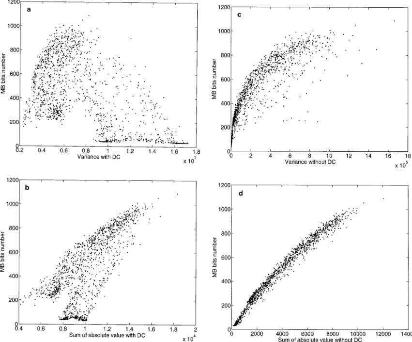
Figure 1 is the experimental results of each measurement first-order polynomial model was proposed by Sun et al.

at a fixed quantization stepsize on a picture frame of [7]. Though both schemes perform reasonably well on

con-Flowergarden sequence (CCIR601 4 : 2 : 2 format, 480 lines trolling the output buffer level, their performance degrades

by 720 pels). Each point in these figures represents the on the test pictures with characteristics different from that

coded bits and the activity value associated with a certain of the training pictures.

macroblock (MB, a 16316 image block defined in MPEG). Here, we propose an adaptive piecewise linear bits

esti-Note that the relationship between the coded bits and the mation model, whose structure is borrowed from the

tree-activity value for the fourth measure is well approximated structured piecewise linear filter in [8, 9]. Each node in

by a straight line. Hence, the fourth measure is adopted the tree is associated with a linear relationship between

as the activity measure in the rest of the paper. Mathemati-the coded bits and Mathemati-the image activity measure divided by

cally, it is defined stepsize. The parameters in this relationship can be

ad-justed by the least mean squares (LMS) algorithm.

Simula-ACT5

O

adaptation speed even during scene changes. In addition,

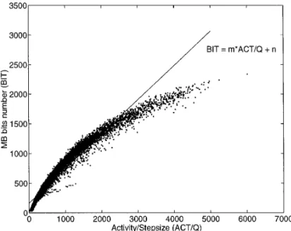
compared to the nonadaptive bits model derived from data On the other hand, given a fixed picture block, the coded using cluster analysis (in Section 5, an improved version bits for different quantization stepsizes are plotted in Fig. of [6]), the adaptive piecewise linear bits model has a much 2. The curve shows that the bit number is inversely propor-lower complexity but achieves about the same high perfor- tional to the stepsize. Combining the above experimental mance. Also, the model derived using clustering analysis results, we conclude that the number of coded bits per has difficulties in catching up the variation of data (macro)block is approximately proportional to the activity

promptly. measure and is inversely proportional to the quantization

This paper is organized as follows. The activity function stepsize. An empirical first-order bits model is thus de-used to measure the image complexity is developed in rived [7]:

Section 2. Also included is the construction of the constant coefficient linear bits model. Section 3 describes the

pro-BIT

p 5 m ACT_Q 1 n, posed adaptive piecewise linear bits model. Then, a simple

bits allocation scheme is designed in Section 4 to test the

effectiveness of the proposed model in a complete coding where BITpis the estimated coded bits, ACT is the activity measure, Q is the quantization stepsize, and m, n are two system. Section 5 presents computer simulation results

FIG. 1. (a) Coded bits versus variance with DC. (b) Coded bits versus absolute value with DC. (c) Coded bits versus variance without DC. (d) Coded bits versus absolute value without DC.

constants derived from training data to minimize a selected where i is the index of legal quantization stepsizes and j is the index of macroblocks in one picture frame. Ac-error criterion.

Typically, we choose m and n in (0) to minimize the cording to the calculus of variation, (2) is equivalent to solving both

mean square error, E[(BIT2 BITp)2_{], based on the data} triplets, (BIT, ACT, Q)’s. Each data triplet, (BIT, ACT,

Q), represents the number of coded bits, the activity value, _­

o

o

o

o

and the quantization stepsize of an image macroblock pro- _{­m ­n}

duced by the MPEG compression algorithm. For a test

picture, the above minimization process has the under rather general conditions. Thus, m and n in (2) can be calculated by solving min m,n

O

O

O

S

D

O

O

O

O

F

S

DG

54 CHENG AND HANG

FIG. 4. Variation of the linear relationship for four

neigh-FIG. 2. Coded bits versus quantization stepsize.

boring macroblocks.

and _{Fig. 3. These two drawbacks are often associated with a}

fixed empirical model derived from a set of training data.

O

O

O

Either the model is tuned to a specific set of data so that it cannot be used for the other sets of data or the model Figure 3 shows the fitness of the first-order bits estimation is loosely fit into a large set of data so that it is inaccurate model for quantization stepsizes 2 to 10. _{for a selected picture. Therefore, a more appropriate bits} There are two drawbacks of this simple first-order _{estimation model should be able to track the content} varia-model. One, the parameters, m and n, are picture-depen- _{tion of image sequence in a more precise manner. To} dent and, two, the linear expression becomes less accurate _{improve the performance of the fixed first-order model,} when ACT/Q goes beyond a certain range. The first point _{we need to develop an adaptive scheme that adjusts its} can be observed from Fig. 4, where MBiindicates the ith parameters from time to time. In addition, instead of a

macroblock in an image frame. This problem becomes _{single model that covers the entire range of data space,} more serious for blocks belonging to pictures with different _{we partition the data space (ACT, Q) into segments and} contents. The second point can be clearly observed from _{design appropriate parameter set for each segment}

sepa-rately.

3. ADAPTIVE BITS ESTIMATION MODEL

In the previous section, we have discussed a linear bits estimation model and its weak points. In this section, an adaptive bits model is proposed based on the tree-struc-tured piecewise linear filter structure. We first review the tree-structured filter which was designed for adaptive equalization in digital communication by Gelfand et al. [8, 9]. Our scheme for bits estimation application is then de-scribed.

3.1 Tree-Structured Piecewise Linear Filter

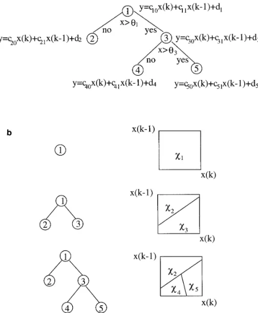
A nonlinear filter may be approximated by a piecewise linear filter in which the filter input domain is partitioned into disjoint regions and each linear filter operates only in its designated region. Figure 5 shows the structure of a piecewise linear filter [8, 9]. The input domain of this

dt, whereas the domainxt is determined by the weights

cs, offsets ds, and thresholdsusat all the ancestor nodes s

of node t.

The above point can be made more clear by examining the example shown in Fig. 6b [8, 9]. Note that there are three piecewise linear filters corresponding to the three possible pruned subtrees, namely T15 h1j, T25 h1, 2, 3j, and T35 h1, 2, 3, 4, 5j. The root node pruned subtree T1 FIG. 5. Structure of a piecewise linear filter.

corresponds to a linear filter y˜T15 y˜1. xi, i5 1, 2, . . . , N. For each arriving input x(k), the filter

output y˜ (k) is the convolution of x(k) and the impulse

The pruned subtree T2 with terminal nodes h2, 3j corre-response hi(k), where the index i is the input region that _{sponds to a piecewise linear filter comprised of two linear}

x(k) belongs to. If the input domain is partitioned using

filters restricted to two separate polygonal domains: a sequential binary split, the entire piecewise linear filter

can be organized as a tree. Each nonterminal tree node is

associated with a linear filter and a threshold value; they _y˜

T₂5

5

y˜2 if x[x2

y˜3 if x[x3. are used to split the input domain. The filter coefficients

and the threshold at each node are updated by the LMS

algorithm. One advantage of this structure is that the stan- _{The pruned subtree T}

3with terminal nodesh2, 4, 5j corre-dard linear filtering techniques can be employed at each _{sponds to a piecewise linear filter comprised of three filters} node, for example, in finding the filter coefficients. Also, _{restricted to three separate polygonal domains:}

owing to its sequential and hierarchical partitioning struc-ture, this approach is computationally efficient. It is re-ported that this filter structure has a good convergence

speed compared to many other nonlinear adaptive filters. _y˜T

35

5

y˜2 if x[x2

y˜4 if x[x4

y˜5 if x[x5. A typical example of the tree-structured piecewise linear

filter is illustrated in Fig. 6a and explained below [8, 9]. To construct a tree-structured piecewise linear filter, we

The above piecewise linear filter can be made adaptive specify three elements for each node t in the tree T: a tap

by updating the filter input domain and the filter coeffi-weight vector ct, an offset dt, and a thresholdut.

cients when new samples arrive. That is, the values of ct,

Let x be an input data vector. Then node t is associated

dt, andutare adjusted by applying the least mean squares

with a linear filter

(LMS) algorithm to the input data sequentially. A thor-ough discussion of the tree-structured piecewise linear fil-y˜t5 ct9x 1 dt,

ter can be found in [8, 9]. The version designed particularly for bits estimation is described below.

where y˜tis the filter output at node t. The final output of

this piecewise linear filter is defined by

3.2. Adaptive Piecewise Linear Bits Estimation Model In the proposed adaptive piecewise linear bits estimation y˜T5 y˜t*,

model, each node in the tree is associated with a first-order linear bits model restricted to a certain range of ACT/Q where t*_{is the terminal node in the tree T obtained through}

values. In other words, in our bits estimation model the the following process. We start from the root node and

filter output y˜ represents the estimated bits BITp. The input use the rule

vector x becomes ACT/Q (a scalar) and the coefficient vector c and the offset d are now model parameters m and y˜t.ut, go to r(t)

(5) n, respectively. Threshold u is used to restrict the active y˜t#ut, go to l(t) range of the corresponding linear bits model. Our adaptive

bits estimation algorithm is similar to the original adaptive filter algorithm in [8, 9] except for the initialization. To where r(t) is the right child stemming from node t and,

similarly, l(t), the left child. Therefore, each node in a tree ensure a reasonable initial performance, each node in the tree begins with the same parameters that are derived off-corresponds to a filter with inputs restricted to a polygonal

domain denoted by xt. In general, the filter output y˜t at line using the constant coefficient first-order bits

estima-tion model. node t is determined by the filter weight ctand the offset

56 CHENG AND HANG

FIG. 6. (a) A tree-structured piecewise linear filter. (b) Pruned subtrees and their associated input domain partition.

The adaptive algorithm for piecewise linear bits estima- Propagate the data sample from the root node to a terminal node of T according to the rule:

tion model is as follows.

BIT p

t.ut, go to r(t)

kInitializationl

Let m0 be the slope term and n0 be the bias term of the BITpt#ut, go to l(t).

initial linear bits model.

If the data sample passes through node t, then its associated We initialize each node t in the tree T by

parameters are updated:

p p pt(k1 1) 5 pt(k)1 e(1 2 pt(k)) pt(0)5 1 2depth(t), mt(k1 1) 5 mt(k)1 e pt(k1 1) (BIT(k) mt(0)5 m0, nt(0)5 n0, ut(0)5 0,

where ptis the probability of the input domain associated 2 BIT

t(k)) ACT Q (k) with node t. nt(k1 1) 5 nt(k)1 e pt(k1 1) (BIT(k)2 BITt(k)) kUpdatingl

Let (BIT(k), ACT/Q(k)) be the (k1 1)th arriving coded

data pair. Assume BITpt(k) 5 mt(k) (ACT/Q)(k) 1 u

t(k1 1) 5ut(k)1 e

pt(k1 1)

(BIT(k)2ut(k)),

where the parametere controls the convergence speed. If Therefore, this predictive type frame budget planning scheme seems to work well in our simulations.

the data sample does not pass through node t, then the

above parameters remain the same except that Once the frame bit budget is decided, we next decide the bit budget for every image macroblock inside a picture frame. In principle, we assign more bits to a macroblock pt(k1 1) 5 pt(k)2 ept(k).

of higher activity. The exact bits allocation strategy is de-scribed by

4. ADAPTIVE BITS ALLOCATION

We now describe how the adaptive bits estimation model BIT(MB0)1 BIT(MB1)1 ? ? ? 5 BITframe (7) works together with bits allocation strategy. The task of

bits allocation is to distribute bits to each macroblock prop- and erly so that the following two goals can be achieved: (1)

the total coded bits should meet the bit budget; (2) the BIT(MB0): BIT(MB1):? ? ? ₍₈₎ perceptual quality of every coded image block should be _{5 log(ACT(MB0})): log(ACT(MB1)):? ? ? , approximately equal. The above two requirements lead to

the following two additional problems: (1) how to come where MBiis the ith macroblock of a frame. Our

experi-up with an adequate bit budget for each picture frame; (2) ments indicate that the log operation in (8) would lead how to decide the proper coded image perceptual quality to a more uniform perceptual image quality. Intuitively, for every block. We do not attempt to solve these two log(ACT(MBi)) can be viewed as an information measure

additional problems thoroughly here. But rather, for dem- (in bits) of image content based on our activity function. onstration purposes, a simple yet quite effective bit budget Since the rate distortion function of a Gaussian source planning scheme is devised. Our focus is that for a given under mean square criterion has a similar log form [10], bit budget and a given picture quality measure, we want the choice of log operation seems to be reasonable. There to allocate bits to each block so that the total coded bits are several studies on how to relate the human subjective would match the preassigned bit budget. criterion to the quantization stepsizes in DCT coding (see In a MPEG coding scheme, there are three types of [11] and its references). However, since the focus of this coded frames: I-frame (intra-coded frame), P-frame (pre- paper is primarily on the bits estimation model, we adopt dictive frame), and B-frame (bidirectional frame). The I- the simple bits assignment rule defined by (8).

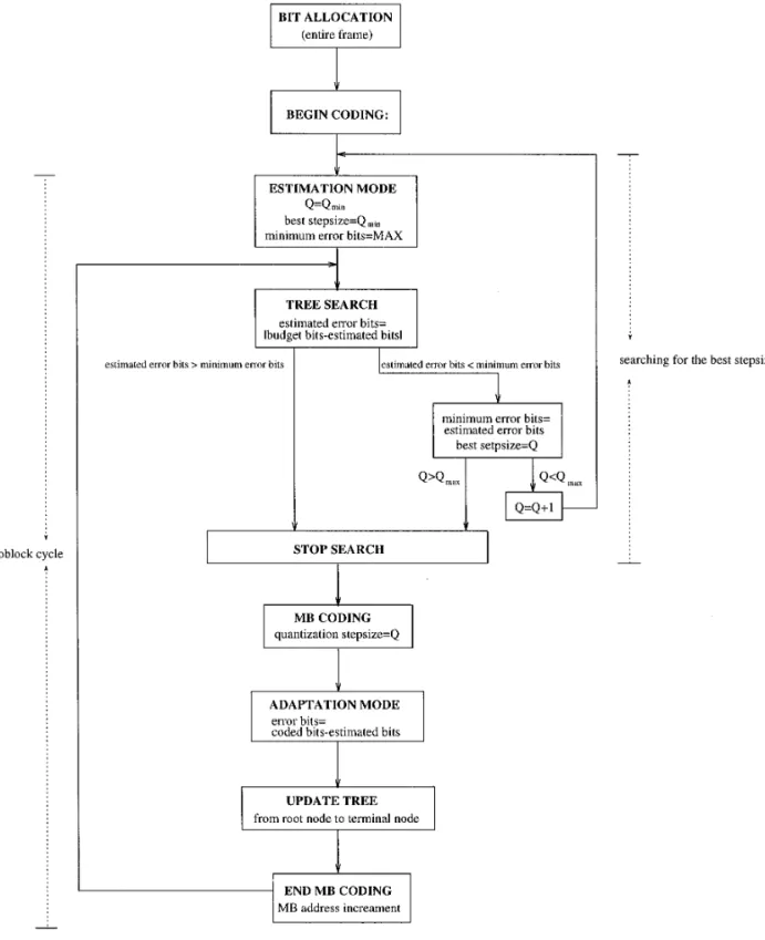
frames are independently coded and generally require the Our bits (or quantizer) control algorithm consists of two largest number of bits. The temporal redundancy in B- steps: a bits estimation step and a model updating step. In frames are estimated and removed using the already coded the bits estimation step, we look for the most appropriate P-frame(s) and/or I-frame. Therefore, the B-frames gener- stepsize that generates coded bits closest to the given bit ally require the fewest bits. An MPEG-coded sequence is budget. For a given macroblock, we first calculate its activ-partitioned into segments of pictures, called a group of ity measure (ACT). Then, we guess an initial stepsize value pictures (GOP). Typically, a GOP contains an I-frame and (Q). The ratio ACT/Q is the input to the piecewise linear

several P- and B-frames. bits model. This input, ACT/Q, propagates from the root

Our bit budget planning strategy is as follows. Assume node to a particular terminal node according to (5) and our GOP structure is fixed; that is, the numbers and posi- the estimated bit number is the output of the terminal tions of the P- and B-frames in one GOP are known and node. If the estimated bit number does not match the pre-unchanged. For a given average bit rate per second, we selected bit budget, the stepsize is increased or decreased thus know the bit budget of a GOP, which is called BITGOP. (according to the bit difference) and the previous process Then, the distribution of bits among the I-, P-, and B- is repeated. A flowchart describing this procedure is shown

frames are in Fig. 7. The best stepsize is the one that produces the

estimated bits closest to the bit budget. Then we use the BITI: BITP: BITB5 ACTI: ACTP: ACTB, (6) estimated stepsize to quantize the current macroblock. In the model updating step, the bit estimation error, which is the difference between the coded bits and the estimated where ACTIis the total activity measure of the I-frame,

and ACTP and ACTB are the frame activity measures of bits, is used to update the piecewise linear bits estimation model. The model parameters are modified by the LMS the P- and B-frames averaged over all the P- and B-frames

in one GOP. In theory, we could precompute the activity algorithm described in the previous section. This completes the encoding of one macroblock as shown in the flowchart measures of the entire GOP and then perform coding

oper-ations. However, to reduce implementation complexity, of Fig. 7. In the meantime, the activity measure of every block is collected and at the end of this GOP the frame we simply use the previous GOP activity attributes for

planning the bit budget of the next GOP. Even at scene total activity will be used to update the bit budget distribu-tion for the next GOP.

58 CHENG AND HANG

FIG. 7. Flowchart of bit estimation and model updating.

There are three main advantages of using the tree-struc- provides ‘‘piecewise’’ adaptation. It means that when each training sample arrives, we update the parameters of the tured filter structure. First, the piecewise linear filter is

clearly superior to the single linear filter in solving nonlin- nodes that are located on a data-dependent path from the root node to a terminal node. As a result, only a small ear problems. Second, since the tree structure employs

standard linear adaptive filtering techniques at each node, portion of nodes in the tree should be modified and the other nodes remain unchanged. Meanwhile, the updating it is simpler than many other nonlinear adaptive filters,

such as polynomial filters. Third, the most important fea- process modifies slightly the domain of the corresponding filter and those of its neighbors. Hence, the whole process ture of the tree-structured adaptive algorithm is that it

is simple yet effective. Since the bits model is gradually

BIT

p 5 0.58 ACT_Q 1 164 for I-macroblock dominated by the newly arrived coding macroblocks, the

influence of the far-away blocks becomes less important.

This also matches the locality characteristics of images. _BITp 5 1.00 ACT

Q 2 38 for P-macroblock 5. SIMULATIONS

BIT

p 5 1.13 ACT_Q 2 92 for B-macroblock The target application of our computer simulations is

digital video cassette recording (DVCR) [12, 13]. Because

of the mechanical limitations (magnetic heads and tape _{(A scaling factor may have to be inserted in applying the} movement) there are special requirements posed by _{above formulas to different pictures.) In the adaptive} DVCR system [12]. In order to implement variable speed _{model, the tree depth is three so that the corresponding} playback and in the meanwhile retain a high compression _{piecewise linear bits estimation models have adequate} efficiency, we have proposed a modified MPEG compres- _{complexity. Larger tree depths have been test without} sig-sion algorithm dedicated to DVCR application [13]. To _{nificant improvement. Before an image sequence is coded,} enable fast playback, a short GOP containing only one _{the tree-structured bits estimation models are initialized} I-, one B-, and one P-frames is chosen. According to the _{using the constant linear bits models, which are obtained} ‘‘Consumer-use DVCR Specifications’’ [14], the bite rate _{off-line from encoding the first three image frames.} How-for the standard TV (CCIR601) DVCR is 25 Mbps. Assum- _{ever, because of the adaptivity of the tree-structured bits} ing that the audio and the other digital data would need _{model, any reasonable constant model can be used as the} 2 Mbps, the video data bit rate is thus around 23 Mbps or _{initial values. They all shortly converge to the model of} 2.3 Mbits for each GOP. In this particular application, the _{the processed data.}

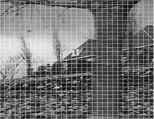
coded bits have to be carefully controlled to match the _{In the following discussions, the error bits are defined} exact bits assignment because data have to be placed at _{as the difference between the coded bits and the estimated} the exact location to facilitate the variable playback re- _{bits for each macroblock. Because P-frames are typically} quirement (scanning heads read in data only on the regu- _{dominated by P-macroblocks and B-frames are dominated} larly spaced specific locations). This application is an exam- _{by B-macroblocks, for convenience, our statistics are} per-ple used to demonstrate a potential use of our bits model _{formed on the entire picture rather than on different types} and rate control algorithm. It can certainly be used for the _{of blocks. In Fig. 9, we first show the absolute error bits} other applications that require accurate bit rate control. _{with and without adaptation for the I-frames in encoding} The bit budget of each macroblock is determined at the _{the video sequence Flowergarden. The horizontal axis is} beginning of encoding a picture frame. Figure 8 shows a _{the accumulated macroblock (MB) number. Since one} pic-typical example of bit budget distribution. For the conve- _{ture contains 1350 MBs, the portion in Fig. 9 is the end of} nience of comparison, the original picture is split into mac- _{the second I-frame and the beginning of the third I-frame.} roblocks in accordance with the bit budget distribution. _{They are the fourth and the seventh pictures in the original} One may notice that the more complicated (high activity) _{sequence. In the cases of ‘‘without adaptation’’ we simply} macroblock is assigned more bits. However, since the log _{use the constant estimation models described previously.} operation is used in (8), the bit budget increases slowly in _{It is clear from this figure that the adaptive piecewise linear} the high activity regions. This may be justified from a _{bits estimation model decreases the error bits significantly.} perceptual viewpoint that coding errors are often less visi- _{Similar performance improvement is obtained also for} P-ble in high variance regions. From our experiments, the _{frames and B-frames (Figs. 10 and 11). The stepsize} adjust-picture quality using log scale is better than that without it. _{ment parametere for I-macroblocks, P-macroblocks, and} B-macroblocks is 0.01, 0.001, and 0.001, respectively. These 5.1. Constant versus Adaptive Models

values are decided empirically to maintain a reasonable speed of convergence, typically around a few hundred mac-Because the coding behavior is rather different for

intra-coded macroblocks (I-macroblocks), P-frame predictive- roblocks.

In Fig. 12, we demonstrate the adaptation ability of the coded macroblocks (P-macroblocks), and B-frame

pre-dictive-coded macroblocks (B-macroblocks) in MPEG proposed piecewise linear bits estimators when scene change occurs. In the middle of the test sequence (the coding, three tree-structured bits estimation models are

separately constructed. For comparison and initialization 150th frame), the scene changes from Flowergarden to Football. The adaptive bits model is able to adjust its pa-purposes, the constant coefficient first-order linear model

is also derived from the data. A typical example of the rameters rapidly to cope with picture variation, whereas the constant model has a significant higher average error constant coefficient model for the Flowergarden

param-60 CHENG AND HANG

FIG. 8. An example of bit budget distribution.

eters can be used as the initial values of this piecewise 5.2. Adaptive versus Table-Lookup Models linear model without degrading its long-term performance.

Table 1 is the average absolute error bits per macroblock Although the previous simulation results demonstrate the advantages of the adaptive bits estimation model over with and without adaptation. For example, in encoding

the third image sequence composed of Flowergarden and the constant coefficient model, we like to make one more comparison against a complicated yet potentially better Football, the error bits are reduced by 60% for I-frame,

same TABLE1 entry are further divided into M subcells based on their Q values. Thus we obtain a new table with entry (Tbl2BIT, Tbl2ACT, Tbl2Q), where Tbl2BIT and

Tbl2ACTare the average bits and activity values of all the

coding data triplets classified to the same TABLE1 entry (Tbl1BIT, Tbl1ACT/Q) but with different quantization

step-size Q. This new table is called TABLE2.

Using clustering analysis, we divide the coding data space into many small regions (cells) in hoping that with appropriate choice of features (ACT and Q) the bits num-ber in each small region (cell) is close to each other. Conse-quently, we could estimate the bit number based on the feature space partition specified by TABLE2. In other words, given an input MB, we first compute its activity

FIG. 9. The prediction error bits (absolute values) per mac-roblock of I-frame (a) using a constant-coefficient linear model and (b) using an adaptive piecewise linear model.

on clustering analysis. First, we collect the data pairs in the form of (BIT, ACT/Q) and generate a table that con-tains the representatives of these data pairs using the K-means cluster algorithm [15, 16]. In other words, we chose a cluster number, say K; then, the iterative K-means proce-dure partitions the data samples into K cells, each centers around a representative. We continue modifying the cell representatives until the total square distance between the cell members and their representatives reaches a (local) minimum point. In our case, the representatives are de-noted by (Tbl1BIT, Tbl1ACT/Q). They are entries in

TABLE1. Then, we expand the dimension of each entry _{FIG. 10. The prediction error bits (absolute values) per} mac-in the TABLE1 mac-into the form of (Tbl2BIT, Tbl2ACT, Tbl2Q). roblock of P-frame (a) using a constant-coefficient linear model, and

(b) using an adaptive piecewise linear model.

62 CHENG AND HANG

value, act, and then for each possible quantization stepsize, q, we search this table to find the entry (Tbl2BIT, Tbl2ACT,

Tbl2Q) in which the Tbl2Q value matches q exactly and

the Tbl2ACTvalue is closest to act; then, the Tbl2BITvalue

in that entry represents the estimated bits. Other than the fact that BIT, ACT, and Q are strongly related, this bits model does not assume a particular underlying relationship among BIT, ACT, and Q. In encoding an image sequence, (ACT, Q) acts as an index in searching the bits table. These features make this table lookup approach rather different from the previous adaptive bits estimation model. In the proposed adaptive piecewise linear bits model, we assume that the relationship between BIT and ACT/Q is nearly linear, and in the process of searching for the target linear

FIG. 12. The prediction error bits (absolute values) per mac-roblock at scene change (a) using a constant-coefficient linear model and (b) using an adaptive piecewise linear model.

bits estimation model we use ACT/Q not (ACT, Q). Other arrangements in table construction have been tested, but they produce less favorable results, such as constructing TABLE2 without constructing TABLE1 first. This may be due to the uneven distribution of data samples and, thus, performing the clustering operation directly on (BIT, ACT, Q) space leads to biased partitions.

Table 2 shows the average absolute error bits produced by the table lookup approach with different table sizes. The first two columns are the numbers of entries of TABLE1 and TABLE2. Because in our coding system the

FIG. 11. The prediction error bits (absolute values) per

mac-reasonable choice of Q could be any integer value from 1

roblock of B-frame (a) using a constant-coefficient linear model and

TABLE 1

The Average Absolute Error Bits per Macroblock of Flowergarden, Football, and

Flowergarden1 Football with/without Adaptation Using (piecewise) Linear Model

I-frame P-frame B-frame

Image sequence Without With Without With Without With

Flowergarden 149 60 83 39 54 43

Football 80 53 123 78 109 63

Flower1 Football 146 57 107 58 74 52

of TABLE1. In the cases of which TABLE2 sizes are garden and Football, respectively. Also shown in Figs. 13 greater than 480, their average absolute error bits are com- and 14 are the TM5 simulation results which will be ex-parable with those of the adaptive bits estimation model plained in the next subsection. The fixed model designed in Table 1. However, there are no benefits to increase the for Q between 2 and 10 predicts fewer bits than the coder lookup table size beyond 960. The limitation comes from actually produces in the range of stepsizes used in simula-the uncertainty between simula-the activity measure and simula-the cod- tion. Hence, the coded bits are constantly higher than ing bits for a macroblock. That is, two macroblocks of the the budget.

same activity value may produce different bit numbers. The motion compensation technique is quite effective Unless we use a better activity measure (with less uncer- _{in compressing the Flowergarden sequence because it is a} tainty), we could not further reduce the bit errors. _{panning image sequence. Since the image content is not} When Table 1 is compared to Table 2, the adaptive bits _{changing very much between nearby frames, the fixed bits} estimation model not only approaches the same perfor- _{model is off the target, but it is still quite stable. In contrast,} mance limit, but it also uses a much smaller size memory _{the Football sequence has fast, multiple object movement.} than the table-lookup method. For example, the number _{Because its content changes rapidly, the motion estimation} of nodes in adaptive modeling is 15 for a tree of depth _{is not as effective. The fixed model fails in catching up} three, whereas the table size is 960 in the lookup-table _{with the changes. On the other hand, the adaptive bit} approach. Also, the calculation required to produce a bit _{estimation scheme controls the output bits rather precisely} estimate is less for the adaptive bits estimation scheme. It _{to match the design target. For reference, we also include} takes three comparisons and three first-order linear equa- _{the coded bits distribution of each frame of our proposed} tions in the adaptive bits model, but it takes 32 comparisons _{scheme (Figs. 15 and 16) and the average PSNR (Table} in the 960-entry lookup-table scheme. Most importantly,

3). The effectiveness of motion compensation can also be it is not easy to make the lookup table approach adaptive.

observed from Figs. 15 and 16. To keep an equal PSNR for I-, P-, and B-frames, the bit rates of all these three

5.3. Complete Coding Systems _{types of frames in the Football sequence are almost equal,}

while the bit rates of the P- and B-frames are much smaller Finally we show the results of our complete MPEG

cod-than that of the I-frame in the Flowergarden sequence. ing system using the proposed bits estimation model for

Because the coded pictures have rather high PSNR (35 to rate/buffer control. Figures 13 and 14 show the bits

distri-butions per GOP, with and without adaptation for Flower- 40 dB), as one may expect, their subjective quality is very

TABLE 2

The Average Absolute Error Bits per Macroblock of Flowergarden, and Football Using Clustering/Table Method

Flowergarden Football

TABLE1 TABLE2

size size I-frame P-frame B-frame I-frame P-frame B-frame

16 480 83 65 50 72 78 73

32 960 68 43 35 57 63 58

64 1920 63 41 40 61 70 66

64 CHENG AND HANG

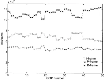
FIG. 15. Bits distribution of I-frames, P-frames, and B-frames for Flowergarden using an adaptive bit model.

FIG. 13. Bits distribution of GOP for Flowergarden.

good. Therefore, the reconstructed pictures are not

in-cluded in the paper. tion of the quantization stepsize. TM5 decides the stepsize

based on the buffer feedback information and the block

5.4. MPEG2 Test Model 5 _{activity measurement. It does not employ a bits model,}

whereas our scheme decides the stepsize based on the bits At the end, we simulate the MPEG test model 5 (TM5,

model (and the block activity measurement that deter-Rev. 2 in [3]) for comparison purposes. A typical rate/

mines the allocated bits of a block). There is no explicit buffer control procedure can be split into two stages: bit

use of buffer feedback information in our scheme, although allocation and quantization stepsize selection. Although

it may also be included to further increase the preciseness the activity (image complexity) measures are different in

of rate control and to prevent the buffer from overflow TM5 and our scheme, the basic concepts behind their bit

and underflow in the case of model breakdown in practi-allocation algorithms are similar. The major difference

be-tween the TM5 and our rate control schemes is the selec- cal systems.

FIG. 16. Bits distributions of I-frames, P-frames, and B-frames for Football using an adaptive bit model.

TABLE 3

The Average PSNR of Flowergarden and Football (150 Frames/Sequence)

I-frame P-frame B-frame

Image

sequence Y Cr Cb Y Cr Cb Y Cr Cb

Flowergarden 34.8 32.2 29.6 34.7 31.9 29.5 35.6 32.2 29.6

Football 40.4 37.5 32.7 40.5 37.4 32.7 40.7 37.4 32.8

We review very briefly here the basic elements in the bit budget. In our scheme, the stepsize is chosen solely based on our bits model to meet the bit budget. Therefore, TM5 rate control scheme. Its complete description is

te-dious and is referred to [3]. The TM5 encoder also adheres it becomes very critical in our scheme to have an accurate bits model.

to the single-pass coding philosophy. In other words, the

current frame and GOP bit allocation is predicted by using Another interesting point is that the complication in the TM5 rate control algorithm is due to the sophisti-the previously coded frame(s) and GOP information. The

image complexity (or activity) measure (X) at the frame cated formulas in calculating various parameters such as d and Nact. The complication in our rate control is level is estimated based on the product of the average

macroblock quantization stepsize (Q) and the number of due to bits model updating. Because Nact calculation in TM5 requires computing eight block variances, the coded bits (S) of the previous picture (of the same picture

type); that is, X5 Q 3 S. Three image complexity measures TM5 rate control seems to be more demanding in computing power.

are computed for the I-, P-, and B-frames separately.

Al-though the exact formula in TM5 is more complicated in Because the purpose of this simulation is to compare the rate control algorithms, we did not activate the more allocating the bits for each picture frame, its basic principle

is similar to that of our frame bit allocation scheme (Eq. advanced features in MPEG2 coding such as field estima-tion and field DCT. The TM5 simulaestima-tion results using the (6)).

The MB quantization stepsize in TM5 are decided by same coding parameters as before (bit rate, IPB structure, etc.) are shown in Figs. 13 and 14. Figures 13 and 14 indicate two factors: (1) the deviation from the planned buffer

full-ness, d; (2) the normalized MB activity, Nact. After the that when the picture content is rather nonuniform such as in the case of Flowergarden sequence, the bit rate of total bits of a frame are decided, TM5 further assumes the

bits are evenly distributed for the entire picture. The virtual individual GOP varies quite significantly. This is due to the fact that the even distribution of MB bits over the buffer fullness predicted by the preceding assumption is

the planned buffer fullness. Again, three virtual buffers, entire image is not valid in this case. The upper half of Flowergarden is the smooth sky and the lower half is the one for each picture type, are used. The second factor, MB

activity, is calculated based on the minimum variance of deep texture flower bed. The control parameter adjustment based on buffer fullness does not respond quick enough the four luminance 83 8 frame blocks and the

correspond-ing four luminance 83 8 field blocks of the original picture. to match the image content changes. This phenomenon can be clearly observed from Fig. 17, which shows the The variance measure is then normalized against the

aver-age variance of the most recently coded picture to produce (virtual I-frame) buffer fullness after every MB is coded. The goal of TM5 control is try to keep the buffer fullness Nact. Several constants are involved in the above

calcula-tions. Eventually, the MB quantization stepsize is a product curve nearly constant. In the case of Flowergarden, it gener-ates too few bits in the upper half of the picture and it of a scaled buffer fullness deviation d and the normalized

MB activity Nact. generates too many bits in the lower half. It turns out,

in this particular frame, that the total bits is higher than Comparing our quantization scheme with the one in

TM5, we observe two major differences. The first one is expected at the end of the picture. In contrast, the moving objects and the background in the Football image are pretty the MB bits are assumed to be evenly distributed in TM5,

but the MB bits in our scheme are decided by the MB much evenly distributed. Thus the buffer-fullness based TM5 rate control works quite well. Its buffer status is activity (Eq. (8)). However, the MB activity still enters

into the TM5 stepsize selection through a multiplicative nearly flat in Fig. 17. The weakness of a buffer-feedback rate control scheme is that, although it may keep a long-factor (Nact). The second and more significant difference

is that the TM5 stepsize is mainly decided by the buffer term average rate close to the desired (one GOP, say), it usually cannot control bits precisely for every MB to meet fullness deviation (the normalized MB activity does not

66 CHENG AND HANG

increase the stability and preciseness of our rate control scheme with a simple feedback mechanism.

REFERENCES

1. CCITT, Working Party XV/4, Description of Ref. Model 8 (RM8), June 1989.

2. ISO/IEC JTCI/SC2/WG11, Doc. MPEG 90/41, MPEG video

simula-tion model three (SM3), April 1991.

3. ISO/IEC JTCI/SC29/WG11, Doc. NO400 Test Model 5, April 1993. 4. L. Wang, Bit rate control for hybrid DPCM/DCT video codec, IEEE

Trans. Circuits Systems Video Technol. 4, No. 5, 1994, 509–517.

5. J.-J. Chen and H.-M. Hang, A transform video coder source model and its applications, IEEE Int. Conf. Image Processing ’94, Austin,

Texas, Nov. 1994, pp. 967–971.

6. A. Puri and R. Aravind, Motion-compensated video coding with adaptive perceptual quantization, IEEE Trans. Circuits System Video

Technol., 1, No. 4, 1991, 351–361.

7. W.-Y. Sun, H.-M. Hang, and C.-B. Fong, Scene adaptive parameters selection for MPEG syntax based HDTV coding, in Int’l Workshop

FIG. 17. Buffer status under TM5 rate control: 36th picture

(I-on HDTV ’93, Ottawa, Canada, Oct. 1993.

frame) of Flowergarden and 12th picture (I-frame) of Football.

8. S. B. Gelfand, C. S. Ravishankar, and E. J. Delp, Tree-structured piecewise linear adaptive equalization, IEEE Trans. Commun. 41,

6. CONCLUSIONS

1993, 70–82.

9. S. B. Gelfand and C. S. Ravishankar, Tree-structured piecewise linear In this paper, we propose a bits estimation model with

adaptive filter, IEEE Trans. Inform. Theory 39, 1993, 1907–1922. self-adaptation ability for real-time video coding. The tree

10. T. Berger, Rate Distortion Theory, Prentice Hall, Englewood Cliffs, structure of the adaptive bits estimation model provides

NJ, 1971. a fast search for the best quantization stepsize and easy

11. H.-Y. Gong and H.-M. Hang, Scene analysis for DCT image coding, updating of the bits model. Experiments show that the

in Int’l Workshop on HDTV ’93, Ottawa, Canada, Oct. 1993. number of error bits of the adaptive bits model decreases

12. S.-W. Wu and A. Gersho, Rate-constrained optimal block-adaptive significantly as compared to the simple nonadaptive linear _{coding for digital tape recording of HDTV, IEEE Trans. Circuits} bits model. It is observed that this adaptation model is _{Systems Video Technol. 1, No. 1, 1991, 100–112.}

able to adjust itself quickly even at scene changes. _{13. J.-B. Cheng, H.-M. Hang, and D. W. Lin, An image compression} We also compare the adaptive bits estimation scheme scheme for digital video cassette recording, in IEEE International

Conference on Consumer Electronics, Chicago, June 1994, 26–27. with the bits model obtained using a clustering/table

14. F. Azadegan et al., ‘‘Data-placement procedure for multi-speed digital method. The latter bits model is a lookup table with entries

VCR, IEEE Trans. Consumer Electron. 40, No. 3, 1994, 250-256. storing the precomputed bits, activity, and quantization

15. J. A. Hartigan, Clustering Algorithms, Wiley, New York, 1975. stepsize values. Simulation results indicate that the error

16. W. R. Dillon and M. Goldstein, Multivariate Analysis: Methods and bits of the adaptive bits model is comparable with that of

Applications, Wiley, New York, 1984. the clustering/table model designed for a selected

se-quence. However, the adaptive bits model has a much lower complexity and is able to update its parameters to match the time-varying data.

At the end of the Simulation section, the experimental results using TM5 (of MPEG2) are included as a reference. The rate control scheme in TM5 is designed based on the buffer feedback concept. This type of schemes may work reasonably well, when properly designed, on maintaining long-term average bit rate and preventing the buffer from underflow or overflow. However, if we wish to have a

JIA-BAO CHENG received her B.S. and M.S. degrees in Electrical precise control on the bits for every microblock, either a

Engineering from National Chiao Tung University, Hsinchu, Taiwan in trial-and-error approach or a precise bits model has to be

1992 and 1994, respectively. From 1994 to 1995, she was with CCL/ employed. Because the focus of our paper is on the bits

ITRI, Hsinchu, Taiwan, where she was a multimedium system engineer. model, the simple rate control scheme we propose does _{Currently, she is an IC design engineer in SD Micro Co., Hsinchu, Taiwan.} not include a buffer feedback mechanism. Its success relies _{Her research interests include image/signal processing algorithms and}

ar-chitecture. solely on the accuracy of the bits model. We could further

in digital image compression algorithm and architecture research. He joined the Electronics Engineering Department of National Chiao Tung University, Hsinchu, Taiwan in December 1991. His current research interests include digital video compression, image/signal pro-cessing algorithms and architecture, and digital communication theory. Dr. Hang was a conference co-chair of the Symposium on Visual

Communications and Image Processing (VCIP), 1993, and the Program

Chair of the same conference in 1995. He guest coedited two Optical

Engineering special issues on Visual Communications and Image Pro-cessing in July 1991 and July 1993. He was an associate editor of IEEE Transactions on Image Processing from 1992 to 1994 and a

co-HSUEH-MING HANG received his B.S. degree and M.S. degree from

National Chiao Tung University, Hsinchu, Taiwan in 1978 and 1980, editor of the Handbook of Visual Communications (Academic Press, 1995). He is currently an editor of Journal of Visual Communication respectively, and his Ph.D. in Electrical Engineering from Rensselaer

Polytechnic Institute, Troy, NY in 1984. From 1984 to 1991, he was and Image Representation, Academic Press. He is a senior member

of IEEE and a member of Sigma Xi. with AT&T Bell Laboratories, Holmdel, NJ, where he was engaged