Pulsatile flow in a rotating straight pipe: I. Analysis of the fluid motion
inside a nutation fluid damper
U. Leia) and C F Ho . .
Institute of Applied Mechanics, National Taiwan University, Taipei 106, Taiwan, Republic of China (Received 13 January 1992; accepted 22 June 1993)
Rigorous analysis shows that the spin synchronous mode fluid motion inside a nutation fluid damper on board of a spinning satellite can be modeled as an incompressible, laminar pulsatile flow in a circular straight pipe. The pipe rotates with constant angular velocity w about an axis perpendicular to its own axis. The distance between the rotation axis and the pipe axis is much greater than a, the pipe’s radius. The flow is driven by a three-dimensional harmonic oscillation of the pipe wall with frequency a and amplitude wh, and is governed by three-dimensionless parameters: R, ( =&/Y) , A ( =o/s2), and A ( = w@a ) , where Y is the kinematic viscosity of the fluid. Both the asymptotic analysis and the numerical calculation have been carried out for Ro==O.l-1000 and A=O-2 under A< 1. It is found that the rotating effect increases the energy dissipation significantly in comparison with the result of the pulsatile straight pipe flow in an inertia frame (the previous theory for the nutation damper). For A = 1.5, the energy dissipation in a rotating pipe flow is 5.43 times that in a “stationary” pipe flow for large Rn, which agrees with the previous experiment. A steady stream is induced by the convective effect for finite values of A. Such steady motion is consisted of axial counter flows together with pairs of counter-rotating vortices in the cross-sectional plane.
1. INTRODUCTION
Study of this problem is motivated by the analysis of the fluid motion inside a nutation fluid damper on a freely precessing satellite, as shown in Fig. 1. Let (X,, Yb ,Z,) be the Cartesian coordinate system fixed to the satellite with the origin 0 at its mass center. Assume that the satellite is axisymmetric about the Z, axis, with the axial moment of inertia J greater than the transverse moment of inertia I. Here the transverse direction is perpendicular to the Z, axis. The system spins about the symmetric axis for system stabilization and attitude control, and possesses minimum total kinetic energy when the nutation angle, 8, equals zero. When 8=0, the direction of the angular velocity (0) coincides with that of the angular momentum H( = Jg) . A transverse impulse of angular momentum Hi ( 1 g1 1 4 1 @I ) may be applied to the system if one wish to change the pointing direction of the spinning axis, say, from a given direction in space to 00’ in Fig. 1. In such a case, the magnitude of the angular momentum of the spinning sys- tem remains unchanged after the impulsive angular mo- mentum has been applied, but the direction of the angular momentum does change to the 00’ direction, and does not coincide with the direction of the instantaneous angular velocity. The satellite thus undergoes a gyroscopic motion about the 00’ axis, and possesses excess energy in com- parison with the energy for the purely spinning system when 8=0. Figure 1 sketches an instantaneous picture of such gyroscopic motion with finite 0. As in Carrier and Miles,’ the precessing angular velocity pz (J/I)we^’ and the spinning angular velocity about the Z, axis
“IAuthor to whom correspondence should be addressed.
Qz ( 1 - J/I)w?’ provided that 8 is sufficiently less than unity, which occurs in many practical systems. Here, 8” and e^’ are the unit vectors along the OZh and 00’ direc- tions, respectively. Note that ~+Qse for 84 1. For the present study, J> I, Q is in the opposite direction of w and E. Referring to the (X,, Yb,Zb) coordinates in Fig. 1, the angular momentum (&?=He^‘) may be decomposed into two components, one along the spin axis (HP?‘) and one along the transverse direction (H&$), where & is the unit vector along the transverse direction. One way to remove the unwanted gyroscopic motion is to install a passive nu- tation fluid damper on the satellite to transfer energy from the transverse axis (associated with Ht) to the spin axis, and to damp out the excess energy of the gyroscopic sys- tem (see Cartwright et al. ‘) .
A nutation fluid damper is a hollow tube formed into closed shapes, usually into a torus or ring, and filled or partly filled with a fluid with certain viscosity. The fluid filled inside the damper is mercury for many practical dampers. When the damper performs properly, the system undergoes a decaying gyroscopic motion with the nutation angle decays with time. Figure 1 shows a partly filled damper mounted with its axis parallel to the spin axis of the satellite, which is the same as those studied by Alfriend and Cartwright et aL4 Here the axis of the damper is defined as the normal of the plane formed by the centerline of the closed tube which passes through the mass center of the empty damper. The mass center of the empty damper is denoted by 0” in Fig. 1 and is at a distance h from the mass center of the satellite along the axis of the system. In some systems such as that studied by Bhuta and Koval,5 the damper may be mounted with its axis perpen-
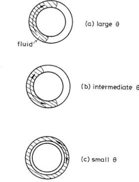
(a) large 0 flui
(b) intermediate 8
.- Yb
FIG. 1. Sketch of a nutation damper on board of a freely precessing satellite.
dicular to the spin axis of the satellite (see Fig. 2). In the present paper, we shall study the parallel installed damper formed by a circular tube with radius a which is coiled into a circle with radius R. Whenever the spin axis of the sys- tem does not coincide with the direction of angular mo- mentum, the system undergoes gyroscopic motion and thus drives the fluid inside the damper via the motion of the damper wall. The fluid motion relative to the wall of the damper dissipate the energy of the system, and hence reduces the nutation angle. Finally, the spin axis coincides with the direction of the constant angular momentum, and the fluid inside the damper undergoes rigid body rotation.
For 6J#O, there are three types of fluid motion in a partly filled mercury damper for the parallel installed case, namely, the nutation synchronous mode, the spin synchro-
=b =b
w h!
;@ Yb $& yb
(a) lb)
FIG. 2. Sketch for the installations of the dampers: (a) parallel installed case, the points A, B, C, and D are on the X,Y, plane; (b) perpendicular installed case, the points A, B, C, and D are on the YJ,, plane.
(c) small 8
FIG. 3. Three types of fluid motion in a partly Elled nutation fluid damper: (a) nutation synchronous mode, (b) spin synchronous mode,
(c) “ring” mode.
nous mode and the “ring” mode, which occur in sequences as 0 decreases (see Fig. 3). The first two modes were named after Cartright et al4 For relative large values of 8, the fluid lumps into a slug and moves unidirectionary with respect to the wall of the damper, and is called the nutation synchronous mode. For sufficiently small 19 (say, less than OS”, as suggested by Carrier and Miles’), the fluid is spread out over the outer part of the damper and formed a continuous ring pattern. Here we call it the ring mode. The fluid in the ring mode oscillates sinusoidally, with respect to the pipe wall due to the nutation effect. Both the nuta- tion mode and the ring mode were first studied by Carrier and Miles’ and Miles.6 They employed the energy-sink method to determine the decay time constant of the nuta- tion angle, and hence most of their effort is to determine the energy dissipation associated with the relative fluid mo- tion inside the damper. Later, Cartwright et al4 pointed out that in the intermediate range of 0, there exists another mode that the fluid behaves as a slug but oscillates sinuso- idally with respect to the wall, and they called it the spin synchronous mode. The fluid motion transits smoothly from the nutation synchronous mode to the spin synchro- nous mode, and then to the ring mode as the nutation angle decreases. Finally, 0 is reduced to zero and the fluid un- dergoes rigid body rotation. On some satellites (see Alfriend3), the center of the damper is offset from the spin axis so that the fluid will always behave as a slug. Alfriend investigated the dynamics of the satellite for both the nu- tation synchronous mode and the spin synchronous mode by modeling the fluid as a rigid slug of finite length. The fluid slug is assumed to experience a drag force which is related to the fluid motion inside the damper. The drag
force is assumed to be proportional to the relative velocity between the slug and the wall. The proportional constant is determined by the shear stress of the fluid motion at the wall for the nutation synchronous mode, and by the aver- age energy dissipation rate associated with the fluid motion for the spin synchronous mode. Based on the above as- sumptions, Alfriend obtained the time history for the decay of the nutation angle. For the spin synchronous mode, Alfriend compared his theoretical damping constant with Hraster’s’ experimental findings (see Alfriend*), and found that the experimental results were 1.85 to 9.97 times the theoretical values for different cases, which implies that the theory predicts a much larger time constant for the d&cay of the nutation angle. The descrepancy between Al- friend’s theory and Hraster’s experiment may be due to the following reasons: ( 1) the fluid mechanics analysis for es- timating. the rate of energy dissipation, (2) the dynamic model suggested by Alfriend, and (3) the accuracy of the experiments.
The present study try to clear up the above discrep- ancy between the experiments and the theory for the spin synchronous mode by reconsidering only the fluid mechan- ics analysis. Alfriend did not study the fluid mechanics in detail, but employed the result of Bhuta and Kova? to determine the damping constant in his dynamic model. Bhuta and Koval’ studied a fully filled damper which is installed with its axis perpendicular to the spin axis of the satellite [see Fig. 2(b)]. Based on the situation that the fluid oscillates back and forth, with respect to the wall, and the radius of the tube is much less than the radius of cur- vature of the damper, Bhuta and Koval modeled the fluid motion inside the damper as pulsatile flow inside an infinite circular straight pipe driven by a harmonic axial oscillation of the pipe wall. The flow is laminar and axisymmetric based on Bhuta and Koval’s model. The axial velocity is the only nonzero velocity component, which is simply gov- erned by the diffusion equation and solved via the Laplace transform technique. The average energy dissipation per cycle of the pipe wall oscillation was then obtained and employed to determine the decay time constant for nuta- tion via the energy-sink method. Bhuta and Koval also did some experiments and found that their theoretical predic- tions on the decay time constant of the nutation angle (which is inverse proportional to the energy dissipation) are 9% and 15% higher than the measurements when the rotation Reynolds number Rn [defined in Eq. (6)] equals to 8.3 and 7, respectively.
Alfriend3?* employed Bhuta and Koval’s’ stationary straight pipe flow model to study the dynamics of a spin- ning satellite with a partly filled damper, which is mounted with its axis parallel to the spin axis of the satellite [see Fig. 2(a)] when Ro=218-873 and A=1.5 and 2. Here A is a frequency ratio parameter and is defined in Eq. (6). The adjective “stationary” is employed in this paper to empha- size that the pipe flow in Bhuta and Koval’s model occurs in an inertial frame. The reason that Alfriend’s theoretical result does not agree with Hraster’s’ experiment can be study by considering the differences between the stationary straight pipe flow model proposed by Bhuta and Koval and
the flow situation in the damper studied by Alfriend. Ad- ditional (important) effects can then be included in Bhuta and Koval’s model to form a new fluid model. Some of the obvious effects are ( 1) rotating effect-the pulsate fluid motion inside the damper occurs actually in a noninertial frame (a frame which is mainly rotating with the vector sum of the precessing and the spinning angular velocities of the system) instead in an inertial frame studied by Bhuta and Koval; (2) curvature effect-the damper is a closed curved pipe; (3) end effects of the fluid slug for a partly filled damper; (4) unstable and turbulent effect-the flow inside the damper may be unstable or even turbulent for some of the parameter regimes of the spinning system.
We shall not consider the fourth effect here partly be- cause we do not have a comprehensive understanding on the instability and turbulence of the unsteady rotating flow, and partly because some of the parameter regimes of prac- tical interest are laminar. The analysis of the third effect is difficult because of the existence of the interface; the dy- namics of the contact angle had to be considered (see Dussang). However, the third effect is expected to be not important on the energy dissipation as soon as the length of the fluid slug is sufficiently greater than the radius (a) of the cross-sectional area of the damper, which is valid for many dampers in practical situation. Both the Coriolis force associated with the first effect and the centrifugal force associated with the second effect may generate a sec- ondary flow in the cross-sectional plane of the damper. The increase of the energy dissipation due to the secondary flow generated by the curvature effect in the pulsating curved pipe flow in an inertial frame is 0( 10%) of the stationary straight pipe result (see Berger et al. lo>. Such increase is not important in comparison with the discrepancy in the energy dissipation in Alfriend’s case mentioned above, which is 0( 100%) of the stationary straight pipe result. The increase of the energy dissipation due to the’secondary flow associated with the rotating effect is not clear since the pulsate pipe flow in a rotating frame has not been studied previously, at least up to the authors’ knowledge. However, the unidirectional flow in a circular straight pipe rotating with constant angular velocity (e) about an axis perpen- dicular to its own axis had been studied quite extensively. Both the experimental measurements by Ito and Nanbu” and the numerical calculations by Lei and Hsu” showed that the friction factor can be increased up to three times of the corresponding stationary pipe flow results due to the rotating effect for large values of oa’/y, where Y is the kinematic viscosity of the fluid. Hence, it is encouraged to include the first effect in the present study.
In case the end effects of the fluid slug can be ne- glected, the analysis of the fluid motion for the spin syn- chronous mode in a partly filled damper is essentially the same as that in a fully filled damper. Let 4 be the time rate of change of the nutation angle. When 14 I( 1 Q 1 z 1~ 1
t cdi 3 -. .- \- w - _.“_~_ ~- VI XI
FIG. 4. Configuration of the Row inside a nutation fluid damper. (X,, Y,,Z,) is an inertial Cartesian coordinates. (r’&) is a toroidal coordinates rotating with constant angular velocity OX?“, where I” is a unit vector along the 2, direction. Also, &, is the prescribed velocity of the pipe wall associated with the nutation effect, which drives the fluid motion inside the curved pipe.
fluid motion inside the damper can be approximated as quasisteady (see Carrier and Miles’). Referring to the par- allel installed case in Fig. 1, the motion of the wall of the damper for 6% 1 is mainly rotating with k cos ~+QzGx?“, with superimposed small amplitude oscillation associated with the nutation effect. The quasisteady fluid motion in- side a parallel installed, fully filled damper can be approx- imated as the curved pipe flow problem in a frame rotating with angular velocity we”” in Fig. 4. A right-handed toroi- da1 coordinates (r’,a,p) in the frame rotating with WY is employed in the present study. The nutation effect is re- 0ected by the eccentric motion of point 0” around the 00’ axis in Fig. 1, and is taken into account through a deriva- tion similar to that in Carrier and Miles’ as
z&= [WE, sin(&‘+fi)cos CZ]~?~,-- [WA sin(fit’
+/3)sin cr]&- [wh cos(Clt’+fi)]fSp, (1) which is a three-dimensional oscillation of the pipe wall. Here wh = phtl, t’ is the time, and +, ca, and Zfi are the unit vectors along the r’, CII, and /3 directions, respectively. A rigorous analysis in Sec. II will show that the flow in Fig. 4 is governed by four-dimensionless parameters: the curva- ture parameter 6( =a/R), the amplitude parameter A[= wg(&)], the frequency ratio A( =o/fL) and the ro- tation Reynolds number R, ( = aa’/v) . For practical situ- ations, S=O( 10-l) -O( lo-‘). Under the condition 641, the rotating curved pipe flow problem in Fig: 4 can be reduced to the rotating straight pipe flow problem in Fig. 5 governed only by three parameters: A, A, and Ra. Note that the rotating effect on the fluid motion is much more significant in the parallel installed damper (Alfriend’s case) than that in the perpendicular installed damper
(Bhuta and Koval’s case). This is because w is always perpendicular to the axial flow for all the positions along the centerline of the damper for the parallel installed case in Fig. 2(a), and thus the Coriolis effect is maximized. On the other hand, the Coriolis force varies along the pipe
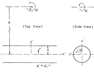
R
I (Top View) (Side View)
FIG. 5. The rotating straight pipe flow modeI. (x’,y’,z’) and (J,(T,z’) are the rotating Cartesian and cylindrical coordinates fixed, with respect to the pipe wall. The direction of 0 is parallel to the y’ direction. The distance between the rotation axis and they’ axis, R, is much greater than the radius of the pipe, a.
from zero at location A (and C) to a maximum value at location B (and D) for the perpendicular installed case shown in Fig. 2(b).
The work of the present paper is to analyze the fluid motion in Fig. 5 under the assumption for small values of A, with particular emphasis on the energy dissipation as- sociated with the relative fluid motion. The result will be compared’ with Hraster’s’ experiment to check if the rotat- ing pipe flow model works. We shall consider the “fully developed” case, which is the case that the flow field is independent of the axial coordinate (z’ in Fig. 5 or fi in Fig. 4). Beside the above application in the aerospace in- dustry, it is hoped that the nature of a pulsate pipe flow in
.
a rotating frame, m particular the nature of the secondary flow, is of interest to some of the researchers in fluid me- chanics.
This paper is the first part of the work on the pulsatile flow in a rotating straight pipe, which includes the formu- lation of the problem in Sec. II, the linear analysis based on A-g 1 in Sec. III, the asymptotic solutions in Sec. IV, the numerical solutions in Sec. V, a remark on the axial oscil- lation problem in Sec. VI, and a conclusion in Sec. VII. The cases for A = O( 1) have also been studied by solving numerically the unsteady, NavierStokes and continuity equations, and the results will be reported separately as Part II of the work on pulsatile flow in a rotating straight pipe.
II. FORMULATION
Consider the fluid motion inside a fully filled damper as shown in Fig. 4. The governing equations for the flow of a Newtonian 0uid with constant density p and kinematic viscosity Y in the rotating toroidal coordinates (r’,a$) are
3~’ u’ R+2r’cos a
i ad
v’ sin a 13W’
p+7
R+r’ cos a +r’da-R+r’cosa-‘(R+r’cosa)-co
dfi ’(24
ad
ad
dad
r2
I2
w3“’
ar’+r’aat(R+r:‘cos
a) $&-Rw~r~~o~a+2mwf
‘OS a
1 &I’” 1 d sin a 1
a2d
=--
p3Tv
- ~-.
r’ da R+r’ cos a -(R+r’ cos a)‘%a5.d
cos aad
-
&‘iJfi’(R+r’ cos a) a$’
)I
’CW
ad
VI ad
p
ad
dd
r2 .
bt)-bU’ ~+;;~+(R+~.~~~
a)
~+7-+RJ+r:c~;a-2mw’ sin a1 ap’*
=---
pr’ aa
1
a2d
1a2d
sin aad
r’ cos a)‘&?-’ r (R+r’ cos a) @G’a+(R+r’ cos a)2 d/3
g+RJ?c:s a
ad U' i ad
~“~-paa
)I
9(2b)
(2c)
ad
aw’ U’W ’ cos
ad aw’
v’w’ sin a IdW’
x+”
F+R+r’
cos a+j;;z-R+r!
cos a+ (R+r.cos a)
-@+2mu’sin a-hu' cos a1
ad
)I
1
apf*
(R+r’ cosa) 3 -p(R+r’ cosa) dfi ’
(2d)
where ( u’,v’,w’) are the velocity components in the rotat- Coriolis force oU& oR oR
ing (r’,a,/3) frame, centrifugal force -7r-y-g-,,,* w. /R
(
t2
p’*=p’+p r’R+kcos a CO’ cos a
)
is the reduced pressure which absorbs the centrifugal force due to the rotation, andp’ is the pressure. Equations (2a)-
(2d) are the continuity and Navier-Stokes equations in the rotating toroidal coordinates system. The corresponding equations in an inertial frame can be found from Berger et al. lo Note that the gravity has been neglected in the above formulation, which is valid for a satellite operating in the space environment. The boundary conditions for Eqs. (2a)-(2d) are
As w/,u= 0( 1) and R$ he for most of the systems under consideration, the Coriolis force is much greater than the centrifugal force. On balancing the Coriolis term and the unsteady term in Eqs. (2b) or (2c), one finds that v~-Uf-(w/n>w’-w’ for w/8=0( l), which is valid for most of the systems of interest. Also the boundary condi- tions shown in Eq. (1) indicate that U’ - v’ - w’
- WA. Hence, Eqs. (2a)-(2e) are normalized by introduc- ing
~‘~~~+v’t?~,-tw’i?~=g~ at r‘==a, (2e)
(u’,v’,w’) r’
(u,ww) =
4 3 r=-, a where z& is given by Eq. ( 1) . No initial condition is given
here since we shall seek only the long-time response of the flow field, i.e., the quasisteady solution.
The axial ftow (w’) and the flow in the cross-sectional plane (u’,v’) are coupled to each other through both the Coriolis force and the centrifugal force. The relative im- portance between these two forces is
P I* t=t’$-J, p*=---
paflw& ’
The resulting dimensionless equations are
(3)
1 av Sv sin a S aw
-=o
+TZ-l+Srcosa+(l+Srcosa)
afi
’
SW
au v2 Sw” cos a---_
(l+Srcosa)afi r l+Srcosa +2Aw cos a
ap* i id S sin a
= _-__
--_-
~
dr Rn raa l+Srcosa
s2
a221
Sa2w
6~0~
aw
-(l+Srcosa)‘@+ l+Srcosa &S/3+(1+Srcosa) - ap
)I
’SW
av uv
SW2 sin a(l+Srcosa)dp+r+ l+Srcosa -2Aw sin a
s2
a2v
S
d2W S’sinaaw
-(1+2Srcoscr)Zdp2-r(1+Srcosa) dflda+(l+Srcosa)2t@
)(
a0
v iau
ZG’+T7FG
)I
’aw SUWCOS~ vaw SVW sina
U3F+1+Srcosa+~ZG- l+Srcosa+(l+Srcosa:) $T +2Avsina~2Aucosa
aw
Sw cos aTG+l+Srcosa
(54
_ a+l
( I(
S au ia S av Sap*
---
dr r (l+Srcosa)@ ) r& i (l+Srcosa) Z@
)I
-(l+Srcosa) w’with boundary conditions
u=sin(t+~)cos a, v= -sin(t+/?)sin a,
w= -cos(t+fi) at >=I, where
(6)
are the four dimensionless parameters governing the fluid motion. For practical situations such as those studied by Alfriend,3*8
S=O( 10-s) -O( lo-‘), A=O( 10-I) -O( l),
A=O(lj, Rn=O(lO)-O(103).
As S is always of or less than 0( lo-‘), one may sim- plify the analysis by setting S-+0. Equations (5aj-( 5d) then reduce to au u I av -$;;+;+--z=O, (74 au ( au v
au v2
%+A u a~+;~-7 +2Aw cos a
) ap* = --_--- dr 0)
(5b)
(5c)(5d)
I 1 a av v i au = -;gfRa, s+;-;&, cl ( 1 (7c) 1 a2w 1 aw I a2w ==R n dlz+Tar+zG (7d)Equations (7aj-(7dj depict a loosely coiled pipe limit of the flow in Fig. 4. Note that Eqs. (7a)-(7d) are also the “exact” governing equations for the pulsating “fully devel- oped” flow in a straight pipe which lies on a constant rotating table (see Fig. 5), with w representing the velocity component along the z’ axis. Here the fully developed flow means that the flow is independent of the axial location of the straight pipe. The rotation axjs is parallel to they’ axis and passes through the point 0” in Fig. 5. The distance between the axis of the pipe and the rotation axis is R, which is much greater than the pipe’s radius, a. As the flow described by Eqs. (7a)-(7d) is independent of the axial coordinate z’ in Fig. 5 (or fi in Fig. 4 for S( 1 ), the bound- ary conditions for Eqs. (7a)-(7d) that are consistent with Eq. (5e) are
u=sin t cos a, v= -sin t sin a,
w=-cost at r=l. Ue) The rotating pipe flow model described by Eqs. (7a)-(7e) and Fig. 5 is a remedy for Bhuta and Koval’s5 stationary pipe flow model proposed in the present study. The gov- erning equation for the stationary (straight) pipe flow model, according to Bhuta and Koval,’ is
g=-& ($+j$), (84
subjected to
w( 1,t) =o, t-CO; w(l,t)=--cos t, t>O. (8b) The flow is axisymmetric for the stationary straight pipe flow model. On the other hand, one can find that
u(r,a,t)=u(r,2a-a,t), v(r,a,t) = -v(r,23--a,t), Pa) w(r,a,t) =w(r,27r--a,t), p*(r,a,t) ==p*(r,2n.-a?)
(9b) for the rotating straight pipe model by inspecting Eqs.
(7a)-(7e). The rest of this paper is to study the rotating pipe flow model under further assumptions.
There are two differences between the stationary pipe flow model and the rotating pipe flow model arising from the rotating effect: ( 1) The stationary pipe flow model has only the axial velocity component while the rotating pipe flow model is three dimensional even if the rotating pipe flow is driven only by an axial harmonic oscillation of the pipe wall. The axial flow is coupled with the “secondary flow” in the cross-sectional plane through the Coriolis and the convective effects. (2) The flow in the rotating pipe flow model is driven by a three-dimensional harmonic os- cillation [see Eq. (7e)] of the pipe wall, while the pipe wall of the stationary pipe flow model performs only an axial harmonic oscillation [see Eq. (8b)]. Note that the radial and the circumferential components of the pipe wall oscil- lation have no effect on the energy dissipation for the sta- tionary pipe flow model.
Equation (7a) is satisfied automatically by introducing a stream function I/ such that
1 a*
w
u=--
rda’ v=-ar’
(10)
The pressure gradient terms can also be eliminated by tak- ing cross differentiation of Eqs. (7b) and (7~). The equa- tions of motion then become
& V2$-& V2Vz~f2A $ sin a+: g cos a
(114
aw i
.~-RV’W-~A 1 a* a*
n yzcosa+ssinct
where V2 is the Laplacian operator in the (~,a) plane and 3(*,*)/3(r,a> is the Jacobian operator. The boundary conditions for Eqs. ( 1 la) and ( 1 lb) can be derived from Eqs. (7e) and (10) as
$=sin t sin a, w . . ar=sm t sm a7 w=-cos t at r=l.
According to Eqs. (lla)-( llc), we have
.$(r,a,t) = -$(r,2n--a$), w(r,a,t) =w(r,25----a&. (12) The three-dimensional oscillation problem described by Eqs. ( 1 la)-( 1 lc) can be transformed into an equiva- lent axial oscillation problem by setting
*=+h w=a-wR, (13)
where
zjR=r sin t sin a, wR= -2A cos t (14)
describes a rigid body motion. By substituting Eq. ( 13) into Eqs. (1 la)-( 1 lc), we obtain
& V2$-& V2V2$+2A 2 sin a+: g cos a
A ac&v$ +achv%
Ez-
(
30-d
1
’
r iW,a)(154
ai- i
x--~V’w”-2Aia&
-
R ;zcosa+$sinaA a&a
a(ha
=-
r ( d(r,a) + d(r,a) ’ with i&o, $=o,(15b)
W= (2A- 1)cos t at r= 1. (15c)For the equivalent axial oscillation problem described by Eqs. ( 15a)-( 15c), the axial velocity component i% will be called the primary flow while the flow in the (r,a) plane associated with $ will be called the secondary flow for the later discussion in this paper.
The dimensionless local rate of energy dissipation per unit mass associated with the relative fluid motion in the rotating straight pipe flow model in Fig. 5 is
CD’ Q>= 7 vwh-/a’ =2( ($)2+[~(~+U)]2]+(~~)2+(92
+[ig+r$ (:)I2
-21 (92+[; (~+9]2]+(;92+(P)2=A 1 a(484
r 3(r,a) ’(lib)
(16)The difference between the function Cp for the rotating straight pipe flow model in Fig. 5 and that for the rotating curved pipe flow model in Fig. 4 is of order 0(S2). Both Bhuta and Kova15 and Alfriend employed a dimensionless function g to characterize the average normalized energy dissipation per cycle of the pipe wall oscillation. For the present rotating pipe flow model under the quasisteady condition, we need only to consider the flow variation dur- ing one cycle of the pipe wall oscillation. In terms of the present notation,
g=gR E’
=A s,‘”
LY”
L1
Q(r,a,t;Rn,A,A)rdrda dt, (17) where E’ is the energy dissipated per unit axial length of the fluid during one cycle of the pipe wall oscillation, and M’ =pru2 is the mass per unit axial length of the fluid in the pipe. Here we employed the subscript “R” for g in Eq. (17) to refer that it is based on the rotating pipe flow model. Also, g is a function of Rn , A and A for the present rotating pipe flow model, but is only function of R, for the stationary pipe flow model proposed by Bhuta and Koval(which will be denoted by gs in the later discussion). The velocity components of the rigid body motion
1 atCIR
uR=--=sin t cos a,
r aa
III. LINEAR ANALYSIS
In case the wall oscillates with low amplitude but high frequency, the parameter A is small, and we may set
&(r,aJ) =%(r,a,t) +A&(r,a,t) +A’42(r,~,t) +. . . (194 and
6(r,a,t) =$r,a,t) +Afil (r,a,t) +A%&(r,a,t) +. * * . (19b) The assumption for small values of A is valid for some systems and for most of the systems at the final stage of nutation decay. By substituting Eqs. (19a) and (19b) into Eqs. (15a)-( 15c), and after certain manipulations, we ob- tain the following systems of linear equations:
; v2&-& v2v2&
GOa)
aw,
i aw,
~sina+;~cosa ,
aw, i
z3-V2i&=2A ;zcosa+!$sina
ia&
-
, (2Ob)n
with boundary conditions
&=o, $0,
i&= (2A- l)cost
at ~=l,(2Oc) and
a$R . (184
uR=-x=-sm tsin a, WR= -2h CO.3 t &V2&-&V2V2&+2A
aiz,
~sinaft~cosatogether with the pressure
&=(4A2-l)rcosacost+const (18b)
satisfy Eqs. (Ila) and (llb). If further A=O.5, they also satisfy Eq. ( 1 lc). It follows that
i&o, w=o
is a solution for Eqs. (15a)-( 15~) when A=O.5. There is no deformation and, hence, no energy dissipation when A=O.5 in the present rotating pipe flow model. For the linear case when A =O, the energy dissipation for the ro- tating pipe flow model is roughly (2A - 1) 2 times that for the stationary pipe flow model, according to Eqs. (15~) and (8b). Therefore, the energy dissipation predicted by the rotating pipe flow model may be greater or less than that predicted by the stationary pipe flow model, depend- ing on the magnitude of A. For the practical cases such as those studied by Alfriend,3’8 A= 1.5 and 2, and, hence, (2A- I)‘=4 and 9, respectively. The rotating pipe flow model predicts much more energy dissipation in compar- ing with that predicted by the stationary pipe flow model, and thus agrees better with Hraster’s’ experiments.
awl I
x-~V~i&--2A1 ai&
4,
n pzcosa+zsina ’(21a)
(2lb)
with boundary conditions:
- a&
+1=-=i&=O at r=l.
& (21c)
Recall from Eq. ( 12) that we have conditions imposed on the line a=0 (or P) for the general nonlinear flow gov- erned by Eqs. ( 1 la)-( 1 lc). For the linearized flow quan- tities &, & ,...., and z$,, Gt ,.... in Eqs. ( 19a) and ( 19b), we have
&(r,a,t) =zi&(r,2n-a,t),
Gr,a,t) = -&(r,2rr--a,t),
(224
&(r,a,t) =&(r,21~--a,t), .w
h(r,a,tj = -h(r,2a-a,t), (22bj
as well as
Gdr,W> =GAr,+a,tj, &-Jr,cr,t> =&(r,r-a,t), Wa) Zl(r,a,t>=-z&(r,n--a,t),
&;(r,a,t) = -&(r,n-a,t> (23bj
by inspecting Eqs. (20a)-(20c) and (21a)-(21c). Hence, we need to consider only the flow in the first quadrant of Fig. 5 for analyzing the linearized flow field.
Solving Eqs. (20a)-(20c) is equivalent to solving the following complex problem:
& v2*$--&
v2v2*;
a@
iawg
arsina+;xcosa ,
(244
) (24b)
with
t,h$=O, ?$=O, wz=(2A-l)e’f at r=l, (24~)
where r,$ and w$ are complex functions of r, a, and t, and
&=Re(#), &=Re(w$j, (25)
are the solutions of Rqs. (20a)-( 2Oc). Equations (24a)- (24~) suggest that the quasisteady solution takes the form
@(r,a,t) =&(r,a)e”, w$(r,a,t) =z&(r,a)eif, (26) where &, and zZe are complex functions of r and a in gen- eral. On substituting Eq. (26) into Eqs. (24a)-( 24c), we obtain
1
iV2&-- V2V2qo= -2A
azo
i aw,
&I -sin ar a+- r da - cos a
(274
1
i$,--- V2r.ij0=2A 1 ai& 46
h-l -- r aa: cos a+- dr sin a (27bj with
$c=!$=&- (2A- 1) =0 at r= 1. (27~)
On writing
-- -
+O = $or+ ilc0i 9 ii& = li& + il&i , (27dj
and using Eqs. (25) and (26), we have
?/JO = &J~ COS t- ~Oi sin t, 6s = Gcor COS t - lzioi sin t.
(28) Thus the source terms on the right-hand sides of Eqs.
(21a) and (21b) can be written as
(294
a~o,v2~oj
+wk9v2~o)
d(r,a> d(r,a> = Bo+ B1 cos 2t+ B2
sin
2t, with aciJor,v2Gorj +a(3;0i9V2$0ij a(r,a> d(w) aV2&;oi f3V2.1j;oi-7sina+---=g-rcosa
B =L
a($oOr,v2~00r)
’ 2r
a(~oj,v2~oj) I avVoisin a
%,a)
-
%,a>
da
avVooi
-arrcoSa
,
acv2~o,,,$o,ij +W2$0i,40A +avVor .
%,a>
%,a>
-z-
sm a
avVor
-drrcosa ’
1
and = Co + Cl cos 2t + C2 sin 2t, (29bj withc =A a($o,,,~o,) ~~iJooi~~oi) aEoi .
’ 2r %,a) + d(r,a) -XS’na
d&i
+drrcosa 1 ’
I
C1=z;
a(~oOr,~Orj
d(r,a) -a(i50i,coij aGoi .
a(r,a) +daSma&i$,i
-drrcosa ’
1
1
c2=zy
a(E0,,$0ija(w)
+a(~Oi,iJoTj d(r,a) +aaor da ‘lna .azor
--rcosa .
ar 1
These source terms suggest that the first-order compo- nents, $t and wl, in Eqs. (21a)-(21c), can be expressed as
$t(r,a,tj =hdr,aj +Re[~dr,ak”il
+Im[&(r,aPl,
(304
$(r,a,t) =EIS(r,a) +Re[ziJ,(r,a)e”‘]
+Im[@b(r,a)e”‘]. (3Obj
The primary interest for the first-order result is that the pulsating driving mechanism [see Eq,( 15c)] can generate a steady stream (denoted by 6,s and $ts) via the nonlinear
convection terms. By using Eqs. (30a) a@ (30b) and which implies that gR is a weak function of A for small (21a)-(21cj, the governing equations for ($rs,W,,) are values of A.
-&V2V2&s+2A %sina+i%cosa =Bo,
(314
a&, .
- cosa+ ar sina =C,, (3lb) with- a&,
1cll.F ar
-=i&=O at r=l.For small values of A, the dimensionless rate of energy dissipation per unit mass, @, can be expressed as
@=@,+A@,+O(A2), (32) where
(334
andav,
+5Y r
( )I
with-
1 &ii
q=- -,
r aaG=
[tfj$+rg (:)I],
Gi -a~; i=O,l.(33b)
Consequently,&=&+Ag,+O(A2j,
(344
according to Eq. ( 17)) where go and gl are associated with Q. and @i, respectively. With Eqs. (25)) (26), (30a), and (30b), each term on the right-hand side of Eq. (33b) can be written in the following form:
Q1= [ p(r,a)cos t+f’(r,a)sin t] [ f2(r,a> +f3(r,a)cos 2t+f4(r,a)sin 2t].
where jc,
f’, f”, f”,
and f” are related to (~o,iTo,iiYo) and (Gi ,& & j together with their spatial derivatives. It follows thata=& s,“”
6 J-i
Q>,(r,a,cR,A)r dr da dt=O. Hence,2414 Phys. Fluids A, Vol. 5, No. IO, October 1993
IV. ASYMPTOTIC SOLUTIONS
Perturbation solutions are obtained in this section for the limiting cases RQN 1 and Rn$ 1 with finite values of A and small values of A.
A. Asymptotic solution for Rn41
Consider first the zeroth-order solution. For small Rn, we may expand the solutions for Eqs. (27a)-(27c) by reg- ular perturbation series as
~&‘,a> =&&,a) +k&(r,a) +&&(r,a)
+R&&(r,a)+-*- , (354
Wr,a> =r7jodr,aj +Rn&(r,a) +&i&(r,a)
fR&i&(r,a)+~~~ . (35bj
The governing equations for qoo, qool, qo2,... and Woo, Goi, ii&,... are obtained by substituting Eqs. (35a) and (35b) into Eqs. (27aj-( 27c), and collecting the terms of equal powers of Rn. The solutions up to the third order are
$O=iJOOr+i$Oi
A(2A- 1) = Ri 4608 (6r-131$+8?--r’jsin a A(2A- 1) 192 (r-23+J)sin a (3W 1,s (-3+4$-r4) R:, f$(2-I)+- 2304 ( 19-27rZ+9r4-P) R3 A2 +& (2-6?+6r4-2r6) R; +E A2(5?-8r4+3p6)cos 2a)I
. (36bjIt follows from Eq (36aj that the maximum value of $ai equals 1.491~ lo-“A(2A- l)R& which occurs at r=0.4472, a =90”, and the maximum value of qoo, equals
3.606x 10⁻⁴(2A-l)~;, which occurs at r=0.4352,
a=90”. When Ro=O.l and A= 1, the numerical results in Sec. V for the maximum values of $ci and Goo, together with their locations are 1.5~ low5 (r=0.45, a=90“) and 3.6~ lo-’ (r=0.425, a=90”), respectively, which agree nicely with the asymptotic results.
It is interest to see the first-order steady term ($ls,GtS) associated with the effect of tinite values of A. The source terms on the right-hand sides of Eqs. (3 la) and (31b) can be evaluated by using Eqs. (36a) and (36b) as
B =b(2A-l)
0
16 Rf$ sin 2a+O(R4,),c =W--1)
0 4 Rnr cos a+O(RL).
With these source terms, a simple scaling analysis of Eqs. (31a) and (31b) shows that wls-Ri and +bls-R~. Thus the equations governing the leading-order terms, according to Eqs. (31a) and (31b), are
-’ V2V2&s+2A
aloIs
1 awls
Rn ap sin a+-- r da cos a
=R 2 n A(2f6m1) 3 sin 2a,
(2A- 1)
-& V2iZls=RQ 4 ycos a.
(37d
(37b)
Although the steady stream, z&s and $ts, are generated by the source terms associated with the nonlinear convection effect, &.s and $rs are coupled together through the Cori- olis terms in general according to Eqs. (3 la) and (31b). However, Eqs. (31a) and (31b) red_uce to Eqs. (37a) and
(37b) as Rn* 0, and thus Wts and $rs are decoupled from each other. The distribution of WIs is mainly due to the source term, according to Eq. (37b), but the distribution of $ts depends on both the source term and the Coriolis term in Eq. (37a). The solution of Eqs. (37a) and (37b) subject to Eq. (31~) are
(2A- l)A
“‘=( 3072 ( -?+2r4-r6)sin 2a
+W;),
(38a)
W,s= (2A-1)
32 (r-?>cos a Rh-tO(R$. (38b)
The associated velocity components of the steady second- ary flow are
1 wls
i&p- ~
r da (2A-1)A z 1536 (-r+2?-?)cos 2a ai& &E -- & (38~) (2A-1)A = 1536 (r-4?+3?)sin 2a(38d)
Equations (38a)-(38d) show that the steady stream is consisted of a counter flow along the axial direction and two pairs of symmetric counter-rotating vortices in the cross-sectional plane. Note that GIs is symmetric about the x’ axis in Fig. 5 but antisymmetric about they’ axis, while
$rs is antisymmetric about both the x’ and y’ axes, accord- ing to Eqs. (22b) and (23b). When 2A- 1 is positive, the axial flow is positive in the first and the fourth quadrants of Fig. 5,’ but is negative in the second and the third quad- rants. Such axial flow direction is reversed if 2A - 1 is neg- ative. The directions of the counter-rotating vorticies can be identified from the sign of ZIs along a=0 and a =r in Eq. (38~). Here, GIs is negative along a=0 but is positive along a=r/2 when 2A- 1 > 0, and vice versa when 2A
-1 <o.
The normalized energy dissipation per cycle according to Eqs. ( 17a) and (34b) for R,< 1 is
On the other hand, the result, according to the stationary pipe flow model in the limit R,+O, is
RQ 11
-g--~&+O(& ,
(39b)
which can be obtained by using Alfriend’s result, or by solving the quasisteady solution of Eqs. (8a) and (8b) using regular perturbation expansion for small value of Rn . Here the subscript “0” for both gR and gs is employed to refer that gR and gs are evaluated under the asymptotic condition R o-0. It follows from Eqs. (39a) and (39b) that
I-&A2R;+O(R4,)
(40) which equals to unity when A =0, decreases as A increases from zero, equals to zero when A=0.5, and then increases approximately with (2A - 1 )2 when A > 0.5 provided that R&A2/576 is sufficiently less than unity.
B. Asymptotic solution for R&l
As R,= O( 102) -O( 103) for the cases studied by Alfriend,3*8 it is of practical interest to study the asymp- totic solution for large values of R, . When R,% 1, we propose that most of the deformation is confined to a nar- row region next to the pipe wall, and is called the boundary layer region. The rest of the flow field is called the core region, which is essentially inviscid. The thickness of the boundary layer Sg, is of order aRn1’2 according to a scal- ing analysis of the equations of motion. The boundary layer and the core region are governed by simpler equa- tions, which will be solved separately and matched in a common region to give a uniformly valid solution of the whole field. Consider the case when A +O and A= O( 1). As Sl,, is the correct length scale in the r’ direction instead of a for the fluid motion inside the boundary layer, Eqs. (27a)-(27c) had to be resealed first before carrying out
the analysis. Scaling analysis shows that
boundary layer. On setting 7 = ( 1 -r) RK2, Co= Go, and 40=$&L2,/‘, we can rewrite Eqs. (27a) and (27b) in terms of the boundary layer coordinates (~,a) as follows:
aVo 4o
iRhf2 a-z--ia--R
rl
rl
=2&f
2
sin a-2A 2 cos a+O(R;“‘),(4la)
a2co
aGo
itio-~+R;“2 - a7 a7 n A =2AR;1’2~cosa-2A~sina+O(R;‘), (41b) which govern the flow inside the boundary layer. Equa- tions (41a) and (41b) suggest~oo(rl,a)=~~(rl,a)+R,1’2~001(rl,a)+... , (424
h(w) =hdqa) +R~V2&~,,(qa) +**- . (42b)
The equations governing the leading-order terms of the fluid motion inside the boundary layer are
.a+j, afim
aGm
I a1721a774=2A 7 sin a,
a2cw~
ai&
i&j--= -2A F sin a.
(434
(43b)
These two equations are solved subjected to the nonslip condition at the wall,
&,,,--(2A-l)=&,,=
4,
-=0a7 at q=O, (43c)
and the matching condition at the outer edge of the bound- ary layer. The scale for $ in the core region is of order Rn112 by considering the conservation of mass in the cross sectional plane (r,a) for the whole region, i.e., the bound- ary layer plus the core. As the length scale in the core is of order a, both ii and ii are also of order R,“2 there. Since the flow is essentially inviscid in the core, G in the core is also of order R;“’ by balancing the unsteady term to the Coriolis term. The velocity components ~5 and Finside the boundary layer are of order Rx2 greater than those inside the core region. The flow in the core region is thus essen- tially stagnant in comparing with the flow inside the boundary layer as Rn+ CO, which enables us to write the matching condition as
lim 2&(77,a) = lim ~ at& (r],a) =O.
‘l-m ‘7-m av (43d)
For a given value of a, Eqs. (4.3a)-(43d) describe locally a Stokes’ oscillating plate problem in a rotating frame or a “pulsating” Ekman layer flow. Equations (43a) and (43b) are ordinary differential equations regarding a as a param- eter. The solutions of Eqs. (43a)-(43d) are, (i) for A <& and for O<a < ac if A > i,
l&J= (2A- 1) 2
Cexp[-(l+iMrll
-l-d - (1 +i)qqlI,
i(2A-1) = 2Cexp[-(l+i)bl
(aa)
-ed--(l++hml),
(44b)
$oo=.v (&{I-exp[-(l+i)bq]) (44c)(ii) for a,<a<v/2 if A>&
Z&Q= (2A-1) 2
Cexpl.-(l+iV771
-texp[-Cl-ii)qqlI,
(454
i(2A-1) = 2Ced-(l+i)brll
-expt-(I--i)qrlll,
(45b)
400-T (${I-exp[-(l+i)bq]]---&~l-e~~[-(1-i)q~lI
,
)
where 6=[(1+2Asina)/2]*/2, q=[(]1-2Asina])/2]1’2,a,=sin-‘[1/(2A)], and &, is the circumferential velocity component. For R,% 1, most of the deformation occurs inside the boundary layer and hence most of the energy is also dissipated there. The dimensionless rate of energy dis- sipation expressed in terms of the boundary layer coordi- nates (r],a) is
@= [Rn[ ($)l+ (-$)‘I +O(Rc)] +O(A2).
(46) The function gR defined in Eq. (17) can also be expressed in terms of the boundary layer coordinates:
gR=--& J:T Jo2=
Jew @ ((rl,a,t;A,A)c$
da&
(47)
8 L-i
i2
,:
G(A)
8
G
::
d
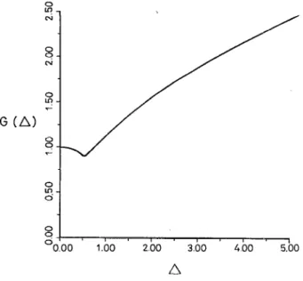
205 1.00 2.00 3.00 400 5.00 nFIG. 6. Variation of the function G(A) for the asymptotic analysis when Rn> 1.
By using Eqs. (44), (45), (46), and (47), we obtain the function gR in the limit as Rn -+ CO, and denote it by gR m . The result is gR 00 -~(2A-l)2G(A)+O(R~1’2)+O(A2), (48) gs m where G(A) =; (I ,“’ [ ( 1+2A sin a) 1’2 and gsm=r &+OW$). i--- (49)
Here, gs m denotes the function g, as Ro -+ 03, according to the stationary pipe flow model. The function G(A) is cal- culated numerically and plotted in Fig. 6. The rotation effect increases the energy dissipation substantially in the limiting case R,+ CO in general except when A < 1. Con- sider the cases studied by Alfriend3’8 and Hraster.7 The average experimental results for g by Hi-aster are about 4.35 and 5.43 times Alfriend’s theoretical results ( zgs ,) for A=1.5 and 2, respectively (see Alfriend8). Here the rotating pipe flow model using Eq. (48) predicts gRe&S,- -5.36 for A=1.5 and 13.84 for A=2, which agree much better with Hraster’s experiments in compari- son with Alfriend’s theoretical prediction using the station- ary pipe flow model.
For small Rn, gR o increases monotonically with R, , according to Eq. (39a). On the other hand, gR m decreases monotonically as R, increases for large R, [see Eq. (48)]. Hence, we expect g should attain a maximum at an inter- mediate value of Rn for a given value of A, which is similar
to the behavior of the stationary pipe flow results according to Bhuta and Koval.5 The numerical solution (see Sec. V) indeed shows this behavior and Eqs. (39a) and (48) form an envelope for the numerical result.
We have carried out the analysis for higher order so- lutions with an additional assumption that A(1 (not shown in this paper). Further assumptions are required for cases with finite A. We have not carried out such studies in the present work because of the following reasons: ( 1) Eq. (48 ) is good enough for studying the energy dissipation for cases with large R,, (2) Ro=O(lO)-O(100) for many practical situations, which can not fullfilled the asymptotic condition RR-+m, and (3) Eqs. (27a)-(27c) can be solved quite easily via numerical method in comparison with the theoretical analysis.
V. NUMERICAL SOLUTION
Detailed flow structure for R,=O( lo-‘)-0( 103) and A=O-2 have been simulated numerically by solving Eqs. (27a)-(27c) and (31a)-( 31c). Consider first the zeroth- order flow field. Equations (27a)-(27c) suggest that & is symmetric about the x’ and y’ axes, and q. is symmetric about the y’ axis but antisymmetric about the x’ axis of Fig. 5 [see Eqs. (22a) and (23a)]. Hence, we need only to consider the first quadrant of the flow field for the calcu- lations. By introducing the zeroth-order vorticity co,
g)=v27j
0,Eqs. (27a) and (27b) become
(50a)
1
i~o--V2~o=-2A azo
i aw,
4-l -sina+--cosa Jr r da (sob)
and
1
ifio-- V2Wo=2A 1 aqo w.
&l - - r da cos cr+- dr sin a (5Ocl The boundary conditions for Eqs. (50a)-(50c) are
=jo( La) -$ (1,a) =O, (51b)
and
aiij,
azo
aa (r,O) =x
=Eo( 1,a) -2A+ l=O. (51c)All the differential terms in Eqs. (50a)-( 5Oc) and (51a)- (51~) are replaced by central difference approximations, and the resulting finite difference equations constitute a complex linear algebraic system. The standard LU decom- position method for inverting a matrix is employed to solve such linear complex system of algebraic equations. It re- quires 83 CPU seconds in the CONVEX Cl computer to solve a case with 41 nonuniformly spaced grids in the r direction and 19 uniformly spaced grids in the a direction. Details of the calculation procedures and finite difference equations can be found from Ho.13
A. Grid dependence
Asymptotic analysis for R,) 1 in Sec. IV shows that the velocity gradient is large in the r direction near the wail but is small in the (r direction. Hence, we put N uniformly spaced grids in the a! direction, but employed M grids in the r direction with M, uniformly spaced grids in the core region and M-M1 nonuniformly spaced grids in the region near the wall. Let 6 be the grid spacing between the uni- formly spaced grids in the r direction. Also let (T be a factor less than unity, which is employed to specify the rate of change of the grid spacing between the nonuniformly spaced grids. In the following equation, Mt , h, and (T are
related by a
M--M,
(k+-l)&+ c B&=1, (524
i=l
which says that the grid spacing decreases from t% contin- uously toward the wall at r= 1, with the smallest grid spac- ing (h_min) next to the wall. Once M, M,, and (T are spec- ified, h can be calculated directly from Eq. (52a) as
(52b)
For the present calculations, we employed the following grid systems: (1) grid #l: M=41, Mt=41, (T=O, and N=19 (uniform grids), (2) grid #2: .M=41, M,=31, a=0.9, andN= 19, (3) grid #3: M=41, Mt=31, 0=0.8, and N=19, (4) grid #4: M=41, Mt=31, a=0.7, and N=19. The grid spacing in the a direction for all these four grid systems is 5”. According to Eqs. (52a) and (52b), z=O.O25, 0.027 885, 0.029 788, and 0.030 991, and h,,=0.025, 0.009 72, 0.0034, and 0.000 88 for grid #l, #2, #3, and #4, respectively. The variation of B is small but that of hmin is large for different grids.
Table I shows the normalized energy dissipation func- tion g for different values of Ra and A at A =O. It is found that smaller hmin is required for cases with larger values of R, . By requiring that the variation .of & be less than l%, we employ grid #4 for cases when R&a 1000, grid #3 for
cases when R,=400-700, grid #2 for cases when
Rn = 100-200, and grid # 1 for cases when R, < 100. Grid dependence test has also been carried out for different val- ues of N (i.e., the grid spacing in the a direction), and it is found that N= 19 is accurate enough for the simulations.
B. Validity of the computer program
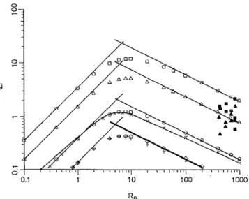
The computer program for generating the numerical results is checked by comparing with Hraster’s experimen- tal data for the energy dissipation and with the asymptotic solutions in Sec. IV for the detailed flow field. First we check against the energy dissipation. Figure. 7 shows the numerical calculations for the normalized energy dissipa- tion function g (include g’& for A+0 and g=gs for A=O) together with the asymptotic solutions in Sec. IV. Also presented in Fig. 7 are the theoretical results based on the stationary pipe flow model (Bhuta and Koval’ and Alfriend3) and Hraster’s7 experimental data. The numeri- cal results agree nicely with the asymptotic solutions for
TABLE I. The normalized energy dissipation function g for different grid systems at different values of R, and A.
R, A Grid #l Grid #2 Grid #3 Grid #4 1000 1000 1000 iom 1000 400 400 400 400 4oct 100 100 100 100 100 10 10 10 10 10 2.0 1.5 1.0 0.2 0.0 2.0 1.5 1.0 0.2 0.0 2.0 1.5 1.0 0.2 0.0 2.0 1.5 I.0 0.2 0.0 1.9703 1.9914 0.7589 0.7759 0.1544 0.1604 0.0451 0.0485 0.1268 0.1359 3.0696 3.1277 1.2050 1.2290 0.2504 0.2560 0.0740 0.0762 0.2074 0.2134 5.8727 5.9404 2.3571 2.3802 0.5073 0.5116 0.1465 0.1476 0.4089 0.4121 11.983 12.017 5.1914 5.2023 1.2294 1.2310 0.3975 0.3977 1.0966 1.0972 2.0147 2.0253 0.7844 0.7880 0.1621 0.1628 0.049 1 0.0494 0.1376 0.1386 3.1493 3.1580 1.2363 1.2390 0.2573 0.2581 0.0767 0.0769 0.2149 0.2155 5.9538 2.3855 0.5128 0.1478 0.4125
Rn( 1 when Rn< 1, and with the asymptotic solutions for R,g 1 when R&250. For A=O, the present numerical cal- culations also agree with the results based on the stationary pipe flow model for all values of Rn except when R,<l, which is due to the transient term in Alfriend’s result. Note that only the quasisteady solution is analyzed in the
9
2
0.1 1 IO 100 1000
42
BIG. 7. Variation of the normalized energy dissipation function g for different values of Rn and A when A =O. The curve shows the stationary pipe flow result by Bhuta and Koval. The straight lines with positive slopes, starting from top, are the asymptotic solutions for R,41 when A=2, 1.5, LO.8, and 0.2, respectively (the last two lines coincide to each other). The straight lines with negative sIopes, starting from top, are the asymptotic solutions for Rn, 1 when A=2, 1.5, 1, 0.8, and 0.2, iespec- tively. The numerical results are denoted by data points: “U” for A=2, “A” for A= 1.5, “0” for A= 1, “x” for A=O, “0” for A=O.8, and “+” for A=0.2 The solid squares and triangles represent the experimental results by Hraster when A=2 and 1.5, respectively.
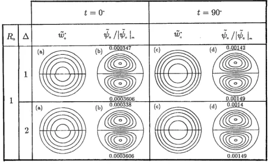
0.0003606
FIG. 8. Comparison between the-num_erical calculation (upper semicircle of each figure) and the asymptotic solution as Rn( 1 (lower semicircle) for the zeroth-order results, kY$ and &/ 1 $e 1 m, where 1 $a 1 m is the maximum value of 1 &I. The contour values, starting from the boundary, are (a) 1.00, 0.99, 0.98, 0.97, 0.96, (b) _O, 0.3 0.4, 0.6, 0.8, 0.99, (c) 0, 0.0% 0.10, 0.15, 0.20, and (d) 0, -0.2, -0.4, -0.6, -0.8, -0.99. The value next to each semicircular figure of the $a/\ +c I m contours is the value of I $e 1 m for that case.
present study, and the transient contribution to g is larger for smaller
Rn
(see Alfriend’). The numerical results also indicate that there exists a maximum value of g at R,=: 10 for a given A. The numerical results for A=0.8 and 1 coincide with those for A-0.2 and 0, respectively, for small values of Rn , which can be expected from Eq. (39a). As suggested by the asymptotic results, the numerical so- lutions also indicate that g( =gR) =0 for A=OS, g, <gs for A approximately less than unity, and gR/gs increases rapidly with A for A > 1. By comparing with Hraster’s experiments, both the asymptotic and the numerical solu- tions in the present rotating pipe flow model agree nicely with the experiments for A= 1.5, but is about two times greater than those experimental results for A=2. Recall that the experimental results are about five times greater than the theoretical prediction based on the stationary pipe flow model, gs (see Alfriend’).The normalized flow properties defined as
1 -
G&q,$) =2A- 1 (~ot~o,~oo,
will be employed to express the following numerical re- sults. Figure 8 compares the numerical solutions for R,= 1 with the asyrnptotjc solutions for Rh 4 1. Both the co_ntours for G? and W’I$OI~ are pl$ted in Fig. 8. Here 1 $e 1 m is
the maximum value of I qol. The numerical solutions (even Rn= 1 here) agree nicely with the asymptotic solu- tions for Rn Q 1. The agreement is better for smaller value of Rn . Figure 9 compares the numerical solutions with the asymptotic solutions for Rns 1 according to Eqs. (42a) and (42b), (44a)-(44c) and (45a)-(45c) at a=o” and 90”
(see Fig. 5) when Ro=lOOO. For A=O, the flow is axi- symmetric and the numerical solution agrees perfectly with
the asymptotic result for all the time, t. The agreement between the numerical and the asymptotic solutions are also nice for A#O. The numerical solution for R,=400 (not shown here) also agrees fairly with the asymptotic solution.
C. The zeroth-order flow field
As the flow studied in this paper is quasisteady, Go and q. are periodic in t with period 2~. Further Eqs. (28) show that
G&,a,t) = -i&(r,a,n-+t),
$oo(r,a,t>
= -&(r,a,r+t).
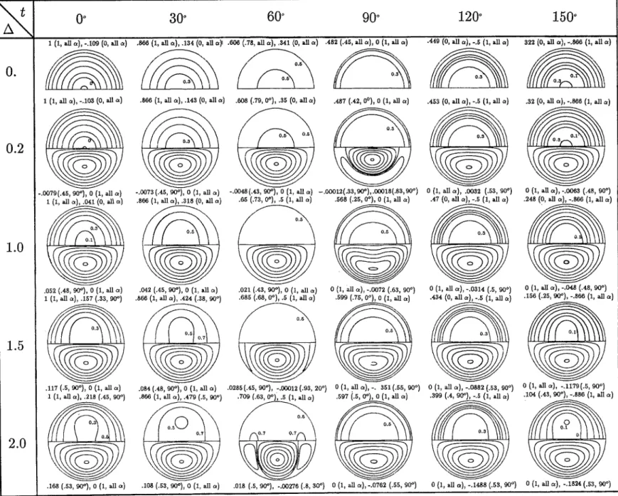
Thus the results for t=O--rr are sufficient to provide enough informations for the flow field. In this paper, we present the result at six distinct time instants; r=O”, 30”, 60”, 90”, 120“, and 150”, to show the time development of the flow field. The results at t= 180” are the same as those at t=O” except the signs are changed. Many cases have been simulated and some of the typical cases are reported here. Figures 10-12 show the contours for the normalized axial velosity ij$ and the normalized secondary stream- function &/I go I m for different A’s at Rn= 10, 100, and
1000, respectively. Since the axial (primary) and the sec- ondary flow are symmetric and antisymmetric, respec- tively, with respect to the x’ axis in Fig. 5 [see Eq. (22a)], we pl_ot zi?: in the upper semicircle (r=O- 1, a=O--rr) and WIti~l~ in the lower semicircle (r=O-1, a=v
-2~) together in order to provide a more clear picture to illustrate the intera_ctioft between the primary and the sec- ondary flow. The $+,/I r/e I m contours in the upper semicir-
2420 Phys. Fluids A, Vol. 5, No. 10, October 1993 U. Lei and C. F. Ho
e:
B
cm
-3
8
3
.‘a
1
a-
b)
!
$
8
$
6
73
B
%
g
1
&
2
-cl
3
98
3
2
2
3
i
s
3
-2
2
G
22
8
2
P
2
s
g
Q
B
P
2
6
.B
B
d
s
2
c
2
3
2
i ‘t
s
z
3
a
f
&
.a
8
2
i-i
ga
2
;i!
E F
24203
Y
9
I!
E.
z:
P
6
r
cn
5
-2
g
8
e
G
8
0
0
a
120
1506
1 (1, dl a), -.lO?l (0, au a) .6+jf3 (1, all Q), .134 (0, au a) A06 1.78, au a), ,341 (0, all CY) .482 (.45, all cz), 0 (1, au a)
0.
(A, (&? A.
1 (1, all a), -.103 (0, all P)
.052 (.48, W), 0 (1, all a) 1 (1, au a)> ,157 (.33, 9V)
.168 (53, 90a), 0 (1, all a)
.866 (1, all a), .143 (0, all a) .866 (1, all a), .143 (0, all a)
- -.w73 (.45, W), 0 (1, all 0) -.w73 (.45, W), 0 (1, all 0) .866 (1, all cz), .318 (0, all a) .866 (1, all cz), .318 (0, all a) .042 (.45, .042 (.45, W), 0 (1, all 0) W), 0 (1, all 0) .866 (1, all Q), ,424 (.38, 90") .866 (1, all Q), ,424 (.38, 90") .084 (.48, 9Q"), 0 (1, all CZ) .084 (.48, 9Q"), 0 (1, all a) .36e (1, all a), .479 (.5, 900) .36e (1, au a), .479 (.5, 900) do3 (.79, (P), 35 (0, all a) -.0048(.43, W), 0 (1, all a) -,. .65 (.73, a), .5 (1, all a) .021 (.43, wq, 0 (1, all CY) .636 (.6X$ O'), .5 (1, alI a) .018 (.5, 900), -.OQ276 (A, 30')
,467 (AZ, oq, 0 (1, all a)
0 (1, ~41 0): -JO72 (.63, 90*) .599 (.76, oq, 0 (1, all a)
0 (1, all a), ~0762 (.55, 90“)
.453 (0, all a), -.5 (1, all Q)
0 (1, da), -043 (.48, 90') .166 (.25, 90.'), -.866 (1, da)
0 (1, dl a), -.1824 (.53, W)
FIG. 10. Numerical solution for Et (upper semicircle of each figure) and qoo/l & I ,,, (1 ower semicircle) at Rn= 10, where I &, 1 m is the maximum value of I $a 1. The &J’ I $e I m contours in the upper s@c&cle are the same as those in the lower semicircle except that the sign is changed. The contour values for i3;T are - 1, -0.866, -0.7, -0.5, -0.3, -0.1,0,0.1,0.3,0.5,0.7,0.866,and l.Thecontourvaluesfor1Wi~l, are -0.99, -0.8, -0.6, -0.4, -0.2, -0.05, 0, 0.05,0.2,0.4,0.6, 0.8, and 0.99. Some of the contour values are omitted for clarity. The omitted contour values can be identilied by using the rest labeled contours, and the maximum and minimum values of i? and $* together with their locations in the first quadrant (inside the parentheses) listed next to each semicircular figure. Note that there is no secondary flow for