控制系統之性能評估與線上監控(3/3)

行政院國家科學委員會專題研究計畫 成果報告

控制系統之性能評估與線上監控(3/3)

中 華 民 國 94 年 12 月 12 日

摘 要

Abstract

A systematic procedure for performance assessment and PI/PID controller design based on modified relay feedback test is proposed. The gain and phase margins of a control system are used to assess its performance. The proposed method estimates the gain and phase margins on-line by a modified relay feedback scheme, where a delay element is embedded between the relay and controller. The estimated results are used to access the goodness of the controller parameters. When the retuning of controller is found necessary, a similar procedure can be applied to tune the PI/PID controller based on specifications of gain and phase margins. Thus, performance assessment and controller improvement can be done simultaneously, which ensures the system to have good performance in control.

Keywords: performance assessment, controller design, gain margin, phase margin, relay

Contents (目錄)

1. Introduction

2. Modified Relay Feedback Structure

3. Performance Assessment

3.1 Estimation of gain margin 3.2 Estimation of phase margin 3.3 Assessment of performance

4. Controller Tuning

4.1 Tuning of PI controller 4.2 Tuning of PID controller

4.3 Specification of gain and phase margins

5. Extension to Multi-loop Systems

6. Simulation Examples

7. Conclusions

References

1. Introduction

The proportional-integral-derivative (PID) controller is widely used in chemical process industries because of its simple structure and robustness to the modeling error. Despite the fact that numerous PI/PID tuning methods have been provided in the literature, many control loops are still found to perform poorly.1 Therefore, regular performance assessment and controller retuning are necessary. In process control, minimum variance has been used as a benchmark for assessing the closed-loop performance for decades.2 This criterion is a valuable measurement of the system performance. But, focusing on the error statistics only does not meet the traditional performance requirements of PID control in chemical plants, and the system robustness was not considered directly.

Gain and phase margins have served as important measure of robustness for the single-input-single-output (SISO) system. It is also known from classical control theory that the phase margin is related to the damping of the system and thus can also serve as a performance measure. For the multi-loop control of multi-input-multi-output (MIMO) system, gain and phase margins can also be defined in the similar spirit as SISO system based on the effective open-loop process (EOP).3 Traditionally, under the assumption that the process model and controller parameters are known, the gain and phase margins are obtained by solving nonlinear equations numerically or graphically by trial-and-error use of Bode’ plots. Because calculation of gain and phase margins in such ways is very tedious, Ho et al.4,5 derived approximate analytical formulas to compute gain and phase margins of PI/PID control systems using first-order plus dead-time (FOPDT) process model. However, the assumption is not practical because the process model and controller settings may be unknown at the stage of performing the performance assessment. Thus, it is desirable to find a procedure for on-line monitoring of gain and phase margins. Recently, Ma and Zhu6 proposed a performance assessment procedure for SISO system based on modified relay feedback. Gain and phase margins are estimated by two relay tests where an ideal relay is used for the first test and a relay with hysteresis is used for the other. Due to a linear assumption about the amplitude of the limit cycle, their method may not give accurate results for processes with more complex dynamics such as process with right-half-plane (RHP) zero and oscillatory modes.

Controller designs to satisfy gain and phase margin specifications are well accepted in practice for classical control. To be free of tedious modelling and computation procedures aforementioned, Åström and Hägglund7 used relay feedback for automatic tuning of PID controllers with specification on either gain margin or phase margin, but it cannot achieve both specifications simultaneously. Some approximate analytical PI/PID tuning formulas have been derived to achieve the specified gain and phase margins.8,9 Most of them use simplified models such as FOPDT model and second-order plus dead-time (SOPDT) model. For processes with more complicated dynamics, the resulting control systems may not achieve user-specified gain and phase margins exactly. Ho et al.10 extended the work of Ho et al.8 for tuning of multiloop PID controllers based on gain and phase margin specifications.

In this paper, an on-line performance assessment procedure based on modified relay feedback test is proposed. This modified relay feedback structure embeds an additional delay between the relay and controller. The gain and phase margins are used to assess the performance and robustness of the control systems. The proposed method can on-line estimate the gain and phase margins for systems with both unknown controller parameters and process dynamics. For multi-loop systems, the modified relay tests are conducted in a sequential manner to estimate the gain and phase margins of each loop. The estimated results can be used to indicate the appropriateness of the controller parameters. When the retuning of controller is found necessary, a similar procedure can be applied to tune the PI/PID controller based on the user-specified gain and phase margins, where process models are not required. In this way, performance assessment and controller re-tune can be done simultaneously, which ensures a good performance of the control system.

This paper is organized as follows. Section 2 describes the proposed modified relay feedback structure. On-line procedures for performance assessment and controller design are presented in Section 3 and 4, respectively. Section 5 extends the methods to multi-loop control systems. Simulation examples follow in Section 6 to demonstrate the procedures and effectiveness of the proposed methods. Conclusions are drawn in Section 7.

2. Modified Relay Feedback Structure

Åström and Hägglund.7

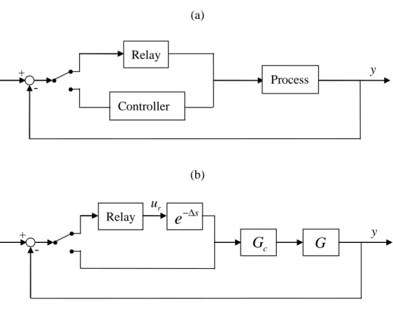
The block diagram of the standard relay feedback system is as shown in Figure 1(a). The system generates a continues cycling if it has a phase lag of at least π . A limit cycle with a period P results and this period is the ultimate period. u

Therefore, the ultimate frequency from this relay feedback test is: 2 u u P π ω = (1)

From the describing function approximation, the ultimate gain can be approximately given by: 4 u h K a π = (2)

where h is the relay output magnitude and a is the amplitude of limit cycle. In other words, one point, i.e. the critical point, on the Nyquist curve of the process can be obtained from relay feedback test.

For the purpose of performance assessment, a modified relay feedback structure is proposed as shown in Figure 1(b) where G , _c G, u , and y are the controller, process, _r

relay output, and process output, respectively. Moreover, a delay element, e−∆s, is embedded between the relay and the controller. Compared with the conventional relay feedback, the most important features of this modified structure are that the controller is always connected in line with the process and an additional delay is embedded. Due to the first feature, the lump frequency information of process and controller, which is required for performance assessment, can be obtained while only process information is extracted in the conventional relay feedback test. Besides, the inserted additional delay is used to obtain other points (except critical point) on the Nyquist curve which are helpful for the estimation of phase margin. The insertion of additional delay has also been used in conventional relay feedback for process identification11 and other points on the Nyquist curve can also be obtained by inserting other elements or using a relay with hysteresis6,7,12. This proposed structure can ensure the existence of limit cycle even for a low-order process without time delay. As a result, it can assess the performance of the closed-loop system by on-line estimation of gain and phase margins, as presented in the following section, to determine if a retuning of the controller is necessary.

3. Performance Assessment

As has been mentioned, gain and phase margins are good measurements for the performance and robustness of control systems. However, without any information about the controller and process, it is impossible to calculate the gain and phase margins by solving equations analytically, numerically, or graphically. In this section, a systematic procedure that can on-line estimate gain and phase margins of a completely unknown system by the proposed modified relay feedback test is presented to assess the performance of the control system.

3.1 Estimation of gain margin

Consider the modified relay feedback system as shown in Figure 1(b). For the estimation of gain margin, by setting ∆ as zero, the frequency known as phase crossover frequency, ω , that has a phase lag π is required. Let the loop transfer function be _p

( ) ( ) ( )

LP c

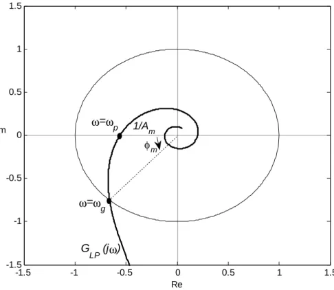
G s =G s G s . The system starts to oscillate and then attain a limit cycle. The oscillating point is the intersection of the Nyquist curve of G_LP( )s and the negative real

axis in the complex plane, as shown in Figure 2. The phase crossover frequency of ( )

LP

G s can be calculated by Eq.(1) as ω_p =2π P_p, where P is the period of the limit _p

cycle. In addition, using the approximation of describing function, the amplitude of

( )

LP

G s can be calculated by Eq.(2) as GLP

( )

more accurate estimation, GLP

( )

14,15

( )

∫

∫

Therefore, the gain margin, A , can be estimated as: _m

( )

3.2 Estimation of phase margin

When the estimation of gain margin is finished, the delay ∆ is then set as a non-zero value in order to extract the frequency information of G_LP( )s at some

frequency other than ω for the estimation of phase margin. With a given value of _p ∆, assume that the system oscillates with a period of P and then we have the phase of the system as:

( )

{

}

{

( )

}

where ω=2π P. To calculate the phase margin, the desired frequency is the gain crossover frequency, ω , of g GLP( )s , which is the intersection of the Nyquist curve of

( )

LP

G s and the unit circle in the complex plane, as shown in Figure 2. Denote the desired

value of ∆ that make the amplitude of G_LP

( )

phase crossover frequency of GLP

( )

. In this case, Eq.(5) can be written as

( )

{

}

arg G_LP jω_g − ∆_dω_g = −π where ω_g =2π P_g . Then, it follows that the phase margin,

m

φ , can be estimated as:

( )

{

}

arg

m GLP j g d g

φ = ω + = ∆π ω (6)

To find the value of ∆_d, an on-line iterative procedure as the following is presented. Starting from an initial guess ∆( )0 , the value of ∆ is updated by

( )1 ( ) ( )

(

(

)

)

where γ( )i >0 is the convergence rate and G_LP

(

)

(

)

(

)

∫

∫

Notice that we have ∆ =_d 0 if A_m =1, and, in general, ∆_d increases as A and _m P _p

chosen as:

(

)

(

)

which make Eq.(7) have a quadratic convergence rate near the solution.7 In each iteration, the value of ∆( )i holds constant until the output generates two or three oscillating cycles and then switches to the next value in an on-line adaptive way. When Eq.(7) converges, the resulting value of ∆ is taken as ∆_d.

3.3 Assessment of performance

With the estimated gain and phase margins, the robustness of the current system can be assessed. The recommended ranges of gain and phase margins are between 2 and 5 and between 30o and 60o. Nevertheless, gain and phase margins indeed are closely related to the time-domain performance of the system.

For set-point tracking, a control system with gain margin 2.1 and phase margin 60o can have the optimal integral of the absolute value of the error (IAE).16 The corresponding loop transfer function is as the following form:

(

)

where θ is the apparent dead-time of the process. For inverse-based controller design, such as internal model control (IMC) design, the loop transfer function has the following form: ( ) s LP k e G s s θ − = (11)

where k is a user-specified parameter to make trade-off between speed of response and robustness of the closed-loop system. The gain and phase margins of the resulting closed-loop system satisfy the following relation:

1 1 2 m m A π φ = _ − _   (12)

It is well-known that the inverse-based design can give good set-point response. Moreover, the system has optimal IAE value for set-point change if the value of k is chosen as

0.59

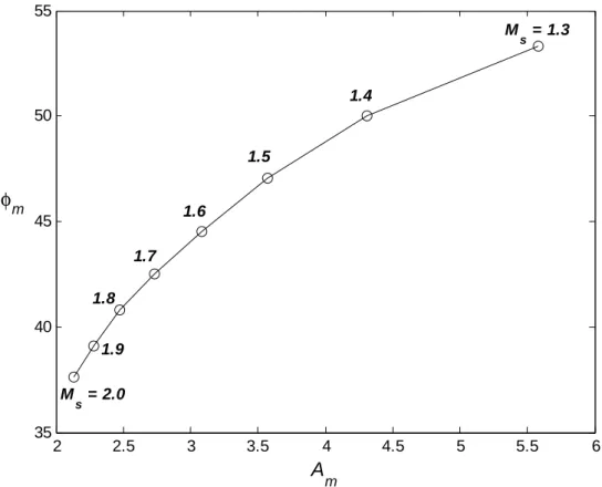
satisfied by the estimated gain and phase margins, the set-point performance is not satisfactory. On the other hand, the inverse-based design also gives good disturbance response for dead-time-dominate processes, but results in sluggish disturbance response for lag-dominate processes.17 In the case of lag-dominate process, if good disturbance response is desirable, the gain and phase margin pair

(

)

Ms which is the maximum of the magnitude of the sensitivity function, 1 1

(

( )

)

(

)

performance may be poor. Therefore, based on the gain and phase margins, not only the system robustness, but also the possibility of achieving good control performance can be assessed.

4. Controller Tuning

After assessment, when the performance of the control system is found poor, retuning of the controller is needed. The modified relay feedback scheme can be applied for on-line tuning of PI/PID controller to achieve user-specified gain and phase margins, designated as A and *_m φ , respectively. By this way, neither intermediate process model nor _m*

nonlinear equations solving is required.

4.1 Tuning of PI controller

Consider the PI controller of the following transfer function. 1 ( ) 1 c c I G s k s τ   = _ + _   (13)

For a given value of ∆, the parameters, k and _c τ , can be found to satisfy the _I

specification of phase margin. In other words, they can be found such that the following two equations hold.

* * 2 or m g g m P π φ ω φ ∆ = ∆ = (14)

( )

( )

∫

∫

By the modified relay feedback test, Eq.(14) can be satisfied by adjusting the value of τ _I and then Eq.(15) can be satisfied by adjusting the value of k . However, the specification _c

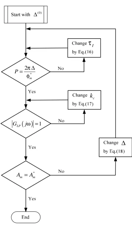
of gain margin may not be necessarily achieved by such obtained controller parameters. In general, the gain margin of the resulting system aforementioned, i.e. system with φ_m =φ_m*, is a function of ∆ value. Therefore, there exists a certain value of ∆ which can make the gain margin of the resulting system meet its specification. According to the analysis, an iterative procedure for tuning the PI controller using the modified relay feedback test is presented as follows:

1) Starting with a guessed value of ∆, i.e. ∆(0) . 2) Adjust τ by the following equation: I

( 1) ( ) ( ) ( ) 1 * 2 i i i i I I m P π τ τ γ φ + _{= −}  ₋ ∆     (16)

where P is the period of limit cycle in the i-th iteration. Eq.(14) holds when Eq.(16) ( )i

converges.

3) Adjust k by the following equation until it converges so that Eq.(15) holds, _c

(

)

(

)

where ω( )i =2π P( )i and GLP

(

)

4) Set ∆ =0 and estimate A by Eq.(4). _m

5) Check if the estimated A equals _m A . If not, change the value of _m* ∆ by the following equation and go back to step 2) until A_m= A*_m holds.

(

)

The convergence rates, γ , ₁( )i γ and ₂( )i γ , can be defined in the similar manner of Eq.(9) ₃( )i as: ( ) ( 1) ( ) 1 ( ) ( 1) i i i I I i i P P τ τ γ = − −₋ − (19)

(

)

(

)

Notice that γ₁( )i <0, γ₂( )i >0 and γ₃( )i >0. For FOPDT process, inserting a delay ∆ in the relay feedback loop results in an increase of approximately 4∆ in the period of limit cycle. In order to improve the convergence of Eq.(16), it is desirable that

(

)

*

2π φ∆ _m= ≈P P_p + ∆4 . Thus, the initial guess of ∆ is suggested as:

(0) * 2 4 p m P π φ ∆ = − (22)

This design procedure is shown graphically in Figure 4.

The procedure is performed in an on-line adaptive manner. In each of the iterations, two or three oscillating cycles are generated from modified relay feedback test to compute the required quantities for the next iteration. When the value of ∆ converges, the resulting controller parameters are the desired ones which can make the control system achieve both user-specified gain and phase margins.

4.2 Tuning of PID controller

For the tuning of PID controller, a similar procedure can be applied. The PID controller transfer function is given as:

1 ( ) 1 c c D I G s k s s τ τ   = _ + + _   (23)

Since there is one more parameter to be tuned, an additional condition must be introduced to determine the parameters uniquely. The derivative time, τ , is usually chosen as a _D fixed ratio of the integral time, τ , as: _I

D I

τ =ατ (24)

Researchers7,18 have recommended that α =0.25. With the relation of Eq.(24), the procedure for PI controller tuning presented in the previous section can be applied directly to tune the PID controller.

If τ is not chosen as a fixed ratio to _D τ , then the extra degree of freedom can be _I used for achieving another performance requirement. For example, Zhuang and Atherton19 discuss the tuning of PID controller to achieve optimal integral time-weighted square error (ITSE) performance criterion and suggest the value of α as:

0.413 3.302 1 α κ = + (25)

where κ is the process-normalized gain defined by κ = G j

( ) ( )

Eq.(25), the steady-state gain and ultimate gain of the process are required. These information can be estimated from the modified relay feedback test by setting ∆ =0,

1

c

k = , τ_D =0, and τ as a very large value. In fact, such setting restores the modified _I relay feedback to the conventional relay feedback scheme. Of course, this is at the cost of extra experiment.

4.3 Specification of gain and phase margins

There are some restrictions on the specification of the gain and phase margin pairs. One usual requirement is that the controller parameters have to be positive. Ho et al.8 have provided the feasible region of gain and phase margin specifications for PI and PID control based on FOPDT and SOPDT process models, respectively. But the region depends on the parameters of the model. Generally speaking, if a larger gain margin is specified, a higher value of phase margin should also be specified accordingly.

In order to achieve better performance, the specification of

(

)

consider the control objective. As bas been mentioned in Section 3.3, for set-point tracking, it is suitable to specify

(

)

(

)

for lag-dominate processes.

5. Extension to Multi-loop Systems

Multi-loop SISO controllers are often used to control chemical plants which have MIMO dynamics. Ho et al.10 defined the gain and phase margins based on the Gershgorin

bands of the multi-loop system. However, according to their definition, the gain and phase margins of each one loop are independent of the controllers in the other loops so that the interactions between loops are not considered. In this paper, the gain and phase margins are defined in the similar spirit as SISO system based on the effective open-loop process (EOP) in the work of Huang et al.3. The i-th EOP describes the effective transmission from the i-th input to the i-th output when all other loops are closed. With the formulation of EOP, the multi-loop control system can be considered as several equivalent SISO loops.

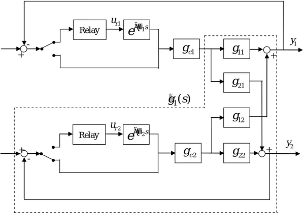
Consider the multi-loop control system of a 2x2 multivariable process with the following process and controller transfer function matrices, G( )s and G_C( )s .

11 12 21 22 ( ) ( ) ( ) ( ) ( ) g s g s s g s g s   =     G (26) 1 2 ( ) 0 ( ) 0 ( ) c c g s s g s   =     C G (27)

The mathematical definition of the two EOPs, g s%₁( ) and g s%₂( ), are given as:3

[

]

[

]

Based on the EOPs of Eq.(28), the loop transfer functions of the equivalent loops are

,1( ) 1( ) 1( )

LP c

G s =g s g s% and G_LP,2( )s =g_c2( )s g s%₂( ). Therefore, as the case of SISO system, the gain and phase margins of each loop can be estimated by sequentially using of the proposed modified relay feedback system. Figure 5 shows the modified relay feedback scheme for the estimation of gain and phase margins of the first loop, where loop 1 is under relay mode and loop 2 is under control mode. Then, the modes of loops are switched to estimate the gain and phase margins of the second loop. This procedure can be extended to a general multi-loop system, where the modified relay tests are conducted in a sequential manner to estimate the gain and phase margins of each loop. Since the

mathematical formulation of EOPs for high-dimensional processes is complex, calculation of gain and phase margins from process models in the traditional way becomes very difficult. However, the proposed procedure can be easily applied in high-dimensional

processes regardless the complexity of the EOPs.

When retuning of the controller is found necessary, a similar procedure like the case of SISO system can be applied to tune the controller gci( )s to meet the specification of gain and phase margins of the i-th loop. If gain and phase margins of more than one loop are simultaneously specified, the controller tuning needs to go through an iterative procedures due to the interaction nature of multi-loop system. In that case, gain and phase margins should be carefully specified to ensure the convergence of the controller parameters.

6. Simulation Examples

Example 1.

Consider a control system with FOPDT process and PI controller given by: 1 ( ) , ( ) 0.616 1 1 0.765 s c e G s G s s s θ − _{ } = = _ + _ +  

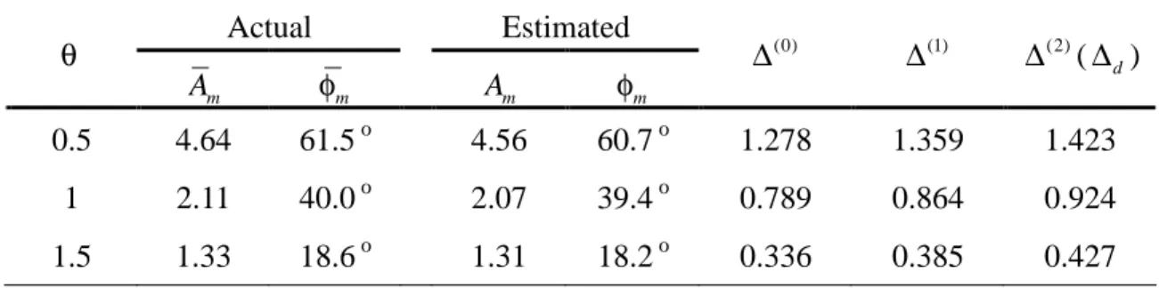
Three different values of the dead-time, θ =0.5, 1, 1.5, are used for simulation. As shown in Table 1, the actual gain and phase margins, designated as A and _m φ , for these three _m

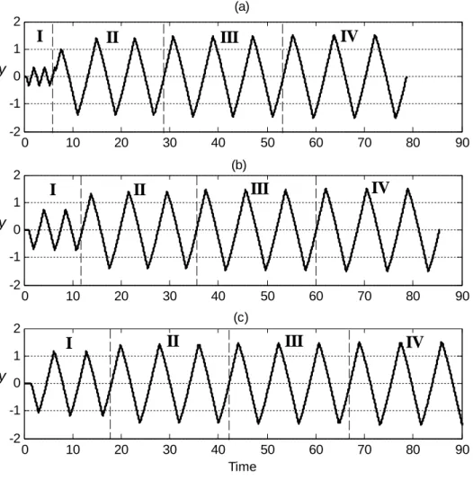
cases cover a wide range. Based on the proposed relay feedback test, the estimated gain and phase margins together with the values of ∆( )i during iteration are also shown in Table 1 for comparison. The value of ∆ converges after two iterations. It can be seen from Table 1 that the estimated gain and phase margins are very close to the actual ones. The output responses during the estimation procedure are shown in Figure 6, where period I is for estimating gain margin and periods II to IV are for estimating phase margin.

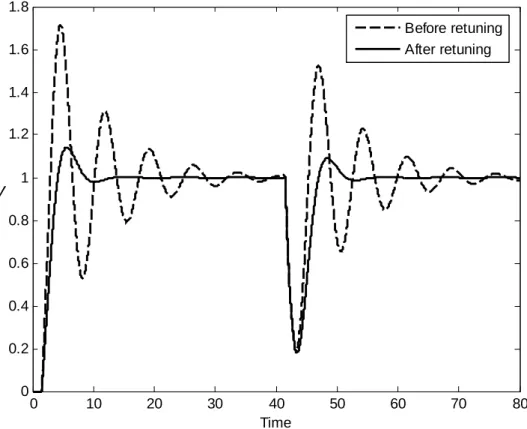
For the case of θ =1.5, because the gain and phase margins of the control system (1.31 and 18.2 o) are quite away from the recommended ranges, the performance and robustness are poor. Thus, retuning of the controller is needed. We specify the gain margin as A_m* =2.5, and then the phase margin is specified according to Eq.(12) as φ_m* =54o. This design is equivalent to the IMC design so that the control system is expected to have good set-point response. The tuning procedure is shown in Table 2. The results converge after two iterations of ∆ (∆ =(2) 2.239), and the PI controller is obtained as:

1 ( ) 0.424 1 1.008 c G s s   = _ + _  

The actual gain and phase margins of this resulting control system are A_m=2.49 and o

53.2

m

φ = , which are very close to the specified ones. The closed-loop responses before and after retuning are shown in Figure 7, where the performance is significantly improved after controller retuning.

Example 2.

Consider a second order process and a PID controller given by:

(

)(

)

The actual gain and phase margins are 2.63 and 56.5o, respectively. Based on the modified relay feedback, the estimated gain and phase margins are A_m=2.62 and φ_m =56.1o, where the value of ∆ converges after two iterations with ∆ =(0) 1.089, ∆ =(1) 1.298 and

(2)

1.655

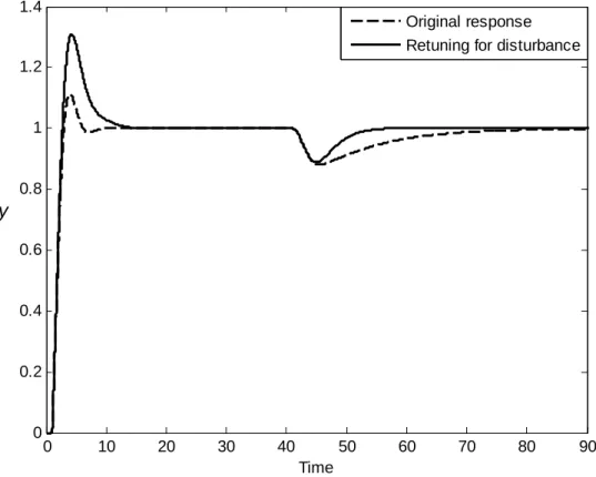
∆ = . According to the estimated result, this control system is expected to have good set-point response but sluggish disturbance response because the

(

)

Better disturbance response can be achieved if we retune the PID controller based on specifications given in Figure 3. By choosing M_s =1.8, the specifications are found as

* 2.5

m

A = and φm* =41o. The value of α in Eq.(24) is chosen as 0.25. The tuning procedure converges after one iteration of ∆ ( (1)

1.198

∆ = ), and the PID controller is obtained as: 1 ( ) 8.255 1 1.409 5.634 c G s s s   = _ + + _  

The actual gain and phase margins of this resulting control system are A_m=2.54 and o

42.8

m

φ = . The closed-loop response after retuning is also shown in Figure 8, where the disturbance response is much improved. However, the set-point response becomes not so satisfactory due to the control objective we designed for. This result indicates that the gain and phase margins are indeed related to the control performance so that the control objective should be taken into account when the controller is tuned to achieve user-specified gain and phase margins.

Example 3.

Consider a high-order process and a PID controller given by:

(

)

The actual gain and phase margins are 1.70 and 23.8o, respectively. Based on the modified relay feedback, the estimated gain and phase margins are A_m =1.66 and φ_m=22.7o, where the value of ∆ converges after two iterations with ∆ =(0) 0.820, ∆ =(1) 0.726 and ∆ =(2) 0.663.

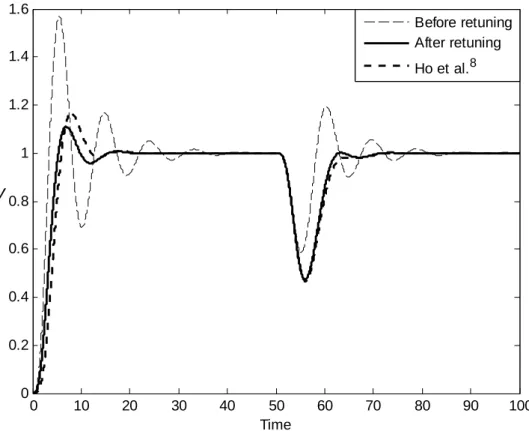
To improve the system performance, retune the PID controller according to the specifications of A_m* =3 and φ_m* =60o. Again, the value of α in Eq.(24) is chosen as 0.25. The results converge after two iterations of ∆ (∆ =(2) 2.999), and the PID controller is obtained as:

1 ( ) 1.207 1 0.913 3.651 c G s s s   = _ + + _  

The actual gain and phase margins of this resulting control system are A_m=3.04 and o

59.1

m

φ = , which are very close to the specified ones. For this process and the same specifications, the PID controller tuning proposed by Ho et al.8 results in A_m=3.38 and

o 62.5

m

φ = . Our proposed method can achieve the specifications more closely. The closed-loop responses before retuning, after retuning and by Ho et al.8 are shown in Figure 9. The proposed controller also has better performance than that of Ho et al.8.

Example 4

Consider a process with RHP zero and a PI controller, which are used for simulation in Ma and Zhu6, given by:

(

)

(

)

For the cases of β =1 and β =0.1, the actual gain and phase margins together with the estimated values by Ma and Zhu6 and the proposed method are given in Table 3 for comparison. It is seen from Table 3 that the proposed method can estimate the gain and phase margins more accurately than the method proposed by Ma and Zhu6. The error between actual and estimated phase margin by Ma and Zhu6 is large for processes with RHP zero.

For the case of β =1, the gain and phase margins of the control system are too small to have reasonable performance. Thus, the PI controller is retuned by the proposed procedure with the specifications chosen as A_m* =3 and φ_m* =60o. These specifications are achieved after two iterations of ∆ (∆ =(2) 4.961), and the PI controller is obtained as:

1 ( ) 0.32 1 1.524 c G s s   = _ + _  

The actual gain and phase margins of this resulting control system are A_m=3.22 and o

60.3

m

φ = . The closed-loop responses before and after retuning are shown in Figure 10.

Example 5.

Consider a 2x2 Wood and Berry process given by:

3 7 3 12.8 18.9 16.7 1 21 1 ( ) 6.6 19.4 10.9 1 14.4 1 s s s s e e s s s e e s s − − − −  −   _{+ +}    = −    _{+ +}    G

The performance of multi-loop PI controllers proposed by Loh et al.20 as the following is assessed. 1 2 1 1 ( ) 0.868 1 , ( ) 0.087 1 3.25 10.4 c c g s g s s s     = _ + _ = − _ + _    

The actual gain and phase margins calculated are given in Table 4. The modified relay feedback tests are conducted sequentially to estimate the gain and phase margins of two equivalent SISO loops. The procedure and estimated results are shown in Table 4. The numbers of iteration for the first and second loops are 2 and 4, respectively. The estimated values are close to the calculated ones, which indicates the proposed method is also effective for multi-loop control systems. The set-point responses of this system are shown in Figure 11. The response of loop 1 is aggressive due to its lower gain and phase margins. However, the response of loop 2 is sluggish because its phase margin is very large.

To improve the control performance, retune g_c2( )s first by specifying A_m*_,2 =2.2 and φ_m*_,2 =70o for the second loop. The result converges after two iterations of ∆₂ (∆ =(2)₂ 10.49), and g_c2( )s is obtained as:

2 1 ( ) 0.076 1 5.24 c g s s   = − _ + _  

The actual gain and phase margins of this resulting control system are A_m,1=2.07 and o

,1 32.6

m

φ = for loop l, and A_m,2 =2.21 and φ_m,2 =71.8o for loop 2. The gain and phase margins of loop 2 are very close to the specified ones after retuning, while the gain and phase margins of loop 1 are similar to those before retuning. Then, retune g_c1( )s by

specifying A_m*_,1=2.5 and φ_m*_,1 =50o for the first loop. The result converges after one iteration of ∆₁ (∆ =₁(1) 1.76), and g_c1( )s is obtained as:

1 1 ( ) 0.771 1 7.17 c g s s   = _ + _  

Now, the actual gain and phase margins after retuning of two controllers are A_m,1 =2.49 and φm,1=53.2o for loop l, and Am,2 =2.33 and

o ,2 73.1

m

φ = for loop 2. They are close to the specified ones. The closed-loop responses after retuning are shown in Figure 11. It is seen that the performance of loop 2 is improved after retuning of g_c2( )s , and the

performance of loop 1 is improved after retuning of gc1( )s .

7. Conclusions

A systematic procedure for performance assessment and PI/PID controller design

based on modified relay feedback test is proposed in this paper. The proposed method can on-line estimate the gain and phase margins for systems with both unknown controller parameters and process dynamics. The estimated results can be used to assess the performance of the closed-loop system. When the retuning of controller is found necessary, a similar procedure can be on-line applied to tune the PI/PID controller based on the user-specified gain and phase margins. Simulation results have shown that the proposed method is effective for processes with different kinds of dynamics and for multi-loop systems. Performance assessment and controller design can be done simultaneously, which can ensure a good performance of the control system.

References

(1) Ender, D. B. Process Control Performance: Not as Good as You Think. Control Eng.,

1993, 40, 180.

(2) Harris, T. J.; Seppala, C. T.; Desborough, L. D. A Review of Performance Monitoring and Assessment Techniques for Univariate and Multivariate Control Systems. J.

Process Control, 1999, 9, 1.

(3) Huang, H. P.; Jeng, J. C.; Chiang, C. H.; Pan, W. A Direct Method for Multi-loop PI/PID Controller Design. J. Process Control, 2003, 13, 769.

(4) Ho, W. K.; Hang, C. C.; Zhou, J. H. Performance and Gain and Phase Margins of Well-Known PI Tuning Formulas. IEEE trans. Control Syst. Technol., 1995, 3, 245. (5) Ho, W. K.; Gan, O. P.; Tay, E. B.; Ang, E. L. Performance and Gain and Phase

Margins of Well-Known PID Tuning Formulas. IEEE trans. Control Syst. Technol.,

1996, 4, 473.

(6) Ma, M. D.; Zhu, X. J. Performance Assessment and Controller Design Based on Modified Relay Feedback. Ind. Eng. Chem. Res., 2005, 44, 3538.

(7) Åström, K. J.; Hägglund, T. Automatic Tuning of Simple Regulators with Specifications on Phase and Amplitude Margins. Automatica, 1984, 20, 645.

(8) Ho, W. K.; Hang, C. C.; Cao, L. S. Tuning of PID Controllers Based on Gain and Phase Margin Specifications, Automatica, 1995, 31, 497.

(9) Wang, Y. G.; Shao, H. H. PID Autotuner Based on Gain- and Phase-Margin Specifications. Ind. Eng. Chem. Res., 1999, 38, 3007.

(10) Ho, W. K.; Lee, T. H.; Gan, O. P. Tuning of Multiloop Proportional-Integral-Derivative Controllers Based on Gain and Phase Margin Specifications. Ind. Eng. Chem. Res., 1997, 36, 2231.

(11) Scali, C.; Marchetti, G.; Semino, D. Relay with Additional Delay for Identification and Autotuning of Completely Unknown Processes. Ind. Eng. Chem. Res., 1999, 38, 1987.

(12) Chiang, R. C.; Yu, C. C. Monitoring Procedure for Intelligent Control: On-Line Identification of Maximum Closed Loop Log Modulus. Ind. Eng. Chem. Res., 1993,

32, 90.

Eng. Chem. Res., 1991, 30, 1530.

(14) Wang, Q. G.; Hang, C. C.; Zou, B. Low-Order Modeling from Relay Feedback. Ind.

Eng. Chem. Res., 1997, 36, 375.

(15) Huang, H. P.; Jeng, J. C.; Luo, K. Y. Auto-Tune System Using Single-Run Relay Feedback Test and Model-Based Controller Design. J. Process Control, 2005, 15, 713.

(16) Huang, H. P.; Jeng, J. C. Monitoring and Assessment of Control Performance for Single Loop Systems. Ind. Eng. Chem. Res., 2002, 41, 1297.

(17) Hang, C. C.; Ho, W. K.; Cao, L. S. A Comparison of Two Design Methods for PID Controllers. ISA Trans., 1994, 33, 147.

(18) Hang, C. C.; Åström, K. J.; Ho, W. K. Refinements of the Ziegler-Nichols Tuning Formula. IEE Proc. D – Control Theory and Applications, 1991, 138, 111.

(19) Zhuang, M.; Atherton, D. P. Automatic Tuning of Optimum PID Controllers. IEE

Proc. D – Control Theory and Applications, 1993, 140, 216.

(20) Loh, A. P.; Hang, C. C.; Quek, C. X.; Vasnani, V. U. Autotuning of Multiloop Proportional-Integral Controllers Using Relay Feedback. Ind. Eng. Chem. Res., 1993,

Table 1 Actual and estimated gain margin, phase margin in example 1 Actual Estimated θ m A φ _m A _m φ _m (0) ∆ ∆(1) ∆(2) (∆_d) 0.5 4.64 61.5 o 4.56 60.7 o 1.278 1.359 1.423 1 2.11 40.0 o 2.07 39.4 o 0.789 0.864 0.924 1.5 1.33 18.6 o 1.31 18.2 o 0.336 0.385 0.427

Table 2 Design procedure of PI controller in example 1 (θ =1.5)

Iteration No. i ∆ τ _I k _c A _m

0 2.494 0.834 0.321 2.74

1 2.372 0.917 0.368 2.63

2 2.239 1.008 0.424 2.49

Table 3 Actual and estimated gain margin, phase margin in example 4 Actual value Estimated6 Estimated (proposed method)

β m A φ m A m φ m A m φ m (2) d ∆ = ∆ 1 1.28 20.0 o 1.19 12.7 o 1.20 16.5 o 0.501 0.1 3.49 51.6 o 3.29 41.8 o 3.34 51.8 o 1.789

Table 4 Actual and estimated gain margin, phase margin in example 5

Actual Estimated loop m A φ _m A _m φ _m (0) ∆ ∆(1) ∆(2) ∆(3) ∆(4) 1 2.07 33.5 o 2.06 30.2 o 0.785 0.752 0.690 2 2.18 89.9 o 2.19 89.8 o 2.659 3.102 24.69 15.69 19.67

(a) Relay y +

G

G

e

-1.5 -1 -0.5 0 0.5 1 1.5 -1.5 -1 -0.5 0 0.5 1 1.5 Re Im φ_m ω=ω_g ω=ω_p G LP (jω) 1/A_m

2 2.5 3 3.5 4 4.5 5 5.5 6 35 40 45 50 55 A m φ_m M s = 1.3 1.5 1.6 1.7 1.8 1.9 M s = 2.0 1.4

(0) ∆ * 2 m P π φ ∆ =

( )

τ

k

∆

1 c

g

g

e

g

g

g

g

e

( )

g s

%

0 10 20 30 40 50 60 70 80 90 -2 -1 0 1 2 y (a) 0 10 20 30 40 50 60 70 80 90 -2 -1 0 1 2 y 0 10 20 30 40 50 60 70 80 90 -2 -1 0 1 2 Time y I II III IV I II III IV IV III II I (b) (c)

Figure 6 The output response during performance assessment in example 1 (a) θ =0.5 (b) θ =1 (c) θ =1.5

0 10 20 30 40 50 60 70 80 0 0.2 0.4 0.6 0.8 1 1.2 1.4 1.6 1.8 Time y Before retuning After retuning

0 10 20 30 40 50 60 70 80 90 0 0.2 0.4 0.6 0.8 1 1.2 1.4 Time y Original response Retuning for disturbance

0 10 20 30 40 50 60 70 80 90 100 0 0.2 0.4 0.6 0.8 1 1.2 1.4 1.6 Time y Before retuning After retuning Ho et al.8

0 10 20 30 40 50 60 70 80 90 100 -0.2 0 0.2 0.4 0.6 0.8 1 1.2 1.4 1.6 1.8 Time y Before retuning After retuning

0 10 20 30 40 50 60 0 0.5 1 1.5 y 1 (a) 0 10 20 30 40 50 60 0 0.5 1 Time y 2 (b) Original response After retuning of g c2(s) After retuning of g c1(s)

Figure 11 Closed-loop responses of example 5 (a) loop 1 set-point change (b) loop 2 set-point change